Linear Contrails Detection, Tracking and Matching with Aircraft Using Geostationary Satellite and Air Traffic Data

Abstract

Climate impact models of the non-${\mathrm{CO}}_2$ emissions of aviation are still subject to significant uncertainties. Condensation trails, or contrails, are one of these non-${\mathrm{CO}}_2$ effects. In order to validate the contrail simulation models, a dataset of observations covering the entire lifetime of the contrails will be required, as well as the characteristics of the aircraft which produced them. This study carries on the work on contrail observation from geostationary satellite by proposing a new way to track contrails and identify the flight that produced it using geostationary satellite infrared images, weather data as well as air traffic data. It solves the tracking and the identification problem as one, each process leveraging information from the other to achieve a better overall result. This study is a new step towards a consistent contrail dataset that could be used to validate contrail models.

1. Introduction

Aviation has a significant impact on climate change, as it represents approximately 3.5% of anthropogenic climate forcing [1]. However, if the effects related to aircraft’s ${\mathrm{CO}}_2$ emissions are well known and documented, research is still pending on understanding the impacts of other non-${\mathrm{CO}}_2$ emissions.

Condensation trails are one of these non-${\mathrm{CO}}_2$ consequences of aviation. They are linear shaped cirrus clouds that sometimes appear behind aircraft flying at high altitudes in high humidity areas. In certain conditions they can persist a few hours and spread. Sometimes, groups of persistent contrails can evolve into clouds indistinguishable from natural cirrus, clouds that would not have appeared without human action, or that appeared sooner than natural clouds would have.

Human induced cloudiness like contrails has a significant impact on climate, changing our planet’s radiative balance. It could locally have a cooling or a warming effect, just like any natural cirrus cloud, by reflecting incoming solar radiation or trapping outgoing thermal radiation emitted by the earth. Contrails are however estimated to have a net warming effect [1]. Even if the lifespan of contrails is very short compared to other non-${\mathrm{CO}}_2$ emissions, contrails still have a strong radiative effect, making it one of the aircraft emissions with the greatest impact on climate change.

Several different models have been proposed to estimate contrails climate impact [2,3,4,5,6], but high uncertainties still remain [1]. It is important to validate these models by observation means. It will therefore be necessary to gather information on the formation of contrails, but also about their time of persistence and their physical properties along their lifetime.

It is difficult to study contrail formation, evolution and dissipation from a single mean of observation. In order to gather information on these three aspects of the models, it is interesting to use a combination of several observation means, like satellite sensors and ground cameras.

To be able to combine observations from different data sources such as these, it is necessary to be able to “identify” each detected contrail to establish the correlation with contrails detected from the ground.

One solution to do so is to identify the plane that is responsible for the contrail on each data source. We will call this process “contrail identification” in the sequel. This process also allows to extract more information than what is visible from raw satellite observation, such as the altitude of the contrail and the conditions of its formation.

There is therefore a need for contrail detection from several observation means, but also for contrail tracking and contrail identification. This study presents a way to leverage several data sources to build a contrail detection, tracking and identification method using geostationary satellite data. Such a tool could allow to validate several aspects of the models at once, as well as provide useful information to help combine satellite observation with other detection methods.

Previous work on contrail observation from satellites have been conducted. Mannstein et al. [7] proposed a method to detect linear shaped contrails using satellite imagery and classic computer vision methods. It uses hand-tuned convolution filters, thresholds and normalization operations. The image used is based on Brightness Temperature difference between two infrared channels (10.8 µm and 12 µm) and on the Brightness Temperature of the 12 µm channel of the Advanced Very High Resolution Radiometer (AVHRR). However, when using only these channels, other features might happen to have similar thermal signature and shape as contrails. Linear cloud borders as well as some land features like rivers can therefore be mistaken for contrails using this technique. Mannstein uses the fact that young contrails have most of the time a very linear shape with a constant width to discriminate between contrails and other types of features.

In the last decade, major advances have been achieved in the field of computer vision, made possible in particular by the development of deep learning techniques. These new techniques have made it possible to carry on the work on contrail detection. Among the deep learning methods designed to detect contrails, the most widely used in the field of contrail research is the MIT method from Kulik et al. [8]. This is a Semantic segmentation method using images computed from infrared channels. It uses open access data from geostationary satellite Goes16 [9]. It has a spatial resolution of approximately 2 km² at nadir, which is the point where the resolution is the highest (located directly below the satellite). Kulik et al. uses a 3 channel image. The red channel, using the 12.3–10.3 µm Brightness Temperature Difference, indicates optical depth of the clouds. The green channel (11.2–8.4 µm Brightness Temperature Difference) indicates the particle phase. The blue channel uses the longwave infrared window (11.2 µm Brightness Temperature), and indicates the temperature of the surface seen in the pixel. Using these three channels allows to discriminate more easily between contrails and other types of features. As mentioned, Kulik et al. [8] is using Semantic Segmentation method. It allows to identify all the pixels that correspond to contrails using a UNet architecture [10]. Kulik et al. is therefore a great method to monitor contrail coverage like in Meijer et al. [11]. However, when contrails are crossing each other and overlapping, it can make it difficult to identify individual contrails. To identify contrails individually, it could be easier to use object based methods like Object Detection or Instance Segmentation. At the time when this paper is written, we are not aware of any study using Object Detection or Instance Segmentation methods to detect and segment individual contrails in satellite pictures. This study therefore presents an Instance Segmentation model to detect contrails on Goes satellite pictures.

Contrail detection on satellite images is of great importance when trying to validate contrail prediction models using observation methods, but they won’t account for some crucial parameters. For example, the time of persistence and the altitude of the contrail will be essential to validate the contrail impact models and they are not trivial to estimate from contrail detection alone, as highlighted in Vazquez- Navarro et al. [12]. In order to help validate the different physical modelings of contrails, there is a need to gather information about their conditions of formation. It is very difficult to get it from geostationary satellite observation because they do not have the resolution to observe the thin young contrails just after their formation. However, being able to identify the flight that produced the contrail would allow us to get more information about where and when the contrail was initially formed, and subsequently about the conditions of formation. There is therefore a need for a method able to track the contrail over its time of persistence, and for a method able to identify the aircraft which created the contrail.

To estimate the time of persistence of contrails, Vazquez-Navarro et al. developed a contrail tracking method that allows to follow the contrail along its whole lifespan [12], called ACTA (Automatic Contrail Tracking Algorithm). It is based on Mannstein et al. [7] contrail detection algorithm, using Terra satellite’s MODIS sensor (approximately 1 km² resolution) to first detect it and the SEVIRI sensor aboard Meteosat geostationary satellite, with a lower resolution (3 km² at nadir, decreasing with latitude) but a much greater temporal resolution (a full disk picture every 15 min) to track the detected contrail afterwards. It is also possible to use more localized data that could have better temporal resolution (Meteosat’s Rapid Scan Service-RSS). ACTA defines a region where it is expected to find the contrail detected on the previous frame according to the average wind over Europe at these altitudes before checking if a contrail is actually there. The best way to determine this region might be to use the actual forecasted wind at the precise position of the detected contrail. However, altitude information is not directly available when detecting a contrail on a satellite picture, so it is not possible to use the forecasted wind to predict a precise position for the next contrail. In ACTA, an average value of the wind speed is used, but it also assumes that the wind always pushes the contrail towards the east. These assumptions might cause errors when trying to use the method to run more global studies including other regions of the world. It also makes it difficult to use the 15 min refresh full disk product to identify contrails in a situation where several parallel contrails are present. Using RSS allows for greater temporal resolution (one picture every 5 min), but it produces images for a much smaller area, which might not be enough to conduct global studies. It might also fail to discriminate between parallel contrails in areas with high flight density.

Modeling and mitigating the effects of contrails has been an important area of research in recent years. Simorgh et al. [13] refers to a large number of studies aimed at reducing the climate impact of contrails. Gierens et al. [14] highlights the need for validation of contrail models. Agarwal et al. [15] and Wang et al. [16] use observational methods to provide useful information to validate certain aspects of the contrail modeling process. However, because these studies don’t have access to aircraft type and configuration, it may be difficult to estimate some parameters such as engine efficiency and emissions that affect contrail formation, evolution and climate impact. There is therefore a need for a contrail evolution dataset, including the flight that produced the contrail.

This study presents a method capable of solving the problems of detecting contrails, identifying the aircraft that generated them, and tracking them throughout the beginning of their evolution, while they retain their distinctive linear shape. These tasks are not independent, so separating them and processing them sequentially may lead to a loss of information. This is why we have chosen to process the identification and tracking at once, each sub-task benefiting from the information coming from the others. We will show that processing these tasks at once allows more realistic results than processing them separately. It is important to note that this study will focus on tracking contrails that have retained a generally linear shape, and that the addition of a module to track contrails in the next stages of their evolution will need to be added later. Furthermore, we believe that the identification of the aircraft that caused the contrail to appear will be easier as long as it is linear in shape. The task corresponding to the further evolution of the contrail can therefore be treated independently. The word contrail will hereafter be used to define linear contrails. This study will provide data that will allow case-by-case comparisons with contrail formation and evolution models, knowing the characteristics of the aircraft that produced them. While validation of contrail climate impact models will require further work, this study could still provide valuable information.

This paper is organized as follows. Section 2 describes a large set of data sources that could provide information to solve the problem. It also explains how to build the tools used to process this data: it proposes a new deep learning based contrail detection technique and a method to predict the position of the contrail produced by an aircraft at a given time. Section 3 emphasises the need for a method that solves the tracking process and the matching process simultaneously, and develops such a method. The remaining Section 4 presents the results of this process on a number of case studies, highlighting the behaviour of the method. The overall approach is summarised in Figure 1.

2. Data Acquisition and Processing

To build the contrail detection, identification and tracking, several different data sources are used. The data needs to be processed in order to extract useful information.

2.1. Data Acquisition

We used GOES16 geostationary satellite data as our main satellite imagery provider [9]. GOES16 combines the best available spatial resolution for the channels we need in a geostationary satellite to this day with a good temporal resolution of 10 min or 15 min between two full disk images depending on the date of observation. There are also other interesting features like the CONUS products which produces a picture of the US every 5 min, and other products that produce pictures of Mesoscale areas but have a temporal resolution of 1 min. The contrail detection is performed on a false color image computed from GOES infrared channels, using a similar method as Kulik et al. [8]. The only difference resides in the fact that we used the 10.8 µm infrared channel (clean longwave channel) instead of the 11.2 µm. It allows for a better contrast between cold clouds and the background as the clean longwave radiation is less sensitive than other infrared window bands to water vapor absorption [17]. These images are from a geostationary satellite. We will use an orthographic projection of the images to minimize distortion as proposed in [8]. The result of this transformation is shown in Figure 2. To improve the performance of our detection algorithms, we will also use classic visual enhancing of the pictures by gamma correction for example.

Our study requires to have access to air traffic data. The ADS-B (Automatic Dependent Surveillance–Broadcast) tracks of the traffic was provided by the Opensky Network [18]. The ADS-B data are information broadcasted directly by the aircraft about their identification, GPS coordinates, altitude and ground speed. This information is typically emitted every few seconds. Opensky network compiles all these messages into an open source dataset.

Weather data is also needed to simulate the evolution of the contrails. These weather data will be provided by ERA5 (ECMWF Atmospheric Reanalysis, fifth generation) dataset. ERA5 is a reanalysis weather dataset, provided by the European Centre for Medium-Range Weather Forecasts (ECMWF) [19]. The data is provided as a regular latitude-longitude grid with a grid cell size of 0.25°, on 37 pressure levels from 1000 hPa to 1 hPa. The temporal resolution is one hour. The humidity variables from this dataset will be corrected as suggested by Teoh et al. in [20]. This correction of ERA5 relative humidity for high altitude levels was done using measurements from sensors aboard In-service Aircraft for a Global Observing System (IAGOS) [21].

A dataset of images associated with labels is needed to train most computer vision models. In the case of instance segmentation methods, the labels need to be polygons delimiting the boundaries of the object on the image. It could be human-labeled, or synthetic data. In the case of hand labelling, a human operator will have to draw the contours of the objects the model will be trained to detect on a large set of images. It is a laborious and time consuming task that can sometimes be avoided by generating synthetic images realistic enough to be able to train our model.

At the time of publishing this paper, we have no knowledge of any Instance Segmentation human labeled dataset of contrails on GOES images. The only existing open source dataset of this type is the Google-made instance segmentation dataset on Landsat-8 satellite pictures [22]. However, the difference between GOES data and Landsat data makes it difficult to use to train a model on GOES imagery. Landsat 8 is a sun synchronous low polar orbit satellite, and GOES is a geostationary satellite. It means that the contrails labelled in the Landsat 8 dataset are often not even observable on corresponding GOES images, because GOES resolution doesn’t allow the very thin young contrails to get detected.

In this case, the synthetic dataset approach could therefore be a solution. The main priority with this kind of method is to create pictures that are as realistic as possible. In order to generate this dataset, it was therefore important to use a realistic contrail evolution model, such as CoCiP (Contrail Cirrus Prediction model). Schumann et al. [2] and its dependencies provide enough information to implement the model from scratch. It is a parametric model designed to simulate the formation and the evolution of aircraft induced cirrus, as well as their micro-physic properties and their climate impact.

CoCiP could be used to simulate realistic looking contrails that could then be added to GOES images. For more realism, real air traffic data from the Opensky ADS-B dataset was used. To be able to run CoCiP in a realistic manner, it is necessary to estimate some of the flight performance, emissions, and have some information about the aircraft that are not included into ADS-B data. The OpenAP library [23] allows to estimate all required parameters from the flight profile. The results of CoCiP are added to GOES images in a realistic manner by using the ice water content and crystal characteristics to estimate the contribution of the contrail to each pixel of the image, as suggested in Appendix A12 from Schumann [2]. This method provides a good basis to ensure that synthetic contrail’s features will be similar to real contrails in the dataset.

One of the main difficulties when trying to add synthetic contrails to satellite images is that the order of magnitude of the contrail’s width is usually of the order of a few pixels at most. This means that we often need to apply a color to a pixel that is only partially covered by the contrail. Using the method by Schumann [2], it is possible to calculate the contribution of the contrail to the color change of each individual pixel, as shown in Figure 3. This allows to leverage the information computed by CoCip (contrail width, optical depth…) into our synthetic dataset.

This method is based on the results of CoCip, which is simplifying some characteristics of the contrails to allow for reasonable computation time. For example, CoCip assumes a uniform distribution of the ice particles positions and characteristics in the contrail. Given the resolution of the Goes images, this assumption was realistic enough to allow to train the contrail detection method.

The training dataset was generated using real traffic data, which means that there are overlapping contrails in the dataset, as in real-life examples. Interactions with natural cirrus and other contrails are however not taken into account by CoCip, which means that there could be unrealistic behaviors in some cases in the dataset. We added a threshold to limit the maximum optical thickness of overlapping contrails to mimic the real behavior of such contrails.

Before adding the simulated contrails to real satellite images, it is necessary to compute the color change they will cause on the pixels they cover. In order to decide what effect each contrail will have on the color of the pixels it overlaps, we decided to mimic the behavior of real contrails. About a few hundred contrails were labeled by hand on several satellite images at different times of the day. The color of each contrail was compared to the color of the pixels around it. Comparing the contrail with the background will give an estimate of the color change induced by the contrail. This process is illustrated in Figure 4.

The difference between the average red, green, and blue values of the contrail pixels and those of the background is used to define the average color change induced by the contrail, as shown in Figure 4. This value will be addressed as “color difference” in this study.

A multivariate normal distribution was used to describe the distribution of the color difference induced by the hand labeled contrails. It was then used to provide a mean color difference for each simulated contrail in such a way that the distribution of these values would follow the same distribution as the real contrails. Figure 5 shows the compared distributions of colors within the hand labeled contrails and the simulated set of colors.

In order to generate realistic simulated contrails, the first step is to run CoCip on real traffic data. Each simulated contrail is then assigned a color, which is its average color change. The contribution of each pixel covered by the contrail to the total change in color is computed using Appendix A12 of Schumann [2].

This method results in contrails that look too smooth compared to what is observed in reality. We decided to model the noise inside the contrail objects with a Gaussian noise whose parameters were fitted to the manually labeled contrails. This noise is then applied to the contrail before it is added to the final image. This process made the general shape and texture of the synthetic contrails look much more similar to real contrails. An example of the process is shown in Figure 6.

This method of generating a synthetic dataset might be biased because it is based on a simplified contrail model. However, contrails labelled by a human operator on a real satellite image might be incorrect as well, especially in the situations described as potentially problematic for the synthetic generation method (contrails mixed with natural clouds, clusters of contrails…). This method has also the advantage of not being subject to cases where non-contrail objects are labeled.

The polygons describing the boundaries of the contrails are stored as labels to train the contrail detection method. In order to build a dataset that could really be used to train a model, it is important to add the synthetic contrails on pictures in which there are no real ones. Otherwise, these existing contrails would be labelled as background as they are not in our dataset, and the model would therefore be confused when trying to predict which class they are from. This could decrease the accuracy of the detection. An example of synthetic contrail on a GOES picture is presented in Figure 7.

2.2. Data Processing

2.2.1. Training a Contrail Detection Algorithm

Mask-RCNN [24] is an Instance Segmentation method that extends the Faster-RCNN method [25]. The Faster-RCNN is a object detection model that was the state of the art of the year 2016 on COCO (Common Objects in COntext) dataset [26], which is commonly used as a benchmark to evaluate the state of the art of object detection. It is based on the principle of the region-based convolutional neural network [27]. This whole family of methods are using a multi-stage algorithm. The object detection process can be separated into three successive main parts: Region Proposal, Features Extraction and Classification. Mask-RCNN adds a branch for mask segmentation. A ResNeXt [28] combined with a Feature Pyramid Network (FPN) [29] structure was chosen as the backbone, and pre-trained on contrail classification tasks. This backbone structure allows the model to be tuned to better adapt to the size of the objects to be detected.

In order to account for the fact that the contrails are sometimes overlapping, the non-max suppression process usually included in the model was modified. This process is meant to avoid that the model detects several times the same object. In the case where two predicted bounding boxes of the same class overlap so that the quotient of the area of their intersection over the area of their union is above a predefined threshold, then the one with the lowest score is ignored, like in Figure 8. As detecting an object several times will not be an issue for this study, the non maximum suppressor was therefore tuned to allow for overlapping bounding boxes, even if it means it might detect several times the same contrail.

The same orthographic re-projection as in Kulik et al. [8] was used. It is an Orthographic projection centered on 39.8283N latitude and 98.5795W longitude. This projection reduces the distortion of the image over the United States. The synthetic dataset generation method allows adding synthetic contrails on small subsets of the GOES image. It was chosen to extract subsets of 500 × 500 pixels from the 3000 × 2000 pixels reprojected GOES image, on which were added synthetic contrails to these small images. The polygons associated with the contrails’ boundaries were stored as labels for the training.

The dataset consists of 5000 synthetic GOES tiles generated with synthetic contrails for the training, in addition with 1200 test images.

As our method is deep learning based, it is very difficult, if not impossible, to know with certainty which features are used by the model to discriminate between contrails and other objects. It makes it difficult to know what features to add to the synthetic contrails to improve the results, and which one are missing.

However, it is still possible to give some insights about the answer. First important feature is the shape of the object. Linear contrails are mostly long and thin linear objects, often rather distinct from the background. The color of the contrail is also quite important. They appear in black, grey or dark blue according to the background and the properties of the contrail. The gradients inside the cloud are also important to take into account.

The objects representing the synthetic contrails are indeed important, but the context in which the contrails are added is very important as well. Contrails were added in images in which no natural contrails were present. It means that the deep learning method will not only learn the characteristics of the contrail class, but also those of other objects. It will learn that objects resembling contrails but that are not in the dataset are not contrails.

Many of the false positives in methods like Mannstein’s CDA (Contrail Detection Method) [7] are due to long and thin linear cirrus clouds, or other types of clouds and land features that happen to have a linear shape and a similar signature as contrails on these satellite images. In Figure 9, such linear features are present. There were no aircraft the contrails of which would be in this area at the time the picture was taken. These features were not classified as contrails by our method, whereas the implementation of CDA from McCloskey et al. [22] did. The deep learning method seems to have learnt to discriminate between contrails and this kind of features using the context around it.

If false positives were produced by this detection method, their direction and evolution would be very unlikely to match a flight trace, especially over multiple timestamps, which would cause them to be ignored by the algorithm described in Section 3.

2.2.2. Inference on Real Images, Projection in Geographic Coordinates and Parallax Correction

The previous Section described the training of the contrail detection model. Our model is trained to return the coordinates (in pixels) of the polygons corresponding to the boundaries of the contrails detected on the small satellite pictures tiles.

In order to get the coordinates of the contrails on full satellite images, a method was used to divide the full picture into overlapping tiles of the right size. Contrail detection is performed on each of these tiles in parallel and the results are combined to get the coordinates in pixels of the contrails on the full size GOES image.

In order to be able to correlate the detected contrails with corresponding weather and traffic data, we need to get the geographic coordinates from the pixels’ location. As we are working on high altitude cirrus from a geostationary satellite at latitudes that are far from equator, it is important to take into account the parallax issues.

Using this model, it is therefore possible to detect the contrails on GOES images and get the polygons corresponding to their boundaries in geographic coordinates, like in Figure 10.

2.2.3. Preparing the Air Traffic Data

The goal of our study is to match the contrails with the flight that most probably produced them. Given a detected polygon at a certain timestamp, the matching problem is equivalent to the following question: which aircraft could have produced this contrail? The position of the polygon at a specific time is known, along with the flights’ trajectories including the position of each flight at each timestamp, and the wind field forecasts. However, no information is available on how long this contrail has been persisting for.

It is therefore possible to reformulate the question: given wind advection, which plane was at the right place at the right time so that if it produced a contrail it would correspond to the detected polygon?

It is difficult to know what part of the flight actually produced contrails. However, by assuming the aircraft produced a contrail along the whole flight and that it persisted, it is possible to estimate the position of this hypothetical contrail at the time the polygon was detected. It is then possible to identify the portion that is the most likely to have produced the contrail represented by the polygon. It is this small portion that is then used to compute all the metrics required to solve the matching problem.

Given a detected contrail at a certain timestamp and a certain flight then such contrail will be subject to wind advection. It is possible to estimate the position of the hypothetical contrail advected by the wind at a chosen timestamp. Assuming the plane will have produced contrail all along its flight, and assuming this contrail has persisted, the position of this hypothetical contrail will be that of the flight trace advected by the wind and subject to sedimentation, that will here be represented by applying a fall speed estimated using the equations from [2]. We will call the flight’s “potential contrail” its “advected trace” from now on. This advected flight track is shown for several timestamps in Figure 11.

3. Methodology

This section presents how to use the various types of data from Section 2 to match contrails to the flights that produced them, and to monitor their evolution. It shows the interest of exploiting the time dependence between multiple frames, but also why solving the matching and tracking of all contrails in the area concurrently could improve the relevance of the method in crowded areas.

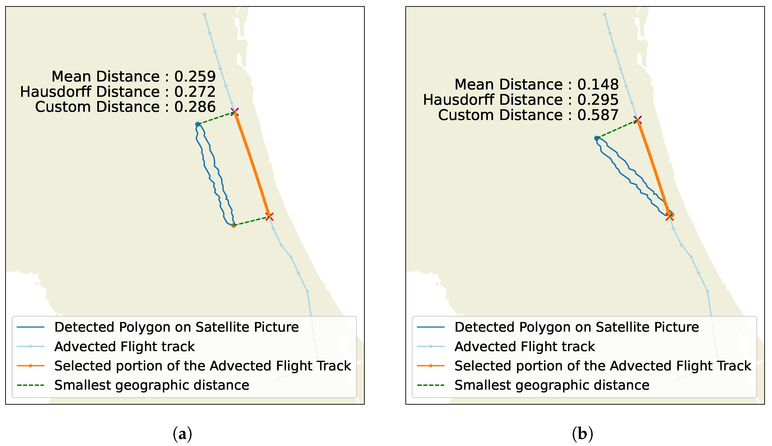
3.1. Single Frame Flights-Contrail Matching

This Section will explain the methodology employed to associate a polygon detected at a particular timestamp with the flights that could have generated it. As explained in the previous section, it is possible to estimate where each flight’s hypothetical contrail would be at time $t_i$, assuming the aircraft had produced a contrail at time $t_j$ with $t_j<t_i$. Figure 12 provides empirical insights on how the matching between the flight and the contrail polygon could be performed.

In order to define a first group of candidates, several filters were chosen. It was decided to only consider flights whose advected trace was within 1 degree of latitude and longitude from the polygon. The apparent heading difference between the polygon and the advected flight trace is used as a second filter. All advected traces with an angle of more than 7° with the polygon will not be considered as potential candidates either. A third filter was added based on the values of temperature at the location of the flight at the moment it potentially created a contrail. The maximum temperature for contrail formation is estimated to be −35 °C. It was decided to reject every trajectory in which the aircraft flew in an air mass at temperatures above −25 °C.

A more relevant filter using the Schmidt Appleman contrail formation criterion [30] was also considered, as it could provide a more relevant filter than that using a simple temperature threshold. However, in a significant number of cases this filtering ignored the flight that actually produced the contrail, probably because of uncertainties in the prediction of relative humidity forecast at these altitudes. In general, these cases were very close to the humidity and temperature thresholds required to satisfy the Schmidt-Appleman criterion, or very close to an area where this criterion was satisfied.

The result of this filtering process is a set of potential candidates, but this filtering alone is often not enough to find the aircraft responsible for the contrail.

It could be difficult to define a metric to measure the quality of the matching between an advected flight trace and a polygon. Given a specific flight and a specific polygon, several distances were defined.

Since no information is available on which portion of the flights produced the contrail, it was assumed that the portion of the advected flight path that is closest to the polygon is the most likely to have generated the contrail, as shown in Figure 13. It corresponds to the projection of the polygon on the advected flight track. This portion of the advected flight is used to build the metrics that will allow to discriminate between the candidates. It will be called the selected portion from now on.

Once the portion of the advected flight that has potentially produced the contrail could been identified this method is applied to select a set of probable candidates. Several metrics could then be used to discriminate between the candidates. They are computed between the selected portion and the centerline of the polygon, both re-sampled into 100 evenly separated points. The first metric used is a mean Haversine geographical distance between the contrail polygon points and the advected flight trace. It is formulated as follows:

$${\mathrm{d}}_{\mathrm{Mean}}(\mathrm{P},\mathrm{AFT})=\frac{1}{\left|\mathrm{P}\right|}\sum _{a\in \mathrm{P}}^{}\underset{b\in \mathrm{AFT}}{inf}\mathrm{d}(a,b)$$

(1)

where P is the list of the points corresponding to the centerline the polygon, $\left|\mathrm{P}\right|$ the number of points in the list P, and AFT the points in the corresponding selected portion of the advected flight trace. $\mathrm{d}(a,b)$ corresponds to the Harversine distance between two geographic points. This metric gives the averaged geographical distance between the two objects.

The main uncertainty about the position of the hypothetical contrail produced by the flight is the wind induced uncertainty. However, it seems that the uncertainty on wind speed is more pronounced than that of wind direction. Confidence is higher with a contrail that has the same heading and a bigger mean distance than a contrail that has a slightly lower mean distance but has a higher heading difference. In Figure 14, for example, we are more confident about the contrail/flight match in Figure 14a than we are with that in Figure 14b.

This is the reason why the Hausdorff distance was chosen as a second metric. It is defined as follows:

$${\mathrm{d}}_{\mathrm{H}}(\mathrm{P},\mathrm{AFT})=max\left\{\underset{a\in P}{sup}\underset{b\in AFT}{inf}\mathrm{d}(a,b),\underset{b\in AFT}{sup}\underset{a\in P}{inf}\mathrm{d}(a,b)\right\}$$

(2)

where P is the list of the points in the centerline of the polygon, and AFT the points in the corresponding selected portion of the advected flight trace.

This score also provides information about the distance between the polygon and the selected portion. However, by taking the sup value over the distances, this metric tends to give a greater weight to flights that have the same heading as the contrail, as shown in Figure 14.

Another metric could also be used, defined by:

$${\mathrm{d}}_{\mathrm{Custom}}(\mathrm{P},\mathrm{AFT})=\frac{{\mathrm{d}}_{\mathrm{H}}{(\mathrm{P},\mathrm{AFT})}^2}{{\mathrm{d}}_{\mathrm{Mean}}(\mathrm{P},\mathrm{AFT})}$$

(3)

This new metric gives a greater weight to the flights that are parallel to the polygon, even more than when using Hausdorff distance.

It is then possible to match the candidate polygons to the flights by optimization. The matching problem can be formulated as follows: let $a_{i,j}\in \{0,1\}$ be the binary decision variable, with i the index of the flight, j the index of the contrail polygon. $a_{i,j}=1$ when flight i matched with contrail j, and $a_{i,j}=0$ otherwise. Let $c_{i,j}$ be the flight-contrail correlation matrix defined by using the inverse of the flight-contrail distance described above.

$$\underset{\mathbf{a}}{\max } J(\mathbf{a},c)=\sum _{i,j}{a}_{i,j}{c}_{i,j}$$

(4a)

$$\mathrm{s}.\mathrm{t}. \sum _i{a}_{i,j}\le 1, j\in \mathrm{Contrail} \mathrm{Polygons}$$

(4b)

The constraint defined in (4b) expresses that each detected contrail could be matched with at most one flight.

However, it is often not enough to solve the matching problem, especially in areas with high flight density. Uncertainties in weather data such as wind have an important impact on the difference between the predicted and observed contrail position. The older the contrail, the greater the impact of these uncertainties. It has been measured that the candidate filter described above is susceptible to ignoring the actual aircraft at the source of the contrail when applied to a contrail older than one hour. Furthermore, the metrics based on the distance and orientation difference between the predicted and observed position of the contrail also lose relevance with increasing contrail age.

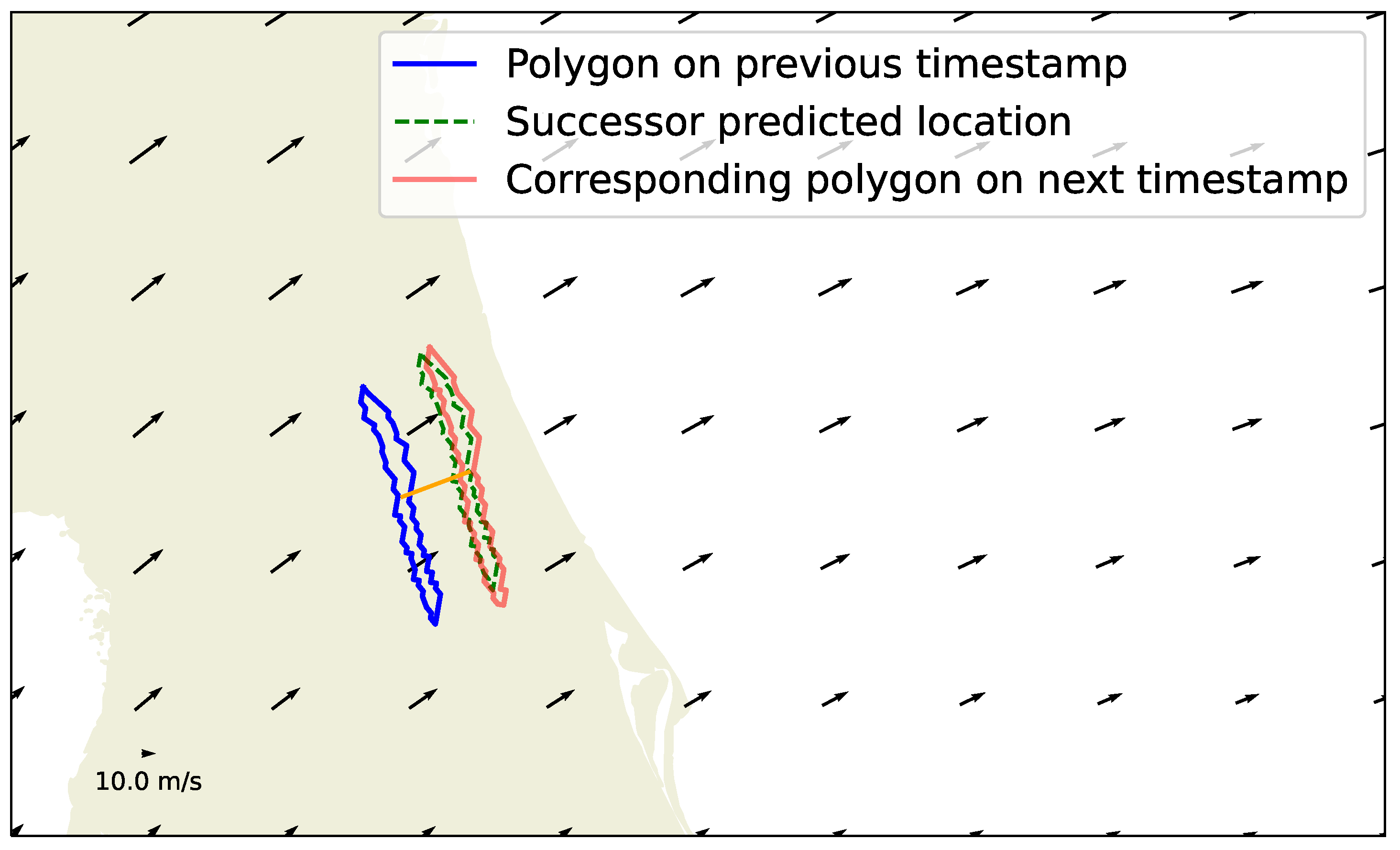
3.2. Tracking of Contrails Using Time Information

Even with all the different metrics previously defined, there are sometimes several flights that could still correspond to the polygons at a specific timestamp. In this section, temporal information is used to help discriminate between these flights. There is therefore a need for a contrail tracking method.

The lack of information about the altitude of the detected contrails makes it difficult to use the forecasted wind to find the successor of a polygon in the method developed in [12]. A workaround was found, but it requires a greater temporal resolution of the satellite sensors to overcome this problem. In this study, it was decided to use traffic data to formulate several guesses about the possible altitudes of the contrails, which would allow an estimate to be made of the wind conditions at that location. This information is used to find the potential successor of the polygon on the next picture, if it exists.

In order to guess the location of the polygon’s successor on the next frame, the same method as in the single frame flight-contrail matching from Section 3.1 is used to select the flights that have the highest probability to have caused the contrail. The altitude of these different flights are then used to estimate the wind conditions at the polygon’s location. This wind information allows to move the previous polygon into the several locations in which a potential successor could be expected.

If we note $[x_p\left(t\right),y_p\left(t\right)]$ the coordinates of the centroid of the polygon of the detected contrail on the Goes picture at time t, $z_C\left(t\right)$ the probable altitude of the contrail using the method described above, $[x_w(x_p,y_p,z_C,t),y_w(x_p,y_p,z_C,t)]$ the wind conditions at point ($x_p,y_p,z_C,t$), and $\mathsf{\Delta }t$ the difference between the timestamps of the two successive pictures, we have:

$$\{\begin{array}{c}\hfill x_p(t+\mathsf{\Delta }t)=x_p\left(t\right)+x_w(x_p,y_p,z_C,t)\mathsf{\Delta }t,\\ \hfill y_p(t+\mathsf{\Delta }t)=y_p\left(t\right)+y_w(x_p,y_p,z_C,t)\mathsf{\Delta }t,\end{array}$$

(5)

The polygons that overlap with this advected polygon and that have a small difference in heading could be considered to be the successors. For example, in Figure 15, a polygon from the next frame matches with the polygon selected on the previous frame.

This advection process is applied using the mean altitudes of all the candidate altitudes as described above. Most of the time, the only potential successors are found using the most probable candidate’s wind values. However, in very crowded areas, other successors can be found at different altitudes, with other wind conditions. It is at this point difficult to decide which ones are actually the right successors, but this method still brings valuable information.

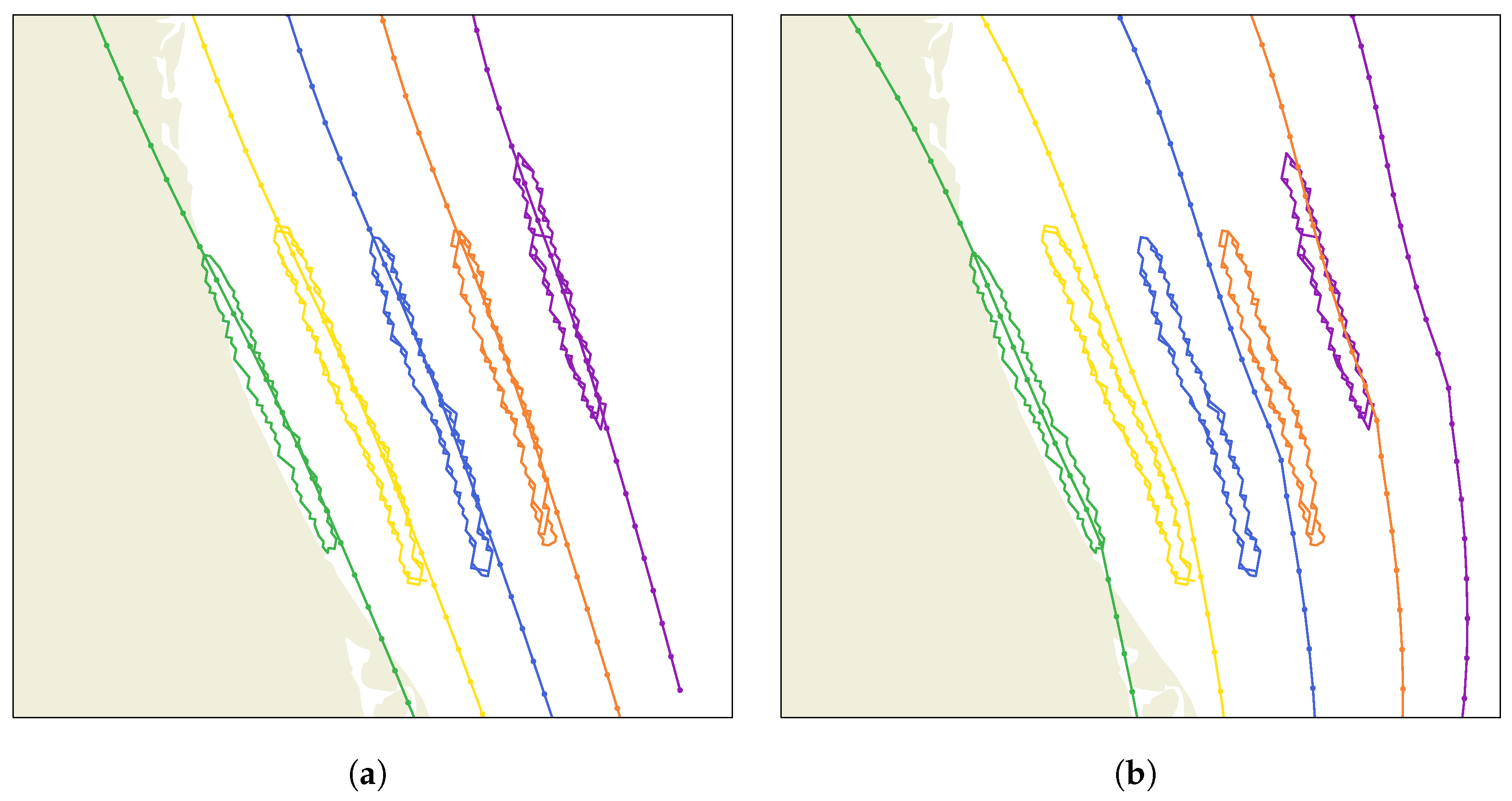
3.3. Combining Both Approaches

Two methods were described in the previous section. The first one allows us to select the flights that could have produced a contrail detected on a satellite image. It is however not always able to discriminate between these flights especially in crowded areas. The second method attempts to identify the polygons that correspond to the same contrail on the next satellite picture, but it is subject to wind uncertainties and may select two incompatible successors for the same detected contrail. However, combining information from both methods can help us accurately discriminate between all candidates.

It is possible to use the method described in Section 3.1 to select a given polygon’s “flight candidates”, a small set of flights that could have caused the contrail formation. This filtering process removes the flights that are not close enough, have an advected flight trace with too much difference in angle with the polygon, or are not flying in a cold enough area to have produced a contrail.

Based on the procedure from Section 3.2, Algorithm 1 is used to sample the most probable chain of polygons given the first polygon of the chain and a flight candidate.

Each polygon detected on the satellite images could potentially be the first time a contrail is seen, so it is possible to iterate on the detected polygons and on their candidates to generates all the most probable chains starting with each polygon.

Algorithm 2 iterates through all the detected polygons and their respective flight candidates, and uses Algorithm 1 to generate and evaluate all the most probable chains of polygons from these.

Algorithm 1 Generation of a chain of polygons from a candidate flight and a first polygon.

procedure Build_Chain($Polygon,Flight$) ▹$Polygon$ is the first polygon of the chain, $Flight$ is the flight selected to build the chain     $Chain\leftarrow \left\{Polygon\right\}$     $Successor\leftarrow Polygon$     $CurrentPolygon\leftarrow Polygon$     while $Successor\mathrm{is}\mathrm{not}\mathrm{NULL}$ do         $T\leftarrow \mathrm{time}\mathrm{at}\mathrm{which}CurrentPolygon\mathrm{was}\mathrm{detected}$         $Weather\leftarrow \mathrm{GET}\_\mathrm{WEATHER}(Polygon,Flight,T)$ ▹ This function gets weather data at location of $CurrentPolygon$, at time T, with the altitude information from $Flight$.         $Successor\leftarrow \mathrm{GET}\_\mathrm{SUCCESSOR}(CurrentPolygon,Weather,T)$ ▹ This function checks if a potential successor is present on the next frame like shown in Figure 15         $Chain\leftarrow Chain+Successor$         $CurrentPolygon\leftarrow Successor$     end while     return $Chain,Flight$ end procedure

Algorithm 2 Generation and Evaluation the list of possible contrails chains.

$PolygonsList\leftarrow \mathrm{List}\mathrm{of}\mathrm{all}\mathrm{detected}\mathrm{Polygons}$ $ChainScores\leftarrow \left\{\right\}$ for $Polygon\in PolygonsList$ do     $CandidatesList\leftarrow \mathrm{GET}\_\mathrm{CANDIDATES}\left(Polygon\right)$     for $Candidate\in CandidatesList$ do         $Chain\leftarrow \mathrm{BUILD}\_\mathrm{CHAIN}(Polygon,Candidate)$         $Score\leftarrow \mathrm{EVALUATE}\_\mathrm{CHAIN}(Chain,Candidate)$         $ChainScores\leftarrow ChainScores+(Chain,Score)$     end for end for

This method pre-computes a set of “potential chains”, each characterised by a flight, and a set of polygons, in which will be included the chains representing the true contrails. It is possible to reformulate the tracking and matching problem into: which of the generated chains are true contrails?

To reduce the amount of unnecessary candidates, it is possible to remove all the chains that could not realistically be contrails. First, the same filtering as presented in Section 3.1 is used.

Each chain is supposed to represent a whole contrail. This allows for a new type of filtering, taking for example into account the time between the aircraft passage and the first detection of the contrail. The resolution of Goes images is a few kilometers squared, which means that young contrails may not be immediately visible on these images. It can take anywhere from a few minutes to half an hour for the contrails to become visible on Goes images. This information can help us filter out the less probable candidates by disregarding the flights that passed after the first contrail was detected (obviously not a good candidate) or those that passed too early before it was detected, as it is doubtful the contrail stayed undetected for such a long period of time. It was decided to ignore the chains for which the time between the plane passage and the first observation of the contrail is more than forty minutes or less than one minute.

Other filters could also be added. The first polygon of the chains represents the first time the contrail is ever observed. The matching between the polygons and the flights is subject to wind uncertainties. These uncertainties have an impact on the location of the advected flight trace that needs to be matched with the detected contrail. As the flight trace is advected for a longer period of time, the uncertainties on its position gets higher. The matching with an advected flight trace of the first polygon is therefore subject to less wind uncertainty. It was decided to set a threshold on the minimum score that the polygon/flight matching should perform for the first polygon to ensure the quality of the matching of the beginning of the chain.

Then, having filtered out as many unrealistic chains as possible, it is possible to formulate a new matching problem.

Let $a_{i,j}\in \{0,1\}$ be the binary decision variable, with i the index of the flight, j the index of the chain of polygon. $a_{i,j}=1$ when flight i is matched with chain j, and $a_{i,j}=0$ otherwise.

Let $b_{j,k}\in \{0,1\}$ be the chain-polygon correspondence matrix. This matrix is built beforehand, using the list of all the potential polygon chains. $b_{j,k}=1$ when chain j contains polygon k, and $b_{j,k}=0$ otherwise.

Let $c_{i,k}$ be the flight-contrail correlation matrix defined by using the inverse of the flight-contrail distance described above.

Let $d_{i,j}$ be the flight-chain matrix describing the delta of time between the passage of the aircraft and the first observation of the contrail.

The optimization problem maximizing the score of the matching while choosing between incompatible options could be formulated as follow:

$$\underset{\mathbf{a}}{\max } J(\mathbf{a},b,c)=\sum _{i,j}{a}_{i,j}\sum _k{b}_{j,k}{c}_{i,k}$$

(6a)

$$\mathrm{s}.\mathrm{t}. \sum _{i,j}{a}_{i,j}{b}_{j,k}\le 1, k\in \mathrm{Contrails},$$

(6b)

$$\sum _i{a}_{i,j}{d}_{i,j}\le 40\min , j\in \mathrm{Chains},$$

(6c)

$$\sum _i{a}_{i,j}{d}_{i,j}\ge 1\min , j\in \mathrm{Chains}$$

(6d)

The first constraint (Equation (6b)) assures that each contrail could only be assigned to one flight. This is a rather strong assumption because some contrails might sometimes overlap, but it allows the problem to be modeled using an optimization approach.

The second and third constraints (Equations (6c) and (6d)) correspond to the verification that the time between the flight passage and the contrail first detection makes sense: a contrail that will appear on the satellite picture more than 40 min after the passage of the aircraft will not be matched with this flight, whatever the score.

By formulating the problem in this way, it is reduced into a MILP (mixed-integer linear program) type problem. The result of this optimization process is composed of the indices of the flight/chains that were selected.

The generation of the polygon chains enumerates the possible contrails in an exhaustive way. It means that the final set of possible chains contains numerous incompatible options. The optimization based method allows one to choose between these incompatible candidates like shown in Figure 16.

The following paragraph illustrates how the method operates, starting with a reminder of some of the terms defined earlier.

A frame (as a picture from a video) is a satellite image taken at a specific time. A polygon represents the boundaries of a contrail on a frame, thus at a specific time. It is the output of the detection method. An advected flight trace represents the predicted position of the contrail produced by a flight at a given time, assuming that contrails are formed along the entire trajectory. A chain of polygons is a sequence of polygons describing the positions of a potential contrail on successive frames. A chain is defined by a first polygon, a flight, and the list of the polygons that describe the position of the contrail on the following frames. These chains are built using the Algorithms 1 and 2. A set of selected chains is chosen by optimization. The optimization process performs choices between the incompatible chains.

On 1 January 2019, at 13:20 UTC, just next to a cluster of contrails, two contrails were detected in a region in which several aircraft flew a few minutes before. The detection method detected several objects on the following frames. The situation is described in Figure 17.

As shown in Algorithm 2, the chain generation process is applied to each detected polygon. Given a polygon P, a chain is defined for each flight which advected flight trace passed the filter described in Section 3.1. These flights are what we called the candidates. For each pair (P, candidate), a chain will be defined by finding all the successors of the polygon P according to the method described in Section 3.2 given the wind conditions derived from the information provided by the flight candidate. The result of this iterative process is a set of chains of polygons, each defined by the flight and the first polygon used to define it. Given the situation presented in Figure 17, six chains were generated. They are presented in Figure 18.

Several chains in the set could be incompatible with respect to the chosen constraints. In this case, chain 1 (Figure 18a) is incompatible with chain 5 (Figure 18e), because several polygons are shared between the two chains, and a single polygon cannot be attributed to a single flight. The score of chain 5 is higher, so we remove chain 1 from the set.

Chain 3’s (Figure 18c) polygons are shared with chain 2 (Figure 18b), and they belong to the same flight. It could happen when the second polygon corresponding to the contrail is detected less than 40 min after the contrail formation. In order to not count the same polygons twice, and because chain 2 also covers more polygons, chain 3 is removed from the set. The same situation is applied to chains 5 (Figure 18e) and 6 (Figure 18f). Chain 6 is therefore removed from the set.

Chain 2’s (Figure 18b) polygons are shared with chain 4 (Figure 18d), and they belong to different flights. Flight DAL2027 passed in the area after flight RPA4727, so it couldn’t capture the first polygon of the chain captured by flight RPA4727, and the score of its chain is also lower. Chain 2 is therefore removed from the set.

This process lead to the selection of the two chains presented here in Figure 19.

The main advantage of a method solving the matching and tracking of all contrails at the same time is that it can use information from the context around the contrail (tracking three parallel contrails matched with three parallel flights is easier than tracking each of them separately). Just as the human operator would, the optimization method will maximize the overall score of the matching, even when wind uncertainty makes the position of the real contrails slightly different from the predicted ones.

4. Case Study

4.1. Results on Contrail Tracking

The method has been applied for example purpose on a 8 h period the 1 January 2019, from 12:00 UTC to 21:00 UTC, over an area covering the continental US (latitude between 20 N and 60 N, and longitude between 125 W and 40 W). A lot of contrails can be observed during this period. It includes several interesting situations: we have both isolated distinct contrails, and overlapping contrails in crowded areas. It could therefore be interesting to describe a few situations encountered.

This case study illustrates the potential of this kind of method in order to build a dataset of observational data that could be used to help validate the contrail models. It also shows in which aspect the method could still be improved.

4.1.1. Description of the Case Study

In this 8 h period, 26,394 polygons were detected on the satellite images (note that a particular contrails can be detected several times in our detection method). There are 8989 distinct flights in the ADSB traffic data over this period in the area. Using the method described above, and after filtering, Algorithm 2 allowed us to precompute a total of 16,087 distinct chains and to evaluate each one of them.

The optimization process resulted in 3680 chains being selected, with a total of 1552 flights producing contrails at some point during the flight.

The time between the flight passage and the first observation of the contrail is 27 min on average over the test case. Note that because the time between two frames is 15 min, this value does not correspond to the time it really takes for a contrail to potentially become visible on a geostationary satellite image. For example, the use of the Mesoscale product of Goes 16 (with a time resolution of one minute) should show a different (probably much shorter) value. This value also heavily depends on the detection method used, and its ability to detect thin young contrails, not yet very distinct from the background.

Contrail observed persistence time distribution is described in Figure 20. The contrail tracked for the longer period of time lasted about 4 h in our test case. It is shown in Figure 21.

This contrail was detected on 14 different frames. However, it was already visible on the frame before the first detection by the algorithm. It is also still visible on the frame after the last detection by the algorithm, even if at this point it has lost its linear shape. It is also interesting to note that the detection algorithm only highlighted the part of the contrail showing a higher contrast with the background.

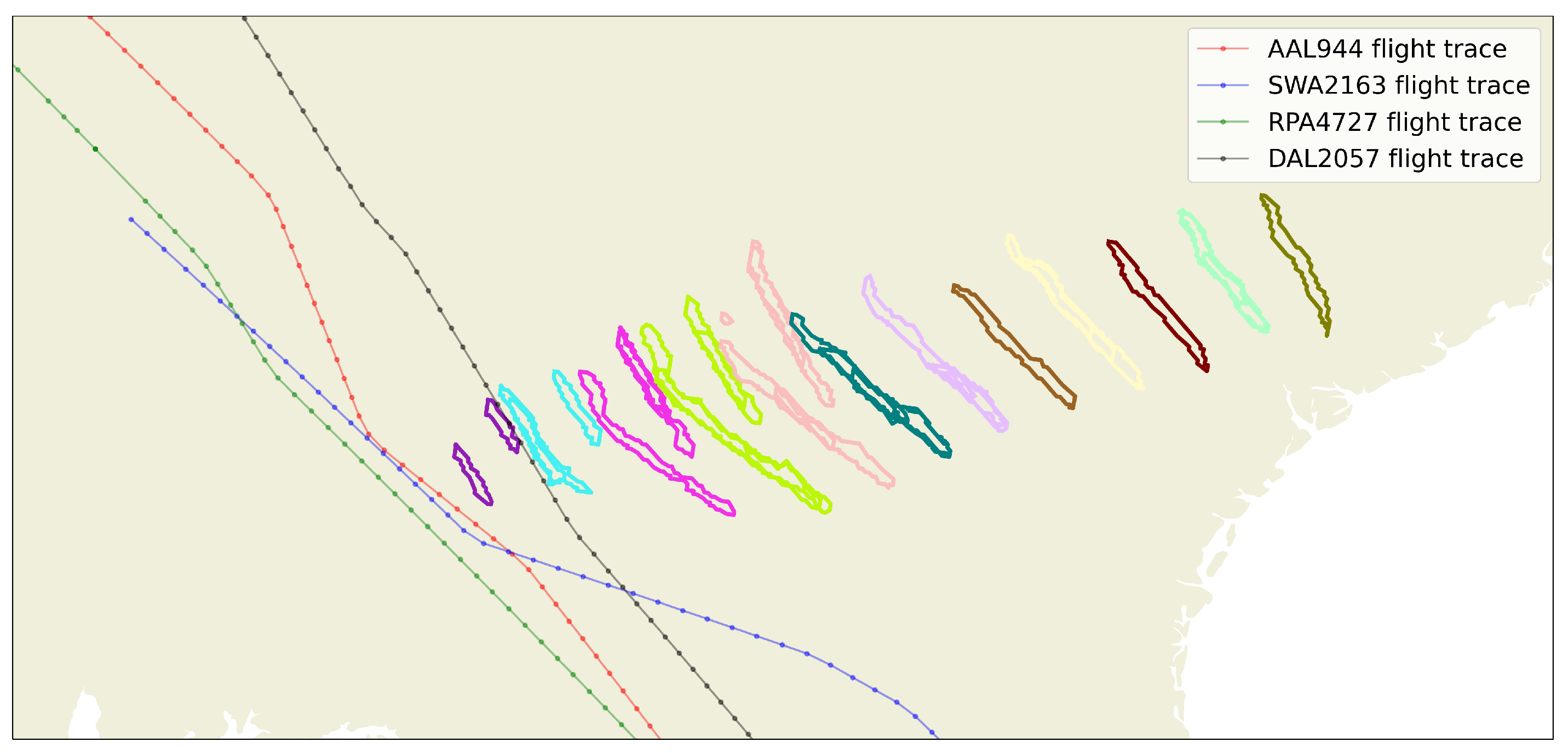
4.1.2. Isolated Contrails: High Confidence on a Small Set of Examples

Sometimes, isolated aircrafts can cross contrail formation areas. These are often the most easy contrails to identify and track as there is only one candidate for the identification of the contrail, and knowing for sure which flight is responsible for creating a contrail makes the tracking problem much easier to solve, even for long-lasting contrails.

For every chain of polygons that were generated, we consider that it represents an isolated contrail if the first polygon of the chain has only one valid candidate according to the various filters described in Section 3.3. It means that the corresponding advected flight trace must be close enough to this polygon at the time it was detected, that the aircraft originally flew in an area in which the temperature was compatible with contrail formation, and that the time between the passage of the aircraft and the detection of the contrail is between 1 min and 40 min.

There were several occurrences of these isolated long-lasting contrails in our test case. For example, over this period of time, 26 isolated contrails, lasting more than 1 h and detected on at least three successive frames were reported.

These cases are interesting as they provide valuable information about to what extent the advected flight track is actually close to the corresponding contrail. It also indicates how this difference evolves overtime, thus giving information about the expected quality of our matching and tracking method.

They could also be used to test the validity of contrail prediction methods.

4.1.3. Contrails Forming in an Empty Area

Some contrails form in a region in which there were no contrails detected on the previous frames. There is a high probability that such a chain describes a real contrail, and not a subset of an older contrail. Confidence on tracking is therefore higher in this case than for the contrails forming in crowded areas.

There are 659 contrails detected on at least two frames in this experiment. 535 of them formed in an empty region, with no polygons in the area on the timestamp before their formation, while 124 formed in regions where polygons had already been detected. In order to define these regions, it is possible to select all the different flight candidates matching this chain of polygon, and use the subsequent wind information to look back in time if there was any detected contrails matching the predicted positions of a potential previous polygon.

4.1.4. Performance on Difficult Situations

Even for contrails with several potential candidates with no guarantee about the quality of the result, it is often possible to qualitatively check the validity of the selected chains of polygons.

The main advantage of combining wind and traffic data in this method is the ability to distinguish between close parallel contrails from aircraft flying close to one another. If the two aircraft produce a contrail, it is possible to choose which chain of polygons is from which flight, as shown in Figure 22.

A tracker without wind information could misidentify the successor of a polygon, leading to incorrect results. A tracking method that does not take into account the fact that a contrail can only have been issued by one aircraft would also risk associating the same contrail with several aircraft, or incorrectly associating a contrail to an aircraft that did not produce any.

The interest of our method in this context is to restrict the successor search to avoid selecting a polygon belonging to another contrail to continue tracking. It therefore allows parallel contrails to be correctly identified and tracked.

In this example, there are only two aircraft with a high enough score to have produced the contrails. Their positions relative to the proposed chains makes it easy for a human to check which contrail was produced by which flight. In this case, it is therefore possible to assess whether the method proved successful.

4.2. Limitations

This method allows to extract valuable information from the traffic data and the satellite images, but some limitations have to be highlighted.

4.2.1. Detection Based Tracking Algorithm

This method is a detection based tracker. To be able to correctly track an object through the successive frames, it is important that the object is detected on all of these frames. The consistency of the detection method is therefore of great importance for the quality of the overall result. In our case, it is not uncommon to lose track of a contrail because it was missed by the detector after a few frames.

The detection method is also trained to detect only linear contrails. It can sometimes continue to detect them when they lose their linear shape, but cannot detect them when their appearance becomes too similar to natural cirrus. It is also difficult to detect sub-pixel wide contrails and contrails with low optical depth, which reduces the contrast with the background, especially in areas with natural cirrus and other contrails.

4.2.2. Lack of Confidence for Short Lived Contrails

The method presented in this study relies among others on contrail’s observed wind advection to discriminate between potential candidates. In this context, the longer the contrail persists, the greater the confidence will be. In fact, the drift due to differences between predicted and observed wind will become more visible with a longer persistence time. Therefore, when the contrail has a short lifetime (visible on only one or two frames), the use of observed advection provides less information, thus leading to a higher risk of contrail misidentification (matching with the wrong flight).

Observation of the contrail evolution also allows to remove most detection false positives. It means that if the model detected a feature on the satellite image that is not a contrail, there is only a small risk that an aircraft advected flight trace matches perfectly with this false contrail on several timestamps. However, it is possible that it matches on only one frame. This is why a contrail lasting only one frame in our results has a higher risk to actually be a false positive from the detector.

In the test case chosen here, 1690 contrails visible on only one frame were identified. Over these 1690 contrails, 493 formed at a place and time where only one flight could match them with a sufficient score.

4.2.3. Wind Uncertainties over Large Periods of Time

When studying a contrail lasting several hours, it is not uncommon to witness a “drift” between the predicted and the observed contrail’s locations. This is not a problem to study the beginning of the contrail lifetime, but after a few hours, the contrail might have drifted too far away from the predicted location. Another flight could then happen to match the contrail better the contrail at this point, leading to misidentification.

This would mean that the method will lose track of the original contrail, and attribute a contrail to the second aircraft, even if it might not have produced one. To solve this problem, a factor could be applied to the longer lasting contrails to give them a greater weight against this kind of issue. However, a dataset of ground truth contrail tracking and matching would be needed in order to correctly set these parameters.

4.2.4. Lack of Validation Data

The only other contrail tracking method published to this day is ACTA [12], which is applied to Europe. No dataset about contrail identification and tracking was published either. We were therefore unable to access data that could be used to further validate our model. It is however likely that improvement could be made confronting the model with ground truth data. An example of a possible way to improve this method was discussed in the previous paragraph. It could also be interesting to get more quantitative information on the performance and robustness of our method.

5. Conclusions and Future Work

5.1. Conclusions

This study presents a novel approach to monitor contrails throughout their evolution and to identify the aircraft responsible for their formation. This method leverages air traffic data, weather data as well as geostationary satellite images to achieve this task. It improves the reliability of the tracking and the flight identification problems by solving them together.

The aim of this study is not to allow an exhaustive monitoring of all the contrails at a given time, but to allow the identification of a set of contrails for which the tracking and the flight matching can be done with a given confidence. Such a dataset could then be combined with data from ground cameras, other types of satellites, or sensors to create a dataset of identified contrails that provides information on the different phases of contrail evolution. Although much of the climate impact of contrails is caused by cirrus contrails that have already lost their linear shape, we believe it is interesting to use the period when they still have it to identify the aircraft that caused them and to provide useful information for initiating the tracking of the contrail in its spread form. This study will therefore be important in order to join several observation methods, each characterising different aspects of the contrails. Ultimately, this will allow progress to be made in the validation of climate impact models of contrails.

To be able to build a dataset in order to help validate contrail climate impact models, there is a need for information on the formation of the contrail, on its evolution, and on its physical properties all along its persistence time. This study proposes a way to gather information about the evolution of the contrail, but it will need to be supplemented by other data sources to gather information on the other aspects. However, the use of this method allows to easily merge the dataset with other means of observation, as the aircraft that produced the contrail is well identified.

5.2. Future Work

The limitations of our method described in Section 4.2 point to potential future work extending this study. In order to conduct more global studies, contrail detection on satellite images still needs to be improved. The consistency of the detection in particular needs improving. It will also be interesting to use more global air traffic data, including for example satellite based ADSB data improving the results over the oceans.

In order to further improve the results of the method, there is a need for a ground truth dataset to help adjust the different parameters and metrics used here.

It is already possible to use the information generated by our method to validate several aspects of the contrail simulation models. However, in order to be able to validate the climate impact modeling, this method needs to be coupled with a radiative forcing estimation method. It will also be necessary to be able to track the contrails beyond the period in which they maintain their linear shape. We believe that our method provides a good way to initialize such a tool by identifying the flight causing the contrail and tracking the first positions of the linear contrail.

References

1. Lee, D.S.; Fahey, D.W.; Skowron, A.; Allen, M.R.; Burkhardt, U.; Chen, Q.; Doherty, S.J.; Freeman, S.; Forster, P.M.; Fuglestvedt, J.; et al. The contribution of global aviation to anthropogenic climate forcing for 2000 to 2018. Atmos. Environ. 2021, 244, 117834. [Google Scholar] [CrossRef] [PubMed]
2. Schumann, U. A contrail cirrus prediction model. Geosci. Model Dev. 2012, 5, 543–580. [Google Scholar] [CrossRef] [Green Version]
3. Burkhardt, U.; Kärcher, B. Global radiative forcing from contrail cirrus. Nat. Clim. Chang. 2011, 1, 54–58. [Google Scholar] [CrossRef] [Green Version]
4. Chen, C.C.; Gettelman, A. Simulated radiative forcing from contrails and contrail cirrus. Atmos. Chem. Phys. 2013, 13, 12525–12536. [Google Scholar] [CrossRef] [Green Version]
5. Frömming, C.; Volker, G.; Jockel, P.; Brinkop, S.; Dietmüller, S.; Garny, H.; Ponater, M.; Tsati, E.; Matthes, S. Climate cost functions as a basis for climate optimized flight trajectories. In Proceedings of the 10th USA/Europe Air Traffic Management Research and Development Seminar, ATM 2013, Chicago, IL, USA, 10–13 June 2013. [Google Scholar] [CrossRef]
6. Yin, F.; Grewe, V.; Castino, F.; Rao, P.; Matthes, S.; Dahlmann, K.; Dietmüller, S.; Frömming, C.; Yamashita, H.; Peter, P.; et al. Predicting the climate impact of aviation for en-route emissions: The algorithmic climate change function submodel ACCF 1.0 of EMAC 2.53. Geosci. Model Dev. Discuss. 2023, 16, 3313–3334. [Google Scholar] [CrossRef]
7. Mannstein, H.; Meyer, R.; Wendling, P. Operational detection of contrails from NOAA-AVHRR-data. Int. J. Remote. Sens. 1999, 20, 1641–1660. [Google Scholar] [CrossRef]
8. Kulik, L. Satellite-Based Detection of Contrails Using Deep Learning. Master’s Thesis, Massachusetts Institute of Technology, Department of Aeronautics and Astronautics, Cambridge, MA, USA, 2019. [Google Scholar]
9. Knapp, K.R.; Wilkins, S.L. Gridded satellite (GridSat) GOES and CONUS data. Earth Syst. Sci. Data 2018, 10, 1417–1425. [Google Scholar] [CrossRef] [Green Version]
10. Ronneberger, O.; Fischer, P.; Brox, T. U-net: Convolutional networks for biomedical image segmentation. In Medical Image Computing and Computer-Assisted Intervention–MICCAI 2015: 18th International Conference, Munich, Germany, 5–9 October 2015, Proceedings, Part III 18; Springer: Berlin/Heidelberg, Germany, 2015; pp. 234–241. [Google Scholar] [CrossRef] [Green Version]
11. Meijer, V.R.; Kulik, L.; Eastham, S.D.; Allroggen, F.; Speth, R.L.; Karaman, S.; Barrett, S.R. Contrail coverage over the United States before and during the COVID-19 pandemic. Environ. Res. Lett. 2022, 17, 034039. [Google Scholar] [CrossRef]
12. Vazquez-Navarro, M.; Mannstein, H.; Mayer, B. An automatic contrail tracking algorithm. Atmos. Meas. Tech. 2010, 3, 1089–1101. [Google Scholar] [CrossRef] [Green Version]
13. Simorgh, A.; Soler, M.; González-Arribas, D.; Matthes, S.; Grewe, V.; Dietmüller, S.; Baumann, S.; Yamashita, H.; Yin, F.; Castino, F.; et al. A Comprehensive Survey on Climate Optimal Aircraft Trajectory Planning. Aerospace 2022, 9, 146. [Google Scholar] [CrossRef]
14. Gierens, K.; Matthes, S.; Rohs, S. How well can persistent contrails be predicted? Aerospace 2020, 7, 169. [Google Scholar] [CrossRef]
15. Agarwal, A.; Meijer, V.R.; Eastham, S.D.; Speth, R.L.; Barrett, S.R. Reanalysis-driven simulations may overestimate persistent contrail formation by 100%–250%. Environ. Res. Lett. 2022, 17, 014045. [Google Scholar] [CrossRef]
16. Wang, Z.; Bugliaro, L.; Jurkat-Witschas, T.; Heller, R.; Burkhardt, U.; Ziereis, H.; Dekoutsidis, G.; Wirth, M.; Groß, S.; Kirschler, S.; et al. Observations of microphysical properties and radiative effects of a contrail cirrus outbreak over the North Atlantic. Atmos. Chem. Phys. 2023, 23, 1941–1961. [Google Scholar] [CrossRef]
17. Schmit, T.J.; Griffith, P.; Gunshor, M.M.; Daniels, J.M.; Goodman, S.J.; Lebair, W.J. A Closer Look at the ABI on the GOES-R Series. Bull. Am. Meteorol. Soc. 2017, 98, 681–698. [Google Scholar] [CrossRef]
18. Schäfer, M.; Strohmeier, M.; Lenders, V.; Martinovic, I.; Wilhelm, M. Bringing up OpenSky: A large-scale ADS-B sensor network for research. In Proceedings of the IPSN-14 Proceedings of the 13th International Symposium on Information Processing in Sensor Networks, Berlin, Germany, 15–17 April 2014; pp. 83–94. [Google Scholar] [CrossRef]
19. Hersbach, H.; Bell, B.; Berrisford, P.; Biavati, G.; Horányi, A.; Sabater, J.M.; Nicolas, J.; Peubey, C.; Radu, R.; Rozum, I.; et al. ERA5 Hourly Data on Pressure Levels from 1959 to Present. Copernicus Climate Change Service (C3S) Climate Data Store (CDS), 2018. Available online: https://doi.org/10.24381/cds.adbb2d47 (accessed on 10 April 2023).
20. Teoh, R.; Schumann, U.; Gryspeerdt, E.; Shapiro, M.; Molloy, J.; Koudis, G.; Voigt, C.; Stettler, M.E.J. Aviation contrail climate effects in the North Atlantic from 2016 to 2021. Atmos. Chem. Phys. 2022, 22, 10919–10935. [Google Scholar] [CrossRef]
21. Boulanger, D.; Bundke, U.; Gallagher, M.; Gerbig, C.; Hermann, M.; Nédélec, P.; Rohs, S.; Sauvage, B.; Ziereis, H.; Thouret, V.; et al. IAGOS Final Quality Controlled Observational Data L2—Time series, Aeris [Data Set], 2018. Available online: https://doi.org/10.25326/06 (accessed on 10 April 2023).
22. McCloskey, K.; Geraedts, S.; Jackman, B. A Human-Labeled Landsat-8 Contrails Dataset. Tackling Climate Change with Machine Learning Workshop at ICML 2021. 2021. Available online: https://www.climatechange.ai/papers/icml2021/2 (accessed on 10 April 2023).
23. Sun, J.; Hoekstra, J.M.; Ellerbroek, J. OpenAP: An open-source aircraft performance model for air transportation studies and simulations. Aerospace 2020, 7, 104. [Google Scholar] [CrossRef]
24. He, K.; Gkioxari, G.; Dollár, P.; Girshick, R. Mask r-cnn. In Proceedings of the IEEE International Conference on Computer Vision, Venice, Italy, 22–29 October 2017; pp. 2961–2969. [Google Scholar] [CrossRef]
25. Ren, S.; He, K.; Girshick, R.; Sun, J. Faster r-cnn: Towards real-time object detection with region proposal networks. Adv. Neural Inf. Process. Syst. 2015, 28, 1137–1149. [Google Scholar] [CrossRef] [PubMed] [Green Version]
26. Lin, T.Y.; Maire, M.; Belongie, S.; Hays, J.; Perona, P.; Ramanan, D.; Dollár, P.; Zitnick, C.L. Microsoft coco: Common objects in context. In Computer Vision–ECCV 2014: 13th European Conference, Zurich, Switzerland, 6–12 September 2014, Proceedings, Part V 13; Springer: Berlin/Heidelberg, Germany, 2014; pp. 740–755. [Google Scholar] [CrossRef] [Green Version]
27. Girshick, R.; Donahue, J.; Darrell, T.; Malik, J. Rich feature hierarchies for accurate object detection and semantic segmentation. In Proceedings of the IEEE Conference on Computer Vision and Pattern Recognition, Columbus, OH, USA, 23–28 June 2014; pp. 580–587. [Google Scholar] [CrossRef] [Green Version]
28. Xie, S.; Girshick, R.; Dollar, P.; Tu, Z.; He, K. Aggregated Residual Transformations for Deep Neural Networks. In Proceedings of the IEEE Conference on Computer Vision and Pattern Recognition (CVPR), Honolulu, HI, USA, 21–26 July 2017; pp. 1492–1500. [Google Scholar] [CrossRef] [Green Version]
29. Lin, T.Y.; Dollár, P.; Girshick, R.; He, K.; Hariharan, B.; Belongie, S. Feature Pyramid Networks for Object Detection. In Proceedings of the 2017 IEEE Conference on Computer Vision and Pattern Recognition (CVPR), Honolulu, HI, USA, 21–26 July 2017; pp. 936–944. [Google Scholar] [CrossRef] [Green Version]
30. Schumann, U. On conditions for contrail formation from aircraft exhausts. Meteorol. Z. 1996, 5, 4–23. [Google Scholar] [CrossRef]
Figure 1. The Methodology developed in this study.
Aerospace 10 00578 g001
Figure 2. Reprojection of the satellite images: Orthographic projection centered on continental US allowing to minimize distortion. (a) Geostationary image centered on the US, corresponding to Goes CONUS product. (b) Reprojected image: the orthographic projection minimizing distortion over the US.
Aerospace 10 00578 g002
Figure 3. The principle of the method proposed by Appendix A12 of Schumann [2]. It allows to compute the contribution of each pixel to the optical depth of the simulated contrail according to the distance between the center of the pixel and the contrail central axis.
Aerospace 10 00578 g003
Figure 4. Description of the method used to study the difference in color between the contrail and the background.
Aerospace 10 00578 g004
Figure 5. Comparison of the distributions of the color change induced by the contrail per channel (red, green blue) between the hand labelled contrails and our synthetic contrail generation method.
Aerospace 10 00578 g005
Figure 6. Description of the method used to turn a simulated contrail mask into a synthetic contrail.
Aerospace 10 00578 g006
Figure 7. CoCiP simulated contrails turned into a realistic synthetic satellite image. (a) Simulated contrails from CoCip turned into a set of polygons. (b) Polygons added in a GOES tile free of real contrails.
Aerospace 10 00578 g007
Figure 8. The bounding boxes are overlapping: if not tuned correctly, non maximum suppression might delete the object with the lowest confidence score even if two different contrails were actually detected in the first place.
Aerospace 10 00578 g008
Figure 9. This image contains linear shapes that look like condensation trails but are not.
Aerospace 10 00578 g009
Figure 10. Result of contrail detection on real contrails. (a) Example of an unmodified GOES tile. (b) Detected contrails on this tile.
Aerospace 10 00578 g010
Figure 11. Advection of the Flight Track with the wind. These lines correspond to the position at which a potential contrail would be located at the indicated time.
Aerospace 10 00578 g011
Figure 12. Checking the quality of the matching between a detected contrail and two different flight tracks: advected flight track at timestep 6 needs to match the position of the polygon detected at timestamp 6. (a) Simulated contrail position matches the position of the contrail detected at timestamp 6. (b) Simulated contrail position doesn’t match the position of the contrail detected at timestamp 6.
Aerospace 10 00578 g012
Figure 13. Selection of the portion of the flight that most probably produced the contrail.
Aerospace 10 00578 g013
Figure 14. Contrail in the first situation must have a better score than in the second situation. (a) Contrail parallel to the track. (b) Contrail not parallel to the track.
Aerospace 10 00578 g014
Figure 15. Selection of the successors of the detected contrail on the next frame.
Aerospace 10 00578 g015
Figure 16. Examples of matching including tracking: the flight on the left picture gives a better match for the first polygon of the chain (on the left), but the evolution of the advected flight track does not match the evolution of the tracked contrail. (a) The contrail matches the advected flight track over the whole experiment. (b) The contrail drifts away from the advected flight track even if the first match is better.
Aerospace 10 00578 g016
Figure 17. The situation at the beginning of the illustration example. Several polygons are detected on successive frames, and four flights flew in the area moments before the first polygons were detected.
Aerospace 10 00578 g017
Figure 18. Chains generated from the situation presented in Figure 17. (a) Chain 1 from flight AAL944 and polygon 2790. (b) Chain 2 from flight DAL2057 and polygon 3106. (c) Chain 3 from flight DAL2057 and polygon 3627. (d) Chain 4 from flight RPA4727 and polygon 2824. (e) Chain 5 from flight SWA2163 and polygon 2790. (f) Chain 6 from flight SWA2163 and polygon 3118.
Aerospace 10 00578 g018
Figure 19. Final set of selected chains after the optimization process.
Aerospace 10 00578 g019
Figure 20. Distribution of the time of persistence of the tracked contrails.
Aerospace 10 00578 g020
Figure 21. A long lasting contrail in the test case.
Aerospace 10 00578 g021
Figure 22. Matching and tracking two contrails close and almost parallel: difficult without wind and traffic data.
Aerospace 10 00578 g022
Disclaimer/Publisher’s Note: The statements, opinions and data contained in all publications are solely those of the individual author(s) and contributor(s) and not of MDPI and/or the editor(s). MDPI and/or the editor(s) disclaim responsibility for any injury to people or property resulting from any ideas, methods, instructions or products referred to in the content.