Cooperative Guidance Law for High-Speed and High-Maneuverability Air Targets

Abstract

In this paper, a novel cooperative and predictive guidance law is proposed to intercept high-speed and high-maneuverability targets with inferior interceptors. The purpose of guidance is cooperatively covering the most-probable locations where the target may be in the future. To fulfill this purpose, predicted target states in the form of a probability density function were obtained using limited target information, i.e., noisy position data for one case and maneuverability limits for the second case, at first. Next, the likelihood of the reachable set of interceptors was computed over the predicted target state. Then, to increase the probability of interception in a finite time, the interceptors’ trajectories were adjusted collaboratively depending on the likelihood values. An extensive Monte Carlo study, with practically applicable simulation parameters, was used to demonstrate the effectiveness of the proposed methods against targets in challenging maneuvering modes.

1. Introduction

The rise of modern, more agile, and high-maneuverability targets such as ballistic missiles, cruise missiles, or aircraft makes targeting very difficult. Single interceptors face great challenges in intercepting these targets, requiring high technology and high-maneuverability capability. Additionally, conventional guidance methods require target acceleration information to intercept the maneuvering targets for which the estimation of acceleration in real-time is challenging [1]. To overcome the challenges in single-interceptor scenarios, studies in cooperative control and guidance have been conducted extensively. Most of these studies have been developed for multi-interceptor salvo attacks on stationary or slowly moving targets such as geographical areas and ships. The goal of a multi-interceptor attack on a stationary target is to intercept it simultaneously at the desired time. In studies such as [2,3,4,5,6], preprogrammed impact times for each interceptor were developed without cooperation after launch. Jeon et al. in [2] developed a method based on the difference in impact times between the multiple interceptors. This was used as the input for acceleration commands provided by proportional navigation guidance (PNG). The error between the impact times was obtained by calculating the time-to-go for all interceptors. Lee et al. in [3] and Harl et al. in [4] solved the problem using optimal control with a cost function based on the impact angle and impact time. They showed improved interception effectiveness for stationary targets by controlling the impact angle. However, these methods ([2,3,4]), which perform calculations before launch and no cooperation during the flight, have limited practical use. Cooperation during flight was also studied for stationary targets. In [7,8,9,10], exchanging the consensus of time-to-go information between missiles were studied. Shiyu et al. in [7] developed a cooperative guidance architecture consisting of two layers, obtained by combining the impact time control guidance (ITCG) law and the weighted average consensus protocol. The consensus protocol calculated the time-to-go for each missile, and the ITCG law implemented this time-to-go command. Jeon et al. in [8] developed the cooperative proportional navigation (CPN) law based on the PN law. Hou et al. in [9] modified the navigation ratio of the traditional PN guidance law into the time-varying form. Zhao et al. in [10] expanded the proposed algorithm in [8] to 3D engagement. To achieve the simultaneous attack of multiple missiles, the leader–follower strategies, where there is a communication between the leader and followers, were developed in [11,12,13,14,15]. Shyiu et al. in [12] proposed a virtual leader scheme. The time-constrained guidance problem was transformed into the nonlinear tracking problem in which the impact time control was achieved indirectly. Li et al. in [13] proposed a method to enforce the range-to-go of followers to synchronize their arrival time. Wang et al. in [14] proposed the prescribed-time cooperative guidance law (PTCGL) such that range-to-go was chosen as a variable to design the cooperation. Sun et al. in [15] designed the cooperative guidance law by feedback linearization to drive the impact time of each follower to converge to the leader in finite time.

In contrast to stationary or slowly moving targets, cooperative guidance for simultaneous attack against maneuvering targets has been studied in a number of works, including [16,17,18,19,20,21,22,23,24,25,26,27]. Studies based on the direct measurement of target acceleration were presented in [16,17,18,19,21]. Wang et al. in [20] and Chen et al. in [25] studied a distributed cooperative guidance law (DCGL) for multiple vehicles. Yu et al. [22] researched a head-on saturation attack using a cooperative guidance law based on the leader–follower model after evaluating the target’s maneuvering with an extended state observer. Liu et al. [26] explored the use of robust differential games in cooperative guidance, which can avoid input saturation and synchronize arrival times. Jing et al. in [23] presented a cooperative guidance law for multiple missiles targeting a maneuvering target in the 2D plane, with a fixed arrival time and angle restriction. Dong et al. in [27] presented a leaderless cooperative algorithm that satisfies the LOS angle and impact time constraints under a directed communication topology. In all these methods [16,17,18,19,20,21,22,23,24,25,26,27], the interceptors had higher speed and maneuverability than the target, and the target’s current acceleration information was also available.

In addition to the methods mentioned earlier for cooperative guidance, several coverage-based cooperative guidance laws have been proposed for maneuvering targets. Su et al. in [28,29] assumed that noisy target position and the maximum maneuvering capability of the target were known. The goal was to have the interceptors’ joint reachable set cooperatively cover the target’s maneuvering range by dividing it into intervals and using virtual aiming points. Su et al. extended the research to 3D in [30], where the target maneuvering range and reachable set of single interceptors were modeled as circular shapes, with the goal of covering the target circle with several interceptor circles at a maximum rate. Wang et al. in [31] studied simultaneous cooperative interception, taking into account errors in target maneuvering and movement information. In [28,29,30,31], all interceptors must be pre-allocated with respect to a zero-effort miss distance so that they are able to cover the target position range at the calculated interception time. A linearized guidance model was used to calculate the zero-effort miss distance, which may result in coverage failure due to large linearization errors. Yan et al. in [32] reduced the linearization errors using Dubin’s path and ensuring initial interceptor formations at the midcourse guidance phase. The reachable set of interceptors and the target was obtained by using actual acceleration, the maximum limit of acceleration, and the position of the target and interceptors. Ziyan et al. in [33] covered the target acceleration using a bias proportional guidance law, such that if the target made a maneuver with constant acceleration, at least one interceptor could intercept it. Zhang et al. in [34] transformed the problem of covering target acceleration capability into a flight-path-angle-tracking problem, solved using the finite-time state-dependent Riccati equation. In these coverage-based cooperative guidance laws, to achieve coverage at the initial moment, the initial states of the interceptors must satisfy some strict conditions that preclude the implementation of these methods in practice.

Furthermore, the fundamental problem of intercepting highly maneuvering targets is the combination of insufficient interceptor maneuverability and imprecise target maneuver estimation. The target’s maneuver increases uncertainty in its state, which can be modeled as a probability density function (pdf). Best et al. in [35] defined the predicted target location as a distribution region with a specific pdf that included a range of possible maneuvers and other uncertainties, with the cooperative guidance goal being maximizing the coverage of this region. Shaviv et al. in [36] used a particle filter to calculate the pdf while considering the acceptable controls of the target and interceptor. The guidance goal was minimizing the miss set by covering the target evasion region. In both [35,36], a non-Gaussian pdf was obtained for the first time through the use of a multiple model state estimator and a particle filter. Dionne et al. in [37,38] generated a multimodal pdf of the target state for pursuit–evasion engagements, including decoys, with the objective being the maximization of the probability of interception using the pdf of the target position at interception. The reachable set of pursuers was optimized with the minimum mean-squared error, the maximum a posteriori probability, and the highest probability interval constraints. In all these methods [35,36,37,38], the interceptors were faster and more maneuverable than the target, and the current acceleration information of the target was also available.

In this study, a novel cooperative and predictive guidance law approach to intercepting high-speed, high-maneuverability targets using inferior interceptors is presented. To improve the probability of interception, multiple interceptors were deployed to cover the most-probable future positions of the target. The predicted target states, in the form of a pdf, were obtained using limited target information such as the noisy position data or maneuverability limits. The likelihood of the interceptors’ reachable set was then calculated based on the predicted target states. A cooperative guidance law was designed to adjust the interceptors’ trajectories and increase the probability of interception within a set time frame. The numerical simulations showed the effectiveness of the proposed method against challenging targets.

The key contributions of the paper are summarized as follows:

• To the best of the authors’ knowledge, none of the studies in the literature have considered both predictive and cooperative guidance laws for multiple interceptors together.
• The reachable set was constructed utilizing the likelihood of the predicted target state, and the likelihood values were obtained for a finite prediction horizon, not just one-step-ahead. Therefore, all positions in the reachable set had some likelihood value at each prediction step.
• The predicted target states were obtained statistically for a finite prediction horizon, and the cooperative guidance law generated the control input for the interceptors within the prediction horizon.
• The launch time of the interceptors was considered in the proposed guidance law.
• The nonlinear engagement geometry and equations of motion were used, avoiding errors caused by the linearization of the engagement kinematics and small heading angle assumptions.
• The proposed algorithms does not need target acceleration information.

2. Problem Statement

The planar engagement geometry of interceptors and one target was assumed as shown in Figure 1. Variables belonging to the target are indicated by T, while those belonging to the interceptors are indicated by $1,2,\dots ,n$. v, $a_n$, $\gamma$, $\lambda$, and R represent speed, normal acceleration, heading, line-of-sight (LOS) angles, and the LOS range between the interceptor and target, respectively. It is important to note that the normal acceleration is perpendicular to the velocity. The positions along the X and Y axes are denoted by $p_x$ and $p_y$, respectively. All angles are positive in the counterclockwise direction.

By using the definitions shown in Figure 1, under constant velocity and first-order maneuvering dynamics assumptions, the continuous-time equation of motion is written as follows:

$$\begin{array}{cc}\hfill \dot{{\zeta }_i}\left(t\right)& =f_i(t,{\zeta }_i\left(t\right),u_i\left(t\right)),\hfill \\ \hfill & =\left[\begin{array}{c}{\dot{p_x}}_i\left(t\right)\\ {\dot{p_y}}_i\left(t\right)\\ {\dot{\gamma }}_i\left(t\right)\\ {\dot{an}}_i\left(t\right)\end{array}\right],\hfill \\ \hfill & =\left[\begin{array}{c}{v}_{i}cos\left({\gamma }_i\left(t\right)\right)\\ v_{i}sin\left({\gamma }_i\left(t\right)\right)\\ {an}_i/v_i\\ -{an}_i/{\tau }_i\end{array}\right]+\left[\begin{array}{c}0\\ 0\\ 0\\ 1/{\tau }_i\end{array}\right]u_i\left(t\right)\hfill \end{array}$$

(1)

where the dot operator represents the derivative with respect to time, i.e., $d/dt$, i denotes the interceptor number, ${\tau }_i$ is the time constant, $v_i$ is the velocity, $u_i\left(t\right)$ is the control input such that $|u_i\left(t\right)|\le u_{i,max}$, and ${\zeta }_i\left(t\right)$ represents the state vector ${\left(p_{x_i}\left(t\right),p_{y_i}\left(t\right),{\gamma }_i\left(t\right),a{n}_i\left(t\right)\right)}^T$ at time t. Hence, the state at time $t_f$ can be obtained as:

$${\zeta }_i\left(t_f\right)={\zeta }_i\left(t_0\right)+{\int }_{t_0}^{t_f}{f}_i\left(\tau ,{\zeta }_i\left(\tau \right),u_i\left(\tau \right)\right)d\tau$$

(2)

where $t_f>t_0$. The discrete-time equivalent of Equations (1) and (2) is explicitly written as:

$$\begin{array}{cc}\hfill p_{x_i}(k+1)& =p_{x_i}\left(k\right)+v_{i}cos\left({\gamma }_i\left(k\right)\right)T_s,\hfill \\ \hfill p_{y_i}(k+1)& =p_{y_i}\left(k\right)+v_{i}sin\left({\gamma }_i\left(k\right)\right)T_s,\hfill \\ \hfill {\gamma }_i(k+1)& ={\gamma }_i\left(k\right)+\frac{a{n}_i\left(k\right)}{v_i}{T}_s,\hfill \\ \hfill a{n}_i(k+1)& =a{n}_i\left(k\right)+\left(\frac{-a{n}_i\left(k\right)+u_i\left(k\right)}{{\tau }_i}\right)T_s\hfill \end{array}$$

(3)

where $T_s$ is the sampling period and ${\zeta }_i\left(k\right)$ represents the state vector ${\left(p_{x_i}\left(k\right),p_{y_i}\left(k\right),{\gamma }_i\left(k\right),a{n}_i\left(k\right)\right)}^T$ at time t. $t_{max}$ is defined as the maximum flight time of the target, while $t_{i,0}$ and $t_{i,f}$ are the launch time and total time of flight of the i-th interceptor, respectively, such that $t_{max}>\left(t_{i,0}+t_{i,f}\right)$.

3. Calculation of Predicted Target States

The motivation for this paper was based on the assumption that the target is faster and more maneuverable than the interceptors. In this scenario, predicting the future target state at time $t+t_p$ (where $t_p\in \mathbb{R}$ and $t_p>0$) is necessary to increase the probability of interception. Hence, estimating not only the target state at time t, but also its predicted state during the interval $t+t_p$ is crucial.

3.1. State Estimation of Target

The target’s position data in Cartesian coordinates with respect to time are the only available information, which are noisy. To better estimate the target state, a target tracking algorithm should be used. Since the target model is not known over space and time, common motion models used in target tracking can be utilized for state estimation, such as the interacting multiple model (IMM) algorithm [39]. The IMM filter combines the state estimates of multiple filter models, each with its own motion model and parameters, to produce a weighted state estimate with improved accuracy. This paper used a Kalman-filter-based IMM approach with the coordinated turn with a known turn rate (CT) and constant velocity (CV) motion models (Appendix A). The state vector for this filter is expressed as $x_k={\left[p_{x_k},v_{x_k},p_{y_k},v_{y_k}\right]}^T$, where $p_x$ and $p_y$ denote the position on the X-Y plane and $v_x$ and $v_y$ denote the velocity components along the X-Y axes. The system can be modeled as a linear Gaussian system with process noise $w_k$, measurement noise $v_k$, and the covariance matrices Q and R of $w_k$ and $v_k$, respectively.

$$\begin{array}{c}{x}_{k+1}=A\left(r_k\right)x_k+w_k,w_k\sim \mathcal{N}(w_k;0,Q),\\ y_{k+1}=C\left(r_k\right)x_k+v_k,v_k\sim \mathcal{N}(v_k;0,R),\\ x_k\sim \mathcal{N}(x_k;{\widehat{x}}_{k|k},P_{k|k})\end{array}$$

(4)

where $r_k$ represents the mode states and $r_k\in 1,2,\dots ,N_r$, where $N_r$ is the total mode state. At time step k, the overall estimate and covariance provided by the IMM are denoted by ${\widehat{x}}_k={\left[{\widehat{p}}_{x_k}{\widehat{v}}_{x_k}{\widehat{p}}_{y_k}{\widehat{v}}_{y_k}\right]}^T$, and $P_{k|k}$, respectively. They can be expressed as (see Appendix B for derivations):

$${\widehat{x}}_{k|k}=\sum _{i=1}^{N_r}{\mu }_k^i{\widehat{x}}_{k|k}^i,$$

(5)

$$P_{k|k}=\sum _{i=1}^{Nr}{\mu }_k^i\left[P_{k|k}^i+\left({\widehat{x}}_{k|k}^i-{\widehat{x}}_{k|k}\right){\left({\widehat{x}}_{k|k}^i-{\widehat{x}}_{k|k}\right)}^T\right].$$

(6)

Additionally, the estimate target speed $\left({\widehat{V}}_{T_{k|k}}\right)$ and heading angle $\left({\widehat{\gamma }}_{T_{k|k}}\right)$ defined in Figure 1 can be calculated as:

$${\widehat{V}}_{T_{k|k}}=\sqrt{{\left(v_{x_{k|k}}\right)}^2+{\left(v_{y_{k|k}}\right)}^2},$$

(7)

$${\widehat{\gamma }}_{T_{k|k}}=arctan\left(\frac{v_{y_{k|k}}}{v_{x_{k|k}}}\right)-\pi .$$

(8)

3.2. Methods for Calculation of Predicted Target States

The predicted target state is obtained for two cases depending on whether the maneuvering capability of the target is known or unknown.

3.2.1. Case 1: Target’s Maneuverability Limits Are Unknown

In this case, the predicted target state is only influenced by the CV motion model. Hence, the prediction update step of the IMM filter algorithm is executed with the mode probability of the CV model being 1. The probability density function of the predicted target state is expressed as a single Gaussian. The predicted target state after a $t_p$ time step can be expressed as a function of $t_p$, ${\widehat{x}}_{k|k}$, and $P_{k|k}$ as:

$$x_{k+t_p}=f({\widehat{x}}_{k|k},P_{k|k},t_p).$$

(9)

The pdf of the predicted target state can be defined as:

$$p\left(x_{k+t_p}|{\mathcal{Y}}_{0:k}\right)\approx \sum _{i=1}^{Nr}{\mu }_k^i\mathcal{N}\left({\widehat{x}}_{k+t_p|k}^i,P_{k+t_p|k}^i\right)$$

(10)

where ${\mu }_k^i\triangleq Pr(r_k=i|{\mathcal{Y}}_{0:k})$ is the mode probability of the i-th model. Since the CV model is used for prediction, the predicted state and covariance can be calculated as:

$${\widehat{x}}_{k+t_p|k}^i={\left(A\left(i\right)\right)}^{t_p}{\widehat{x}}_{k|k}^i,$$

(11)

$$P_{k+t_p|k}^i={\left(A\left(i\right)\right)}^{t_p}{P}_{k|k}^i{\left(A^T\left(i\right)\right)}^{t_p}+\sum _{j=0}^{t_p-1}{\left(A\left(i\right)\right)}^{j}Q\left(i\right){\left(A^T\left(i\right)\right)}^j$$

(12)

where $i\cong CV$. Note that the transition probability matrix is considered as identical in the calculation of Equations (11) and (12). Therefore, the predicted target state can be expressed as:

$$x_{k+t_p|k}\sim \mathcal{N}\left(x_{k+t_p|k};,{\widehat{x}}_{k+t_p|k}{P}_{k+t_p|k}\right)$$

(13)

where

$${\widehat{x}}_{k+t_p|k}={\widehat{x}}_{k+t_p|k}^i,$$

(14)

$$P_{k+t_p|k}=P_{k+t_p|k}^i.$$

(15)

By using Equations (11)–(15), the predicted target state and corresponding covariance at time step $k+t_p$ can be obtained.

3.2.2. Case 2: Target’s Maneuverability Limits Are Known

In this case, the acceleration limit of the target, $\left(a_{n,T}\right)$, was assumed to be known. The boundaries of the area where the target can be along $t_p$ can be calculated using the maximum and minimum acceleration. A single Gaussian pdf was then created to cover the predicted target locations at the prediction time step. The equation of motion for the target can be defined similarly to that of the interceptors, as given in Equation (3), with the target’s initial states obtained from Equations (5), (7), and (8). Substituting the sub-index i with T in Equation (3) yields the representation of the target state as:

$${\zeta }_T\left(k\right)={\left(p_{x_T}\left(k\right),p_{y_T}\left(k\right),{\gamma }_T\left(k\right),a{n}_T\left(k\right)\right)}^T.$$

(16)

Using Equation (16), the distance between the target’s position at $k+t_p$, represented by $l(k+t_p)$, is calculated when the maximum and minimum acceleration values are applied. Therefore, the target states are calculated as:

$${\zeta }_{T,max\left(u_T\right)}(k+t_p)=f_T(k+t_p-1,{\zeta }_T(k+t_p-1),max{a}_{n,T}),$$

(17)

$${\zeta }_{T,min\left(u_T\right)}(k+t_p)=f_T(k+t_p-1,{\zeta }_T(k+t_p-1),min{a}_{n,T}),$$

(18)

$$l(k+t_p)={∥Z\left({\zeta }_{T,max\left(u_T\right)}(k+t_p)-{\zeta }_{T,min\left(u_T\right)}(k+t_p)\right)∥}_2$$

(19)

where $Z=\left[\begin{array}{cccc}1& 0& 0& 0\\ 0& 1& 0& 0\end{array}\right]$. Next, choosing $l(k+t_p)$ as the four-sigma level ensures that the target location defined in Equations (17) and (18) is covered by a Gaussian distribution. The orientation of the distribution should be the same as the heading angle of the target. Therefore, ${\widehat{x}}_{k+t_p|k}$ and $P_{k+t_p|k}$ defined in Equation (13) are calculated as:

$${\widehat{x}}_{k+t_p|k}=\frac{1}{2}Z\left({\zeta }_{T,max\left(u_T\right)}(k+t_p)+{\zeta }_{T,min\left(u_T\right)}(k+t_p)\right),$$

(20)

$$\Psi \left(k\right)=\left[\begin{array}{cc}cos({\widehat{\gamma }}_{T_{k|k}}+\pi )& -sin({\widehat{\gamma }}_{T_{k|k}}+\pi )\\ sin({\widehat{\gamma }}_{T_{k|k}}+\pi )& cos({\widehat{\gamma }}_{T_{k|k}}+\pi )\end{array}\right],$$

(21)

$$P_{k+t_p|k}=\Psi \left(k\right)\left[\begin{array}{cc}{\sigma }_x(k+t_p)& 0\\ 0& {\sigma }_y(k+t_p)\end{array}\right]\Psi {\left(k\right)}^T$$

(22)

where ${\sigma }_y(k+t_p)=l(k+t_p)/4$ and ${\sigma }_x(k+t_p)=l(k+t_p)/8$.

4. Cooperative Guidance Algorithm

So far, the formulas for the calculation of the predicted target states have been presented in two different cases. Using the calculated predicted states, in this section, the cooperative guidance algorithm is introduced. For this purpose, consider a centralized cooperation scheme in which all information about the target and interceptors is available at one location, i.e., the ground station. All calculations are performed at the station, and the station sends guidance commands to the interceptors.

By using the predicted target state, the cooperative guidance algorithm generates parameters such as the the line-of-sight (LOS) angle and the launch time for the interceptors, based on maximizing the coverage of the most-probable target positions. Since there is a time-of-flight limitation on the interceptors, it is reasonable to consider the predicted target position and the interceptor’s position where the target and interceptor will be in the future. To do this, the reachable set, which is a set of states that the interceptor can reach at time $t_p$ from the initial condition ${\zeta }_i\left(t_0\right)$, is first generated with respect to the prediction window, whose size is $t_p$. The reachable set of the i-th interceptor is defined as:

$$R{S}_i\left(t_0,t_p|{\zeta }_i\left(t_0\right)\right)=\left\{{\zeta }_i\left(t_p\right)|\forall u_i(t_0,t_p)\in \Phi \right\}$$

(23)

where $u_i(t_0,t_p)$ is the continuous control over the time range $[t_0,t_p]$ and $\Phi$ represents all possible control inputs within the constraints. Second, the likelihood of the reachable set over the pdf of the predicted target state is calculated. Assume that $\mathcal{L}\left(\theta \left(t\right);\beta \left(t\right)\right)$ represents the likelihood function such that $\theta \left(t\right)$ represents the mean and covariance set of the future target state and $\beta \left(t\right)$ denotes the reachable set of the interceptor. Hence, the likelihood of the i-th reachable set over the pdf of the predicted target state is written as follows:

$${\mathcal{L}}_i\left(\theta \left(t\right);{\beta }_i\left(t\right)\right)=\mathcal{L}\left({\widehat{x}}_{k+t_p|k},P_{k+t_p|k};R{S}_i\left(t_0,t_p|{\zeta }_i\left(t_0\right)\right)\right).$$

(24)

In Equation (24), ${\widehat{x}}_{k+t_p|k}$ and $P_{k+t_p|k}$ are calculated by using Equations (14) and (15) for Case 1 and Equations (20) and (22) for Case 2, respectively. Note that $R{S}_i$ and ${\mathcal{L}}_i$ are used interchangeably with the expressions in Equations (23) and (24), respectively.

The aim was to find which element in the reachable set makes the likelihood over the pdf of the predicted target state maximum and to steer the interceptors to that position. The element in the i-th reachable set that makes Equation (24) maximum can be calculated as:

$$x_i^{*}=\underset{\begin{array}{c}{\beta }_i\left(t\right)\in R{S}_i\\ t\in (t_0,t_p]\end{array}}{argmax}{\mathcal{L}}_i\left(\theta \left(t\right);{\beta }_i\left(t\right)\right).$$

(25)

$t_i^{*}$ is the time instant t at which $x_i^{*}={\beta }_i\left(t\right)$. In particular, ${\mathcal{L}}_i^{*}$ denotes the likelihood of $x_i^{*}$, i.e., ${\beta }_i\left(t_i^{*}\right)$, calculated as follows:

$$\begin{array}{cc}\hfill {\mathcal{L}}_i^{*}& ={\mathcal{L}}_i\left(\theta \left(t_i^{*}\right);{\beta }_i\left(t_i^{*}\right)\right),\hfill \\ \hfill & ={\mathcal{L}}_i\left({\widehat{x}}_{k+t_i^{*}|k},P_{k+t_i^{*}|k};x_i^{*}\right).\hfill \end{array}$$

(26)

Assume that $p_{x_i^{*}}$ and $p_{y_i^{*}}$ are the position components of $x_i^{*}$. The predicted LOS angle, ${\lambda }_i^{*}\left(t\right)$, is then calculated as shown in Equation (27). It is sent to the corresponding interceptor as a control command of the heading angle controller by the ground station. Note that the heading angle controller of the interceptor was not considered in this paper.

$${\lambda }_i^{*}\left(t\right)=arctan\left(\frac{|p_{y_i^{*}}-p_{y_i}|}{|p_{x_i^{*}}-p_{x_i}|}\right).$$

(27)

In Figure 2, the reachable sets, corresponding likelihoods, and pdfs of the predicted target state are shown as the prediction time step varies. Here, k is the actual time step, and $t_1$, $t_2$, and $t_3$ are the prediction time steps such that $t_3>t_2>t_1>0$. The first row shows the variation of the reachable sets of the interceptors and the pdf of the predicted target state with respect to the prediction time. The second row shows the likelihood of the elements in the reachable set. As the prediction time step increases, the boundaries of the reachable set also increase, and the maximum likelihood of the predicted target state decreases due to increasing uncertainties. In the example shown in the figure, the maximum likelihood is obtained at $t_2$ for $M2$ and $t_3$ for $M1$. In that case, $t_1^{*}=t_3$ and $t_2^{*}=t_2$. Based on these $x_i^{*}$s, the LOS angle is then calculated for the i-th interceptor.

Since the heading angle can take any value at launch, ${\lambda }_i\left(t_{i,0}\right)$ is considered as ${\lambda }_i^{*}\left(t\right)$. The launch time, $t_{i,0}$, is calculated as:

$${{\rm Y}}_i=\left(t_{i,f}-t_{\alpha }-t_i^{*}\right)sgn\left(max\mathcal{L}\left(\theta \left(t\right);{\beta }_i\left(t\right)\right)-{ϵ}_{LK}\right),$$

(28)

$${{\rm Y}}_i\ge 0\to t_{i,0}={{\rm Y}}_i$$

(29)

where ${ϵ}_{LK}$ represents the likelihood threshold. The interceptor is not launched when ${{\rm Y}}_i<0$. $t_{\alpha }$ indicates a time bias to delay the launch and is considered as greater than zero.

At the current time step, the difference between $t_i^{*}s$ and $x_i^{*}s$ is represented by $|t_i^{*}-t_j^{*}|$ and ${∥x_i^{*}-x_j^{*}∥}_2$, respectively. Additionally, ${\tau }_{thr}$ is a timing threshold, and $X_{thr}$ is a distance threshold. In the case where $|t_i^{*}-t_j^{*}|\le {\tau }_{thr}$, ${∥x_i^{*}-x_j^{*}∥}_2\le X_{thr}$, the interceptors go to closer positions, and the coverage of the most-probable target positions decreases. To avoid this case, the reachable set of interceptors is rearranged by removing $x_i^{*}$ with the smallest likelihood from the corresponding reachable set. Then, $x_i^{*}$, $t_i^{*}$, and ${\mathcal{L}}^{*}$ are recalculated until the condition, i.e., $|t_i^{*}-t_j^{*}|\le {\tau }_{thr}\wedge {∥x_i^{*}-x_j^{*}∥}_2\le X_{thr}$, is not valid. The flow diagram of the proposed cooperative guidance law is illustrated in Figure 3. The simulations were performed based on the flow.

5. Simulation Study and Results

In this section, the performance of the proposed cooperative guidance law is presented through four cases. These cases demonstrate the performance of the proposed algorithm for different initial interceptor configurations, while the following parameters remain constant:

• The target exhibits a random maneuver twice with a maximum maneuvering acceleration in opposite directions, which is one of the most-effective maneuver types to survive.
• The maneuvering time instants are random variables with a uniform distribution.
• The target speed is 500 m/s and remains constant throughout the flight. The initial range is about 12 km. The magnitude and duration of acceleration are 15 g (where g is 9.81 m/s${}^2$) and 1 s.
• The locations of Interceptor 1 $\left(M1\right)$, Interceptor 2 $\left(M2\right)$, and Interceptor 3 $\left(M3\right)$ are (10,000, 500), (10,000, −500), and (11,200, 0), respectively.
• The time constant of the interceptor and target is 0.2. The maximum acceleration of the interceptors is 10 g, and their speed is 400 m/s, which remains constant throughout the flight. $T_s$, ${\tau }_{thr}$, and $X_{thr}$ are 0.1, 10, and 10, respectively.
• The IMM filter consist of 1 constant velocity model and 8 coordinated turn models with varying turn rates. The turn rates for the coordinated turn models were selected as ±0.15 rad/s, ±0.30 rad/s, ±0.45 rad/s, and ±0.60 rad/s.
• The standard deviation of the process noise and measurement noise are 0.1 m/s${}^2$ and 10 m for all motion models, respectively.
• The diagonal element of the transition probability matrix is 0.98, and the transition probability between models is 0.0025. The initial mode probabilities are the same for all modes and equal to $1/9$.
• The single-point track initiation algorithm (SP), explained in [40], was used to calculate the initial values of ${\widehat{x}}_{k|k}$ and $Pk|k$. This ensured the rapid convergence of the IMM filter. The SP algorithm was designed for the CV model and, thus, only provides the initial position and velocity estimations. It also requires a maximum target speed as prior information, which was assumed to be 1000 m/s.

The statistical performance criterion adopted here is the probability of interception with respect to the miss distance obtained through Monte Carlo simulations. The Monte Carlo simulations repeated cooperation and prediction scenarios 100 times. Each repetition had randomly selected time instants that the target exhibits a maneuver. If the minimum distance between any interceptor and target is equal to or lower than the stopping distance criteria (lethal radius = 10 m), the simulation stops.

Different interceptor configurations were obtained by varying the initial heading angle and position of the target as shown in Figure 4. For all cases, the interceptors and target were engaged in a head-on engagement scenario.

5.1. Case 1: Target Position ID Is I

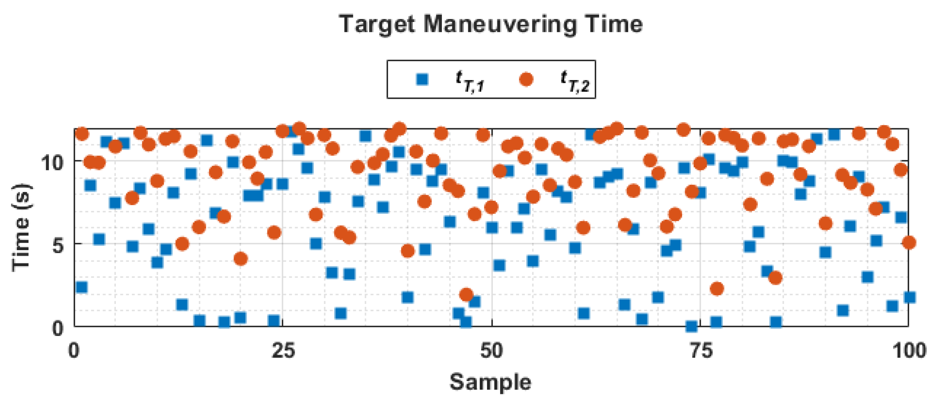
In this case, the initial target position was (−2000, 0) m and the heading angle was 180${}^{°}$. Figure 5 represents the first, i.e., $t_{T,1}$, and the second, i.e., $t_{T,2}$, maneuver time steps, when $t_{T,f}=12$ for 100 samples.

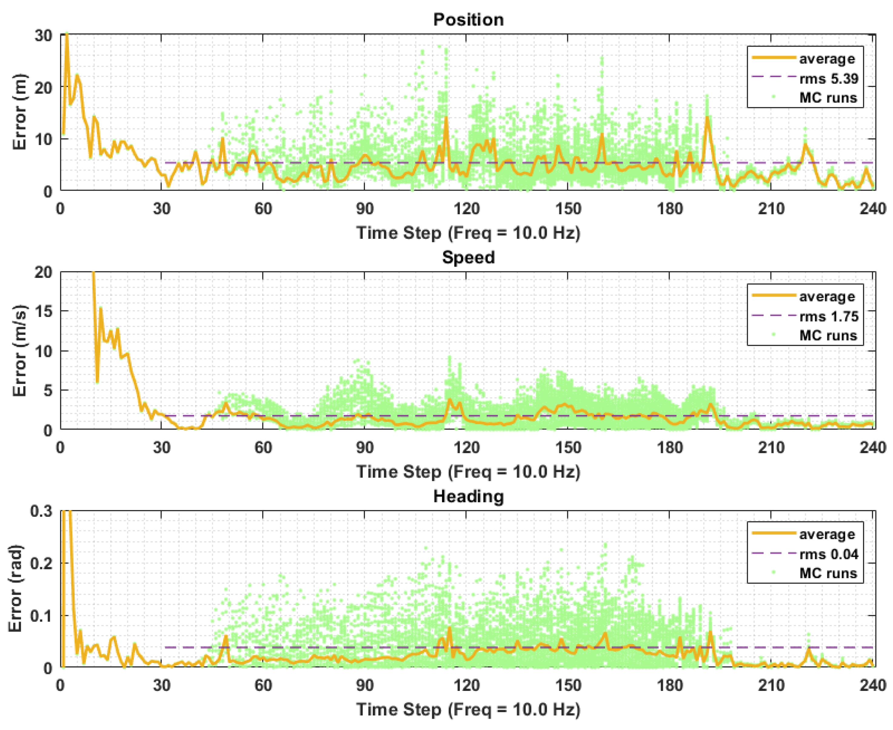
At the top of Figure 6, the average estimation error of the position is shown, and the RMS of the average error value is 5.39 m. The average estimation error of the speed is shown at the center of the figure, and the RMS of the error was about 1.75 m/s. In the middle, the average estimation error of the heading angles is shown. The RMS value of the error was 0.04 rad. Note that the estimation error was calculated as $e_k=\sqrt{{\left(x_k^{TRUE}-{\widehat{x}}_{k|k}\right)}^2}$, and the RMS values were calculated after the steady-state was reached.

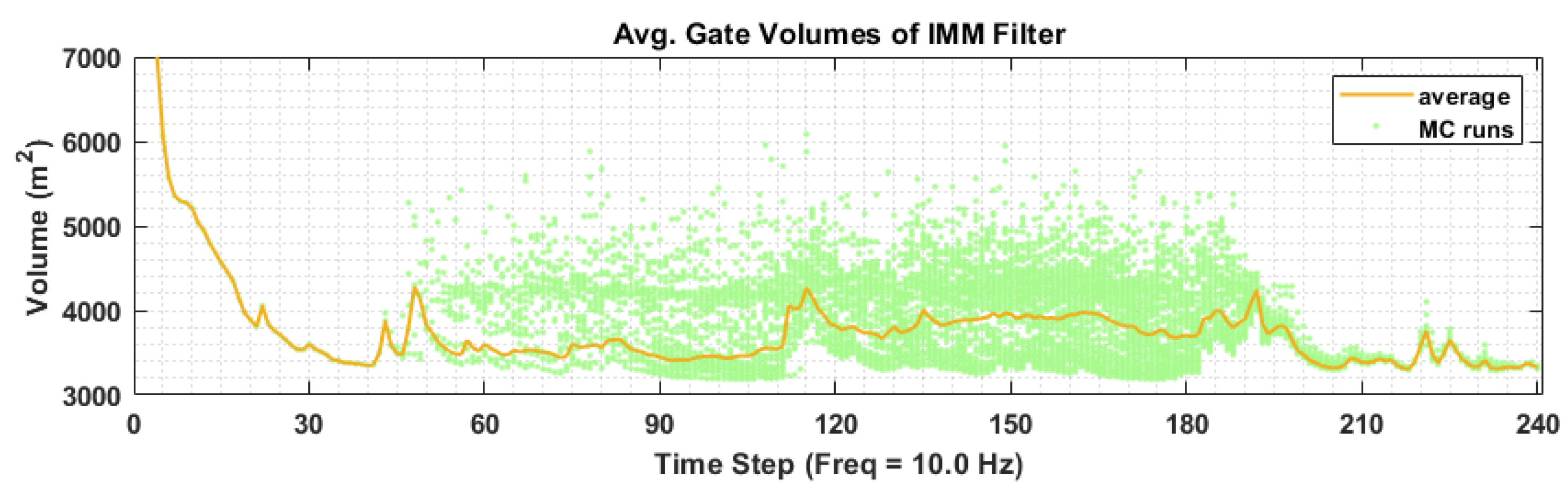
In Figure 7, the average gate volume of the IMM filter is shown. According to these figures, the IMM filter reached the steady-state after 3 s. The guidance algorithm was enabled after 4 s, and at that time, the target was located at (0, 0) with a 180${}^{°}$ heading angle. Therefore, the slant range was approximately 10 km when the guidance algorithm was initiated.

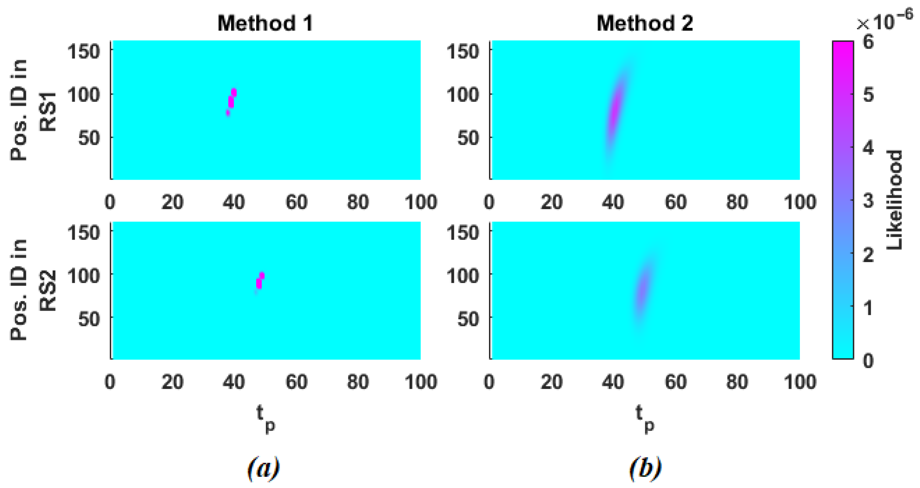
Figure 8 represents the likelihood of the reachable sets’ elements for the two methods as an example. In this figure, the horizontal axis represents the prediction time steps, and the vertical axis represents the position identity of the elements in the reachable set. According to the figure, the covariance of Method 1 was lower than Method 2 in this case. The covariance of Method 1 directly came from the measurement model; therefore, the covariance of Method 1 can be larger than Method 2.

In Figure 9, an example of the trajectories using Method 1 and Method 2 is shown. In this figure, the blue circle and square denote the target’s position when M1 and M2 are launched, respectively. The upward-pointing and downward-pointing triangles represent the interceptors’ positions when the target exhibits a maneuver for the first and second time, respectively.

The proposed algorithm was examined by varying the time bias to delay the launch, i.e., $\left(t_{\alpha }\in 3,5,7,9\right)$, the available interceptor numbers $\left(NoOfInt\in 1,2,3\right)$ for both target state prediction methods. By calculating the ratio of the number of interceptions to the number of simulations, the probability of interception was obtained.

In Figure 10, the probability of interception with respect to the miss distance is given for Method 1 and Method 2 when $t_{\alpha }$ is 7. In the case that Method 1 is used, the probability of interception is 42%, 62%, and 74%, for the one-to-one, two-to-one, and three-to-one scenarios, respectively. Note that $M1$ belongs to the one-to-one and $M1$ and $M2$ belong to the two-to-one scenarios. For Method 2, the probability of interception is 53%, 71%, and 82% for the same scenarios. These probabilities were calculated in the case of the lethal radius being 10 m. Increasing the number of interceptors improves the probability of interception dramatically. According to the results, knowing the target’s maneuverability limit provides an advantage over Method 1.

In Figure 11, the probability of interception is shown for different $t_{\alpha }$ values when the lethal radius is 10 m. When $t_{\alpha }=3$, Method 2 with two interceptors has a higher probability compared to Method 1 with three interceptors, although the number of interceptors is low. When $t_{\alpha }=9$, there is no significant difference between the probability of interception depending on the number of interceptors, although the highest probability was obtained. As $t_{\alpha }$ increases, the interceptors are launched much later. Hence, an increase in $t_{\alpha }$ may mean that the interceptors are launched after the target has completed its maneuver, and $M3$ may not improve the probability.

5.2. Case 2: Target Position ID Is 2

In this case, the initial target position is (−392.3, 6000) m, and the heading angle is 150${}^{°}$. The Monte Carlo simulations repeated the cooperation and prediction scenarios 100 times. Each repetition had randomly selected time instants for which the target exhibited a maneuver. The guidance algorithm was enabled after 4 s, and at that time, the target was located at (1339.7, 5000) with a 150${}^{°}$ heading angle. Therefore, the slant range was approximately 10 km when the guidance algorithm was initiated.

In Figure 12, the probability of interception is shown for different $t_{\alpha }$ values when the lethal radius is 10 m. When $t_{\alpha }=3$ and $t_{\alpha }=7$, Method 1 and Method 2 with two interceptors perform similarly. For all $t_{\alpha }$ values, the probability of interception increases as the interceptor number increases. When $t_{\alpha }=7$ and $t_{\alpha }=9$, Method 1 performs slightly better than Method 2.

5.3. Case 3: Target Position ID Is 3

In this case, initial target position is (4000, 10,392) m, and heading angle is 120${}^{°}$. The Monte Carlo simulations repeated the cooperation and prediction scenarios 100 times. Each repetition had randomly selected time instants that the target exhibited a maneuver. The guidance algorithm was enabled after 4 s, and at that time, the target was located at (5000, 8660.3) with a 120${}^{°}$ heading angle. Therefore, the slant range was approximately 10 km when the guidance algorithm was initiated.

In Figure 13, the probability of interception is shown for different $t_{\alpha }$ values when the lethal radius is 10 m. When $t_{\alpha }=3$, Method 1 and Method 2 with two interceptors perform similarly. For all $t_{\alpha }$ values, except $t_{\alpha }=3$, the probability of interception increases as the interceptor number increases. Although Method 1 slightly outperforms Method 2 when $t_{\alpha }=7$, Method 2 provides an overall increase in interception probability.

5.4. Case 4: Target Position ID Is 4

In this case, the initial target position was (10,000, 12,000) m, and the heading angle was 90${}^{°}$. The Monte Carlo simulations repeated the cooperation and prediction scenarios 100 times. Each repetition had randomly selected time instants that the target exhibited a maneuver. The guidance algorithm was enabled after 4 s, and at that time, the target was located at (10,000, 10,000) with a 90${}^{°}$ heading angle. Therefore, the slant range was approximately 10 km when the guidance algorithm was initiated.

In Figure 14, the probability of interception is shown for different $t_{\alpha }$ values when the lethal radius is 10 m. According to the results, increasing the interceptor number and knowledge about the target’s maneuverability limits increase the probability of interception, except when $t_{\alpha }=9$.

5.5. Results

The proposed cooperative guidance law was evaluated by altering the initial configurations of the interceptors, $t_{\alpha }$, and the knowledge about the target’s maneuverability limits. The simulation results showed that the proposed guidance law and target state prediction methods can effectively intercept a high-speed, high-maneuverability target, even with inferior interceptors. The algorithm’s performance remained successful despite varying the initial interceptor configurations. The results indicated that knowledge about the target’s maneuverability limits improved the interception probability in most cases, and the probability of interception increased with the number of interceptors. Additionally, the algorithm does not require target acceleration information.

Note that all calculations were performed at the ground station and the commands were sent to the interceptors, even though the computational cost of the proposed algorithm is high. The proposed algorithms were implemented using MATLAB R2017b, and the simulations were run using two parallel computers with an i5-4210U CPU @ 1.70GHz and 8.00GB RAM. It took approximately 5 h to run 100 simulations for a fixed interceptor velocity, $t_{\alpha }$, and prediction method.

6. Conclusions

This paper presented a novel cooperative and predictive guidance law for intercepting high-speed, high-maneuverability targets with inferior interceptors. The goal of the guidance law was to cooperatively cover the most-probable future locations of the target. To achieve this, the predicted target state was expressed as a probability density function, and the likelihood of the deterministic reachable set of elements of the interceptors was calculated based on this predicted state. The paper proposed two methods for predicting the target state, depending on the knowledge of the target’s maneuverability limit. The simulation results showed that the proposed algorithm performed well against targets exhibiting effective maneuvering, even if the maneuvering capabilities of the interceptors were lower than those of the target. Additionally, the algorithm’s performance remained successful despite varying the initial interceptor configurations. It was also shown that knowledge of the target’s maneuverability limit increased the probability of interception. The proposed algorithm did not have strict constraints on the initial state of the interceptors and was tested using simulation parameters that were close to real-world applications. Future work will involve a more complex engagement model that takes into account the three-dimensional kinematics, the variable speeds of the interceptors and the target, and additional target maneuvering modes.

References

- Zarchan, P. Tactical and Strategic Missile Guidance; American Institute of Aeronautics and Astronautics, Inc.: Reston, VA, USA, 2012. [Google Scholar]
- Jeon, I.S.; Lee, J.I.; Tahk, M.J. Impact-time-control guidance law for anti-ship missiles. IEEE Trans. Control Syst. Technol. 2006, 14, 260–266. [Google Scholar] [CrossRef]
- Lee, J.I.; Jeon, I.S.; Tahk, M.J. Guidance law to control impact time and angle. IEEE Trans. Aerosp. Electron. Syst. 2007, 43, 301–310. [Google Scholar]
- Harl, N.; Balakrishnan, S. Impact time and angle guidance with sliding mode control. IEEE Trans. Control Syst. Technol. 2011, 20, 1436–1449. [Google Scholar] [CrossRef]
- Kim, M.; Jung, B.; Han, B.; Lee, S.; Kim, Y. Lyapunov-based impact time control guidance laws against stationary targets. IEEE Trans. Aerosp. Electron. Syst. 2015, 51, 1111–1122. [Google Scholar] [CrossRef]
- Saleem, A.; Ratnoo, A. Lyapunov-based guidance law for impact time control and simultaneous arrival. J. Guid. Control. Dyn. 2016, 39, 164–173. [Google Scholar] [CrossRef]
- Shiyu, Z.; Rui, Z. Cooperative guidance for multimissile salvo attack. Chin. J. Aeronaut. 2008, 21, 533–539. [Google Scholar] [CrossRef]
- Jeon, I.S.; Lee, J.I.; Tahk, M.J. Homing guidance law for cooperative attack of multiple missiles. J. Guid. Control Dyn. 2010, 33, 275–280. [Google Scholar] [CrossRef]
- Hou, D.; Wang, Q.; Sun, X.; Dong, C. Finite-time cooperative guidance laws for multiple missiles with acceleration saturation constraints. IET Control Theory Appl. 2015, 9, 1525–1535. [Google Scholar] [CrossRef]
- Zhao, J.; Zhou, R.; Dong, Z. Three-dimensional cooperative guidance laws against stationary and maneuvering targets. Chin. J. Aeronaut. 2015, 28, 1104–1120. [Google Scholar] [CrossRef]
- Zhang, Y.; Ma, G.; Wang, X. Time-cooperative guidance for multi-missiles: A leader–follower strategy. Acta Aeronaut. Astronaut. Sin. 2009, 30, 1109–1118. [Google Scholar]
- Shiyu, Z.; Rui, Z.; Chen, W.; Quanxin, D. Design of time-constrained guidance laws via virtual leader approach. Chin. J. Aeronaut. 2010, 23, 103–108. [Google Scholar]
- Li, G.; Li, Q.; Wu, Y.; Xu, P.; Liu, J. Leader-following cooperative guidance law with specified impact time. Sci. China Technol. Sci. 2020, 63, 2349–2356. [Google Scholar] [CrossRef]
- Wang, Z.; Fu, W.; Fang, Y.; Zhu, S.; Wu, Z.; Wang, M. Prescribed-time cooperative guidance law against maneuvering target based on leader-following strategy. ISA Trans. 2022, 129, 257–270. [Google Scholar] [CrossRef]
- Sun, X.; Zhou, R.; Hou, D.; Wu, J. Consensus of leader–followers system of multi-missile with time-delays and switching topologies. Optik 2014, 125, 1202–1208. [Google Scholar] [CrossRef]
- Zhao, J.; Zhou, R. Unified approach to cooperative guidance laws against stationary and maneuvering targets. Nonlinear Dyn. 2015, 81, 1635–1647. [Google Scholar]
- Nikusokhan, M.; Nobahari, H. Closed-form optimal cooperative guidance law against random step maneuver. IEEE Trans. Aerosp. Electron. Syst. 2016, 52, 319–336. [Google Scholar]
- Shaferman, V.; Shima, T. Cooperative differential games guidance laws for imposing a relative intercept angle. J. Guid. Control Dyn. 2017, 40, 2465–2480. [Google Scholar] [CrossRef]
- Zhou, J.; Lü, Y.; Li, Z.; Yang, J. Cooperative guidance law design for simultaneous attack with multiple missiles against a maneuvering target. J. Syst. Sci. Complex. 2018, 31, 287–301. [Google Scholar] [CrossRef]
- Wang, X.H.; Tan, C.P. 3-D impact angle constrained distributed cooperative guidance for maneuvering targets without angularrate measurements. Control Eng. Pract. 2018, 78, 142–159. [Google Scholar]
- Zhao, Q.; Dong, X.; Song, X.; Ren, Z. Cooperative time-varying formation guidance for leader-following missiles to intercept a maneuvering target with switching topologies. Nonlinear Dyn. 2019, 95, 129–141. [Google Scholar]
- Yu, J.; Dong, X.; Li, Q.; Ren, Z. Distributed cooperative encirclement hunting guidance for multiple flight vehicles system. Aerosp. Sci. Technol. 2019, 95, 105475. [Google Scholar] [CrossRef]
- Jing, L.; Zhang, L.; Guo, J.; Cui, N. Fixed-time cooperative guidance law with angle constraint for multiple missiles against maneuvering target. IEEE Access 2020, 8, 73268–73277. [Google Scholar]
- Zhai, S.; Wei, X.; Yang, J. Cooperative guidance law based on time-varying terminal sliding mode for maneuvering target with unknown uncertainty in simultaneous attack. J. Frankl. Inst. 2020, 357, 11914–11938. [Google Scholar]
- Chen, Z.; Chen, W.; Liu, X.; Cheng, J. Three-dimensional fixed-time robust cooperative guidance law for simultaneous attack with impact angle constraint. Aerosp. Sci. Technol. 2021, 110, 106523. [Google Scholar]
- Liu, F.; Dong, X.; Li, Q.; Ren, Z. Robust multi-agent differential games with application to cooperative guidance. Aerosp. Sci. Technol. 2021, 111, 106568. [Google Scholar]
- Dong, X.; Ren, Z. Finite-time distributed leaderless cooperative guidance law for maneuvering targets under directed topology without numerical singularities. Aerospace 2022, 9, 157. [Google Scholar] [CrossRef]
- Su, W.; Li, K.; Chen, L. Coverage-based cooperative guidance strategy against highly maneuvering target. Aerosp. Sci. Technol. 2017, 71, 147–155. [Google Scholar] [CrossRef]
- Su, W.; Shin, H.S.; Chen, L.; Tsourdos, A. Cooperative interception strategy for multiple inferior missiles against one highly maneuvering target. Aerosp. Sci. Technol. 2018, 80, 91–100. [Google Scholar] [CrossRef]
- Su, W.; Li, K.; Chen, L. Coverage-based three-dimensional cooperative guidance strategy against highly maneuvering target. Aerosp. Sci. Technol. 2019, 85, 556–566. [Google Scholar] [CrossRef]
- Wang, L.; Liu, K.; Yao, Y.; He, F. A design dpproach for simultaneous cooperative interception based on area coverage optimization. Drones 2022, 6, 156. [Google Scholar] [CrossRef]
- Yan, X.; Kuang, M.; Zhu, J.; Yuan, X. Reachability-based cooperative strategy for intercepting a highly maneuvering target using inferior missiles. Aerosp. Sci. Technol. 2020, 106, 106057. [Google Scholar] [CrossRef]
- Ziyan, C.; Jianglong, Y.; Xiwang, D.; Zhang, R. Three-dimensional cooperative guidance strategy and guidance law for intercepting highly maneuvering target. Chin. J. Aeronaut. 2021, 34, 485–495. [Google Scholar]
- Zhang, B.; Zhou, D.; Li, J.; Yao, Y. Coverage-based cooperative guidance strategy by controlling flight path angle. J. Guid. Control Dyn. 2022, 45, 972–981. [Google Scholar] [CrossRef]
- Best, R.; Norton, J. Predictive missile guidance. J. Guid. Control Dyn. 2000, 23, 539–546. [Google Scholar]
- Shaviv, I.; Oshman, Y. Guidance without assuming separation. In Proceedings of the AIAA Guidance, Navigation, and Control Conference and Exhibit, San Francisco, CA, USA, 15–18 August 2005; p. 6154. [Google Scholar]
- Dionne, D.; Michalska, H.; Rabbath, C.A. A predictive guidance law with uncertain information about the target state. In Proceedings of the 2006 American Control Conference, Minneapolis, MN, USA, 14–16 June 2006; IEEE: Piscataway, NJ, USA, 2006; pp. 1062–1067. [Google Scholar]
- Dionne, D.; Michalska, H.; Rabbath, C. Predictive guidance for pursuit-evasion engagements involving multiple decoys. J. Guid. Control Dyn. 2007, 30, 1277–1286. [Google Scholar]
- Li, X.R.; Jilkov, V.P. Survey of maneuvering target tracking. Part I. Dynamic models. IEEE Trans. Aerosp. Electron. Syst. 2003, 39, 1333–1364. [Google Scholar]
- Mallick, M.; La Scala, B. Comparison of single-point and two-point difference track initiation algorithms using position measurements. Acta Autom. Sin. 2008, 34, 258–265. [Google Scholar]
- Bar-Shalom, Y.; Li, X.R.; Kirubarajan, T. Estimation with Applications to Tracking and Navigation: Theory Algorithms and Software; John Wiley & Sons: Hoboken, NJ, USA, 2004. [Google Scholar]
Figure 1.
Planar engagement geometry.
Figure 2.
Illustration of reachable sets, corresponding likelihood, and pdf of predicted target state when time instants (a) , (b) , and (c) .
Figure 3.
Flow diagram of the proposed cooperative guidance law.
Figure 4.
Initial position configurations of the target.
Figure 5.
Target maneuvering time instants.
Figure 6.
Average estimation errors.
Figure 7.
Average gate volume of IMM filter.
Figure 8.
An example of the likelihood of reachable sets where , MC Run No. 71. (a) Method 1, (b) Method 2.
Figure 9.
An example of trajectories where , m/s, MC Run No. 71. (a) Method 1, (b) Method 2.
Figure 10.
The probability of interception, .
Figure 11.
Comparison of the probability of interception for all , in Case 1.
Figure 12.
Comparison of probability of interception for all , in Case 2.
Figure 13.
Comparison of probability of interception for all , in Case 3.
Figure 14.
Comparison of probability of interception for all , in Case 4.
Disclaimer/Publisher’s Note: The statements, opinions and data contained in all publications are solely those of the individual author(s) and contributor(s) and not of MDPI and/or the editor(s). MDPI and/or the editor(s) disclaim responsibility for any injury to people or property resulting from any ideas, methods, instructions or products referred to in the content. |
© 2023 by the authors. Licensee MDPI, Basel, Switzerland. This article is an open access article distributed under the terms and conditions of the Creative Commons Attribution (CC BY) license (https://creativecommons.org/licenses/by/4.0/).
Share and Cite
MDPI and ACS Style
Cevher, F.Y.; Leblebicioğlu, M.K. Cooperative Guidance Law for High-Speed and High-Maneuverability Air Targets. Aerospace 2023, 10, 155. https://doi.org/10.3390/aerospace10020155
AMA Style
Cevher FY, Leblebicioğlu MK. Cooperative Guidance Law for High-Speed and High-Maneuverability Air Targets. Aerospace. 2023; 10(2):155. https://doi.org/10.3390/aerospace10020155
Chicago/Turabian StyleCevher, Fırat Yılmaz, and Mehmet Kemal Leblebicioğlu. 2023. "Cooperative Guidance Law for High-Speed and High-Maneuverability Air Targets" Aerospace 10, no. 2: 155. https://doi.org/10.3390/aerospace10020155
Note that from the first issue of 2016, this journal uses article numbers instead of page numbers. See further details here.