
AILC for Rigid-Flexible Coupled Manipulator System in Three-Dimensional Space with Time-Varying Disturbances and Input Constraints
School of Automation, Guangxi University of Science and Technology, Liuzhou 545000, China
*
Author to whom correspondence should be addressed.
Actuators 2022, 11(9), 268; https://doi.org/10.3390/act11090268
Submission received: 28 August 2022
/
Revised: 15 September 2022
/
Accepted: 16 September 2022
/
Published: 19 September 2022
(This article belongs to the Special Issue Intelligent Control of Flexible Manipulator Systems and Robotics)
Abstract
:In this paper, an adaptive iterative learning control (AILC) law is developed for two-link rigid-flexible coupled manipulator system in three-dimensional (3D) space with time-varying disturbances and input constraints. Based on the Hamilton’s principle, a dynamic model of a manipulator system is established. The conditional equation that is coupled by ordinary differential equations and partial differential equations is derived. In order to achieve high-precision tracking of the revolving angles and vibration suppression of the elastic part, the iterative learning control law based on the disturbance observer is considered in the process of the design controller. The composite Lyapunov energy function is proposed to prove that the angle errors and elastic deformation can eventually converge to zero with the increase of the number of iterations. Ultimately, the simulation results to rigid-flexible coupled manipulator system are given to prove the convergence of the control objectives under the adaptive iterative learning control law.
1. Introduction
In the past few years, robotic manipulator systems have been widely employed in a range of fields reminiscent of military, industry, aerospace satellites, ocean exploration, and so on [1,2,3,4,5,6,7,8,9]. The rigid manipulator has the characteristics of a high degree of freedom and wide practicability [10]. Compared with the rigid manipulator, the flexible manipulator has the characteristics of low energy consumption and high flexibility. It also has wide application range [11,12,13,14]. Meanwhile, the necessities for performance indicators of manipulator like flexibility and low energy consumption are needed increasingly; flexible robotic manipulators are not fully competent in some special practical situations. Recently, the rigid-flexible robotic manipulator has additionally gotten a lot of attention [15,16]. The rigid-flexible coupling manipulator has the advantages of lighter weight and higher flexibility, and can be used in more practical occasions [17]. In the past few years, there have been many studies on rigid-flexible coupled manipulators. In [18], it was the first time that the dynamic model of the two-link rigid-flexible manipulator system was derived. Within the years that followed, various control methods were investigated, such as boundary control [17,19,20], adaptive control [21], tip position control [22], nonlinear control [23], optimal control [12], and so on. The control methods mentioned above have the advantages of strong adaptability and wide application, however, they cannot achieve the purpose of completely tracking the control target in limited time. For this reason, the control method of iterative learning control is chosen in this paper.
Iterative learning control (ILC) is a new kind of learning control strategy, which can deal with some non-linear, complicated, and difficult models in a simple way [24]. It is suitable for performing repeatable tasks, and its goal is to improve tracking performance by using the error of the previous iteration into the input of the next iteration control [25]. It has superb significance for resolving high-precision trajectory tracking and control issues. Recently, a variety of iterative learning controllers attached to the rigid-flexible robotic manipulator were developed. In [26], a kind of iterative learning boundary control law is implemented on the two-link rigid-flexible coupled manipulator system. Authors derived the dynamic model of system by using Hamilton’s principle. Finally, the simulation results verify its effectiveness and realize the high-precision tracking effect. In [27], the authors studied a disturbance observer-based adaptive boundary iterative learning control method that was used for two-link rigid-flexible coupled manipulator system. More than that, the condition of endpoint constraint and input backlash situation were considered. Finally, the convergence analysis was performed by combining the barrier Lyapunov function. In [27], the author developed a more complex external situation in which distributed disturbance and input constraints were further considered. The control objectives were achieved by using the iterative learning control law, which is combined with hyperbolic tangent and saturation functions.
The above-referred studies about two-link rigid-flexible manipulator were particularly accomplished in the two-dimensional space. Different from the three-link manipulator, the model described in this paper adds a rotating base on the basis of the two-link rigid-flexible coupling manipulator, so that it can move in three-dimensional space. In actual application, 3D manipulators have more application scenarios than planar manipulators, can solve more practical problems, and have longer-term significance of research [28]. However, there are few related studies, and it is more difficult than the traditional two-dimensional model. In the latest years, research on the 3D two-link rigid-flexible coupled manipulator has also gradually appeared in the field of researchers. In [29], the authors modeled the manipulator system based on infinite-dimensional nonlinear model, and the tracking problem of the system that has actuator faults is solved by using boundary control method in three-dimensional space. In [30], the authors proposed the research of the control problem under input saturation. It should be mentioned that no studies have been reported about the control method of iterative learning to 3D rigid-flexible manipulator, which is a research direction really well worth considering. However, the related research on iterative learning of rigid-flexible coupled manipulators in three-dimensional space has not been published so far.
In this paper, we designed an adaptive iterative learning control method to solve the control problems of the rigid-flexible manipulator in 3D space. Firstly, the dynamic model of the system is derived through using Hamilton’s principle. On the premise of composite Lyapunov energy function and Young’s inequality theory, the angular error and elastic deformation can ultimately converge to zero with the increase of the number of iterations. The most important contributions are summarized below:
- (1)
- This paper is the first work regarding the two-link rigid-flexible manipulator system in 3D space by using adaptive iterative learning control. In the controller design section, the adaptive iterative learning control law is designed based on observers.
- (2)
- By designing the composite Lyapunov energy function, combined with Young’s inequality, the convergence of angular error and elastic deformation will be proved strictly.
The article is organized as follows: The dynamic model of the rigid-flexible coupled manipulator in 3D space is presented in Section 2. The adaptive iterative learning control law and convergence analysis are given in Section 3. Simulation results of the control law are shown in Section 4. Finally, the conclusion of this paper is given in Section 5.
2. System Description and Control Objectives
2.1. System Description
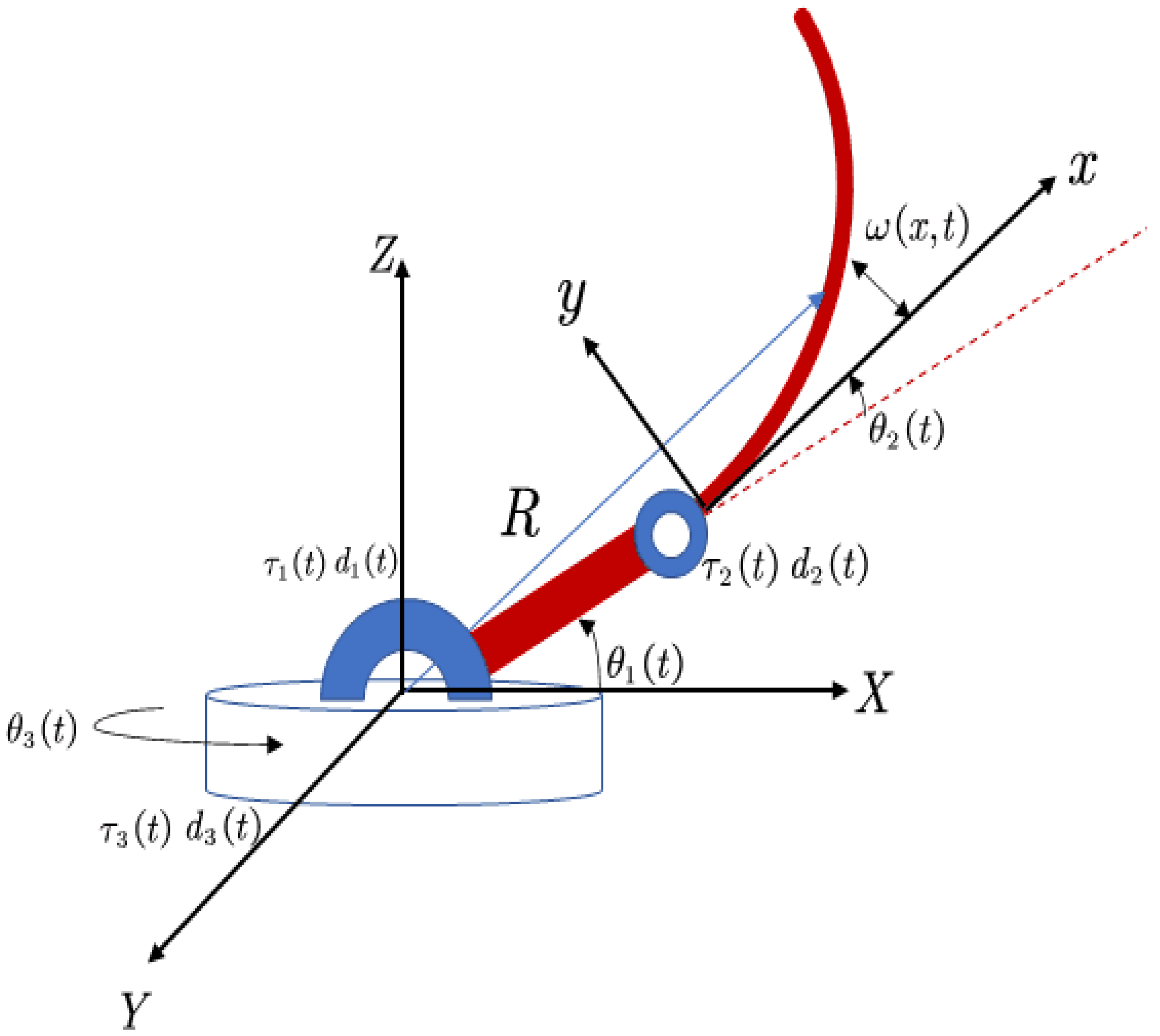
A three-dimensional(3D) two-link rigid-flexible coupling manipulator system is shown in Figure 1 [29]. It consists of a rotating shaft base, rigid and flexible links, and two joints, and the rotating shaft base can be rotated on the horizontal plane. The three actuators named , , and are located in the rigid and flexible links and the rotating shaft base, respectively. represents the angular position of the rigid link, indicates the angular position of the flexible link, is the angular position of the rotating shaft base, which is measured from the counterclockwise of X-axis. At the same time, are the time-varying disturbances of the system. is the moment of inertia of the joint, which is relative to the rigid part of system at the shoulder position; is the moment of inertia of the joint, which is relative to the flexible part of system at the elbow position; is the moment of inertia of the rotatable base relative to the Z-axis; is the quality of every joint; is the density of the flexible part; is the length of the rigid link; is the length of the flexible link; is the uniform flexural rigidity of the flexible link; and is the elastic deformation variable of the flexible link that changes over time.
For the sake of using the Hamilton’s principle, we can obtain the dynamic equations of two-link rigid-flexible coupled manipulator system in three-dimensional space [18]. In this paper, the dynamic equations are simplified below:
where, , , , , and , , are defined as:
with .
Remark 1.
In this article, for clarity, the notations are described as follows:,,,,and, respectively.
In Formula (1), represents the time-varying disturbances to the system, and the condition of input constraint is defined as: , and there is:
where is defined as the upper bound of .
At the same time, the coupled PDE-ODE equation of system is given as:
And natural boundary conditions of the system are expressed as:
Remark 2.
Different from [29], in this paper, in order to deal with the problems that the manipulator may encounter in the actual working environment, the input constraint problem and the time-varying disturbance problem are considered in the dynamic model of the system.
2.2. Control Objectives
In order to achieve the high-precision tracking of the joints’ angle and vibration suppression of the elastic manipulator part [31], control objectives for the 3D rigid-flexible coupled manipulator system can be shown as:
3. The Design of Adaptive Iterative Learning Controller and Convergence Analysis
For ensuring the following content is rigorous, the assumptions are created concerning the 3D rigid-flexible coupled manipulator system before designing the adaptive iterative learning control law. The following assumptions are proposed:
A1: Joint position angle and elastic deformation can be measured and used for feedback.
A2: The target angle is bounded in finite time , and are slow-varying or constants.
A3: The unknown time-varying disturbances are bounded, and , where
is constant and .
A4: Each iteration process has the same initial condition, that is, , used to secure the tracking performance of the system.
A5: The kinetic energy of system is bounded for .
3.1. The Design of Adaptive Iterative Learning Control Law
The adaptive iterative learning controller is designed as:
where , , and are constants, , and , .
So in order to cope with the conditions of the input constraints, the iterative learning control law, which is based on hyperbolic tangent function, is designed:
where , , , , and are constants, and .
Remark 3.
In the control law (10)–(15), we use the hyperbolic tangent function to design the controller. In previous studies, the sign function is commonly used in the design of controllers. The use of sign function makes the design of the controller simpler and more efficient, but it leads to undesired chattering in the tracking trajectory [26]. By using the hyperbolic tangent function, one can effectively avoid this phenomenon.
3.2. Convergence Analysis
In the convergence analysis part, the convergence of the rigid-flexible coupled manipulator system is proved by composite Lyapunov function stability theory [33].
Firstly, let and .
The composite Lyapunov energy function is constructed as follows [26]:
Remark 4.
In [26], a composite Lyapunov function is designed for the rigid-flexible coupled manipulator system in two-dimensional space to verify the convergence. In this paper, it is improved and the composite Lyapunov function in three-dimensional space for the system is designed.
Among them, stands for:
where R is the position vector of the general points in the global inertial coordinate system and R is expressed as:
The proof process is split into the subsequent three steps to prove the convergence of angle error and elastic deformation.
Step 1: To prove the non-increasing property of the composite Lyapunov energy function along the iterative axis.
From (19), we have:
In the same manner, we can further get:
and
From (19), we can also get:
which is
Similarly, the following inequality can be obtained:
After that, the time derivative of Equation (20) can be expressed as:
Substituting the dynamic model of the system into (28), one has:
Meanwhile, in accordance with the Newton-Leibniz formula, the form of can be rewritten as:
Then, the following equation holds:
By utilizing (10)–(12) to Equation (31), one can obtain:
Further, we can get:
Next, we calculate the difference of the composite Lyapunov function by using the above equations; the following inequality can be obtained:
Since the saturation function has the property that: if , and , are continuous [7], then there is:
By substituting Equation (35) into Equation (34), we can further derive:
By Formula (36), it can be proved that is non-increasing.
Step 2: To prove that the first term of the composite Lyapunov energy function is bounded.
It can be calculated from Equation (19):
Then, one can obtain:
Invoking (16)–(18) and calculating leads to:
and
From the disturbance observers (13)–(15) and , it can be obtained that:
By utilizing (39)–(43) to (38), it yields:
Then, it is not hard to get:
By using the Young’s inequality, which yields:
where are constants and .
Subsequently, substituting (46)–(48) into (45), it can be easily calculated as:
Until now, the boundedness of has been proven.
Step 3: To analyze the convergence property of the angular errors and the deformation of flexible part of manipulator along the iterative axis.
Firstly, rewriting the as:
So, the following inequality can be given:
Then, according to (51), one has:
So, the above procedure can demonstrate that is bounded for and .
To sum up, we can see that the control objectives can be verified by adaptive iterative learning control law through the proving process.
4. Simulations
In this section, we perform several numerical simulations on a two-link rigid-flexible coupled manipulator that has the condition of input constraints and time-varying disturbances in three-dimensional space. The results of simulations give an intuitive description of the effectiveness of the system, which is projected adaptive iterative learning control law (10)–(12). The parameters of the system are given in Table 1 and the parameters of adaptive iterative learning control law are listed in Table 2.
Remark 5.
In [27,29,30], the authors studied the related research of two-link rigid-flexible coupling manipulator and the relevant simulation results are given. The parameters in Table 1 and Table 2 are further modified and tried from the parameters in the references to make it more in line with the adaptive iterative learning control law in this paper.
Firstly, setting the time step to , the space step is set to and the number of iterations is set to 15, respectively. Secondly, we define that desired angle as: , , and the time-varying disturbances are set as: , , and , respectively. The problem of input saturation is not considered in the simulation.
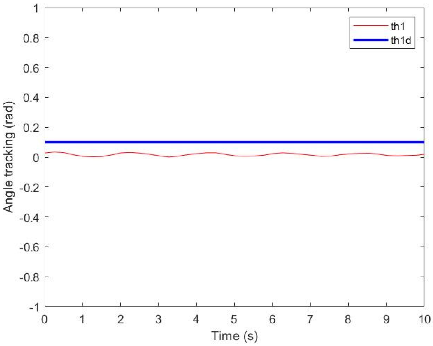
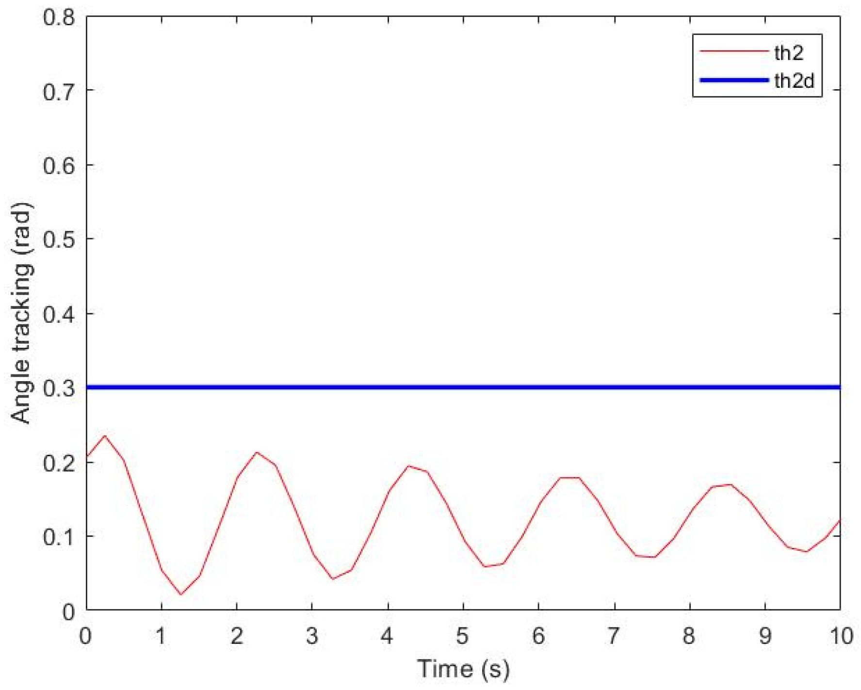
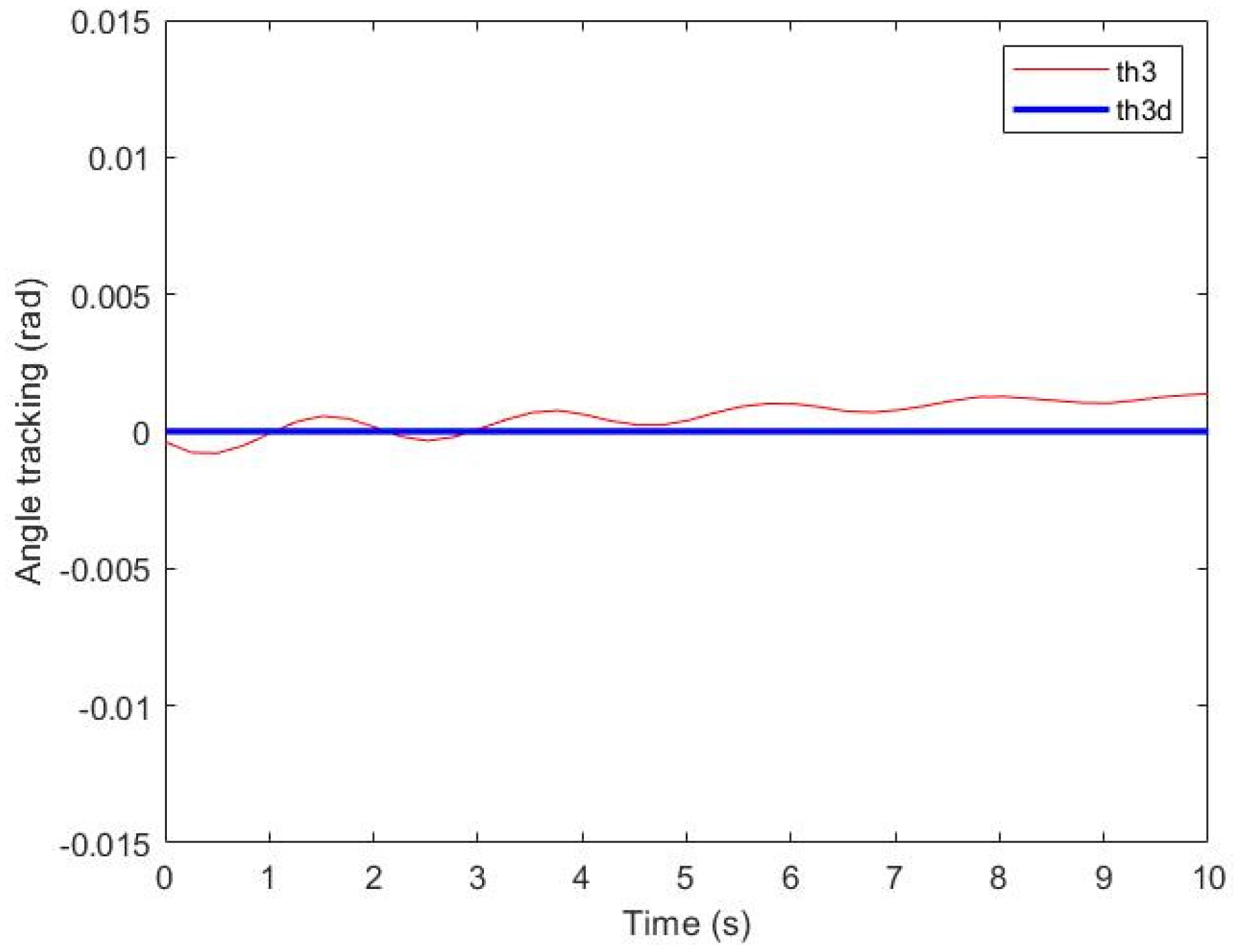
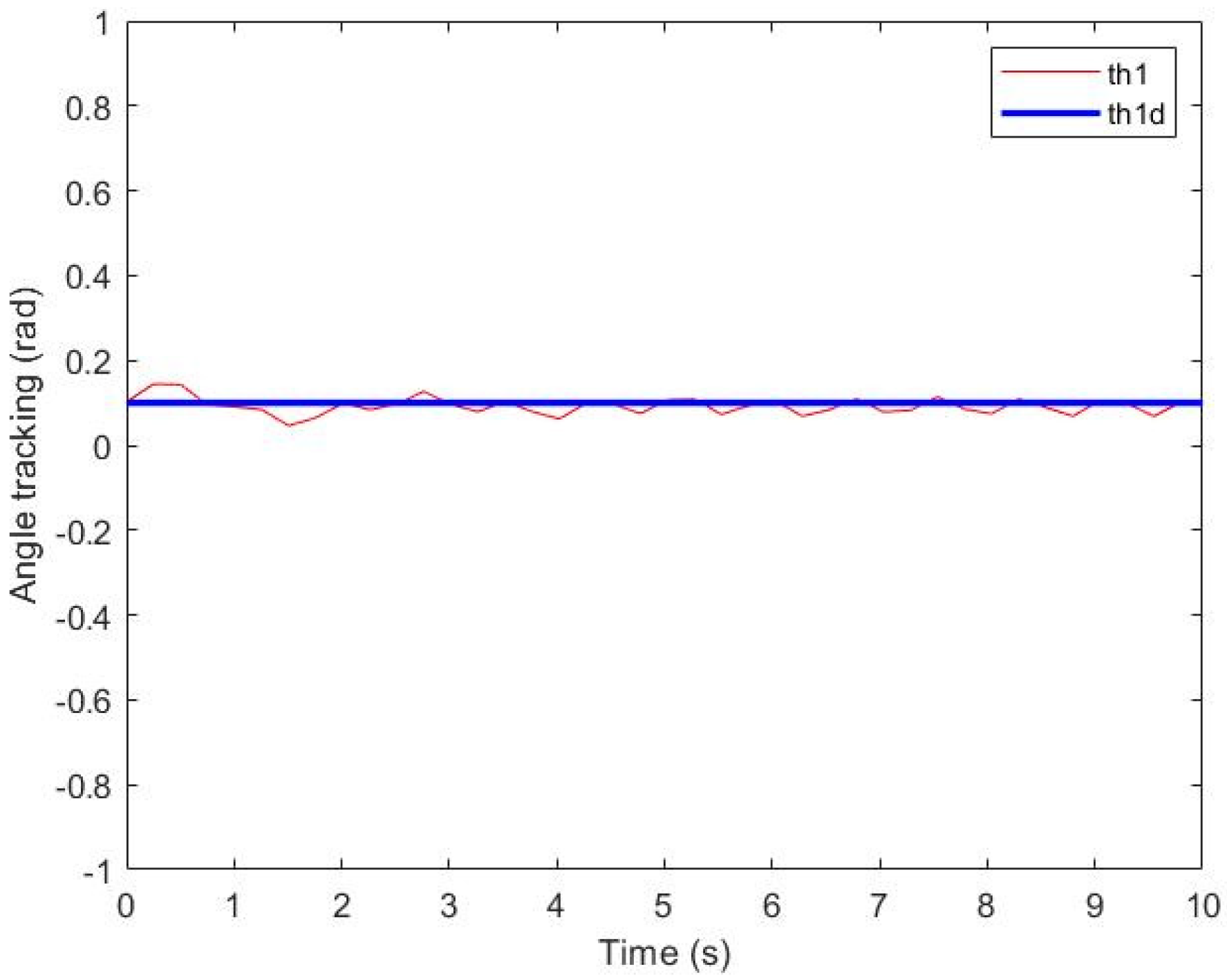
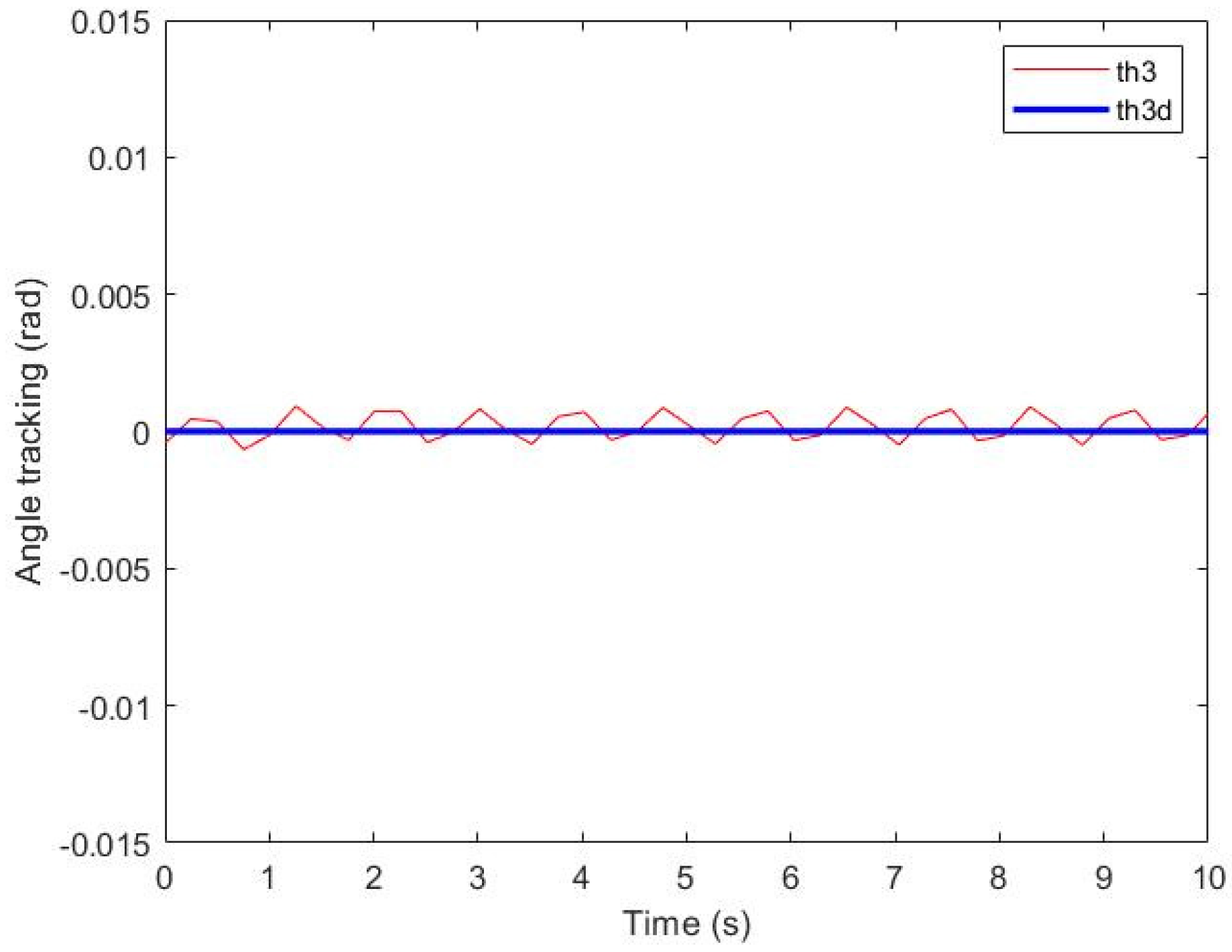
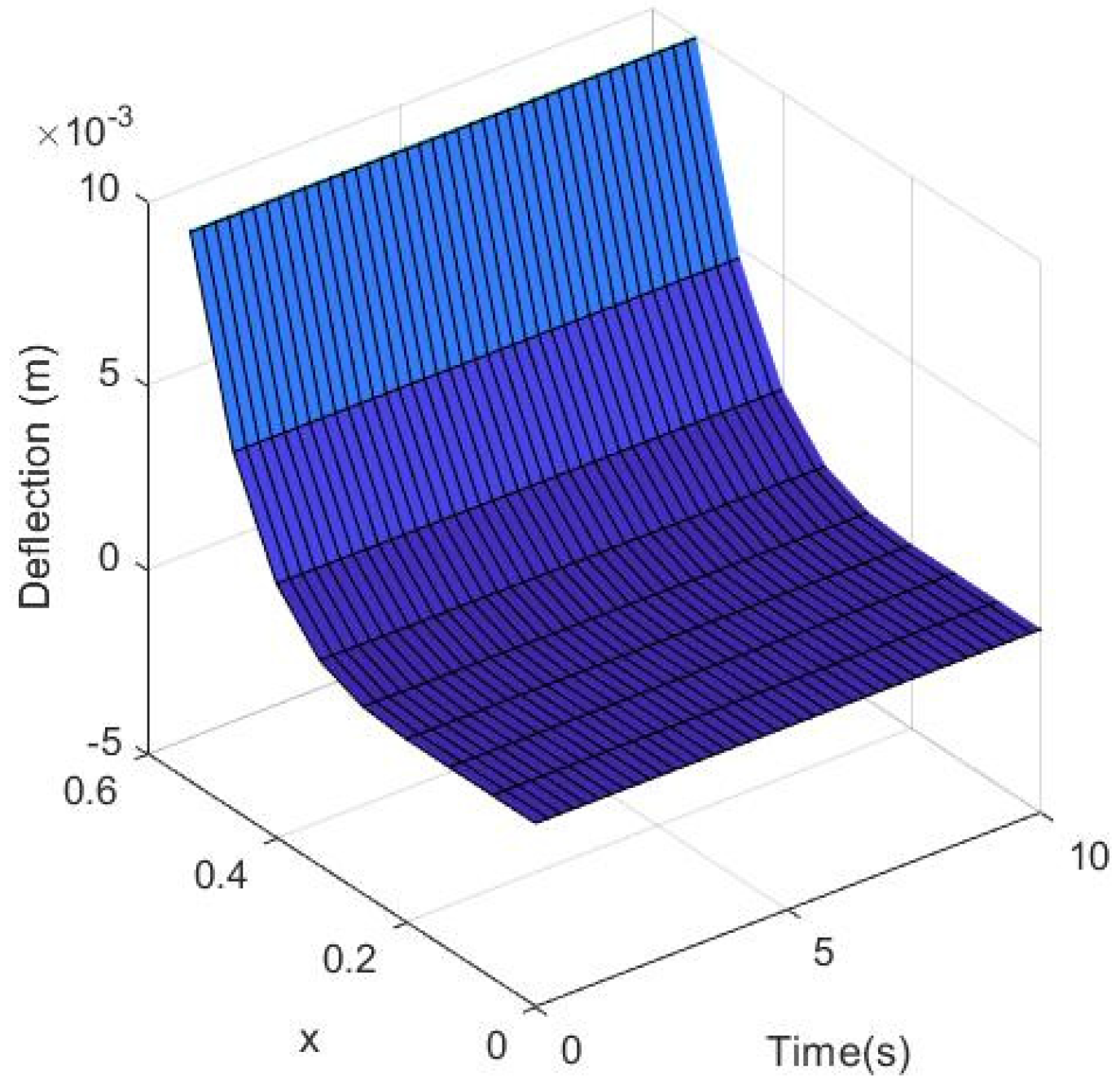
In Figure 2, Figure 3, Figure 4, Figure 5, Figure 6 and Figure 7, the simulation results show the performance of angle tracking for three angles before and after applying the adaptive iterative learning control law. From the figures we can see that the control law has an obvious effect on the convergence of the angle tracking. Similarly, in Figure 8 and Figure 9, it can be seen that the control law is also very effective in suppressing elastic deformation. In summary, the simulation results demonstrate the effectiveness of the adaptive control law.
5. Conclusions
This paper studied the two-link rigid-flexible coupled manipulator in three-dimensional (3D) space with time-varying disturbances and input constraints. Furthermore, in the process of the designing of control law, we proposed an adaptive iterative learning law based on disturbance observers and dealing with the conditions of the input constraints by using hyperbolic tangent function. By considering the composite Lyapunov function stability theory, we proved thar the angle error and the value of the elastic deformation variable are convergent. Through the simulation results, the effect of angle tracking and elastic suppression before and after applying the adaptive iterative learning control law to the system are compared. The effectiveness of the control law is further illustrated. Our future research direction is in the improvement of response time and optimizing the control law for the system in three-dimensional space, in addition, we will try to compare the results of different control methods together.
Author Contributions
Writing—original draft preparation, J.Z.; writing—review and editing, X.D.; visualization, Q.H.; supervision, Q.W. All authors have read and agreed to the published version of the manuscript.
Funding
This research was funded by National Nature Science Foundation of China (Grant No. 61863004); the Science and Technology Plan Projects of Liuzhou (Grant No. 2021AAF0103); the Innovation Project of Guangxi University of Science and Technology Graduate Education (Grant No. GKYC202225); the Innovation Project of Guangxi Graduate Education (No. YCSW2022436); the Science and Technology Association Projects of Liuzhou (No. 20210104).
Conflicts of Interest
The authors declare no conflict of interest.
References
- Cao, F.; Liu, J. Vibration control for a rigid-flexible manipulator with full state constraints via Barrier Lyapunov Function. J. Sound Vib. 2017, 406, 237–252. [Google Scholar] [CrossRef]
- He, W.; Meng, T.; Huang, D.; Li, X. Adaptive Boundary Iterative Learning Control for an Euler-Bernoulli Beam System With Input Constraint. IEEE Trans. Neural Netw. Learn. Syst. 2017, 29, 1539–1549. [Google Scholar] [CrossRef] [PubMed]
- He, W.; He, X.; Zou, M.; Li, H. PDE Model-Based Boundary Control Design for a Flexible Robotic Manipulator with Input Backlash. IEEE Trans. Control Syst. Technol. 2018, 27, 790–797. [Google Scholar] [CrossRef]
- Guo, F.; Liu, Y.; Wu, Y.; Luo, F. Observer-based backstepping boundary control for a flexible riser system. Mech. Syst. Signal Process. 2018, 111, 314–330. [Google Scholar] [CrossRef]
- Endo, T.; Sasaki, M.; Matsuno, F.; Jia, Y. Contact-Force Control of a Flexible Timoshenko Arm in Rigid/Soft Environment. IEEE Trans. Autom. Control 2017, 62, 2546–2553. [Google Scholar] [CrossRef]
- Liu, Z.; Liu, J.; He, W. Modeling and vibration control of a flexible aerial refueling hose with variable lengths and input constraint. Automatica 2017, 77, 302–310. [Google Scholar] [CrossRef]
- He, W.; Meng, T.; Zhang, S.; Liu, J.K.; Li, G.; Sun, C. Dual-Loop Adaptive Iterative Learning Control for a Timoshenko Beam with Output Constraint and Input Backlash. IEEE 2019, 49, 1027–1038. [Google Scholar] [CrossRef]
- Yabuno, H.; Kobayashi, S. Motion control of a flexible underactuated manipulator using resonance in a flexible active arm. Int. J. Mech. Sci. 2020, 174, 105432. [Google Scholar] [CrossRef]
- Zhao, Z.; Ahn, C.K. Boundary Output Constrained Control for a Flexible Beam System with Prescribed Performance. IEEE Trans. Syst. Man Cybern. Syst. 2021, 51, 4650–4658. [Google Scholar] [CrossRef]
- Nuchkrua, T.; Chen, S.-L. Precision contouring control of five degree of freedom robot manipulators with uncertainty. Int. J. Adv. Robot. Syst. 2017, 14, 1729881416682703. [Google Scholar] [CrossRef] [Green Version]
- Zhao, Z.; Lin, S.; Zhu, D.; Wen, G. Vibration Control of a Riser-Vessel System Subject to Input Backlash and Extraneous Disturbances. IEEE Trans. Circuits Syst. II Express Briefs 2020, 67, 516–520. [Google Scholar] [CrossRef]
- Cao, F.; Liu, J. Optimal trajectory control for a two-link rigid-flexible manipulator with ODE-PDE model. Optim. Control Appl. Methods 2018, 39, 1515–1529. [Google Scholar] [CrossRef]
- Wang, Z.; Zou, L.; Su, X.; Luo, G.; Li, R.; Huang, Y. Hybrid force/position control in workspace of robotic manipulator in uncertain environments based on adaptive fuzzy control. Robot. Auton. Syst. 2021, 145, 103870–103881. [Google Scholar] [CrossRef]
- Diao, S.; Sun, W.; Yuan, W. Adaptive fuzzy practical tracking control for flexible-joint robots via command filter design. Meas. Control 2020, 53, 814–823. [Google Scholar] [CrossRef]
- Liu, Z.; Zhao, Z.; Ahn, C.K. Boundary Constrained Control of Flexible String Systems Subject to Disturbances. IEEE Trans. Circuits Syst. II Express Briefs 2019, 67, 112–116. [Google Scholar] [CrossRef]
- Zhao, Z.; Ahn, C.K.; Li, H.X. Boundary Anti-Disturbance Control of a Spatially Nonlinear Flexible String System. IEEE Trans. Ind. Electron. 2019, 67, 4846–4856. [Google Scholar] [CrossRef]
- Cao, F.; Liu, J.K. Boundary Control for a Rigid-Flexible Manipulator with Input Constraints based on ODE-PDE Model. J. Comput. Nonlinear Dyn. 2019, 14, 094501. [Google Scholar] [CrossRef]
- Tian, L.; Collins, C. A dynamic recurrent neural network-based controller for a rigid–flexible manipulator system. Mechatronics 2004, 14, 471–490. [Google Scholar] [CrossRef]
- Zhang, S.; Liu, R.; Peng, K.; He, W. Boundary Output Feedback Control for a Flexible Two-Link Manipulator System with High-Gain Observers. IEEE Trans. Control Syst. Technol. 2019, 29, 835–840. [Google Scholar] [CrossRef]
- Cao, F.; Liu, J. Boundary vibration control for a two-link rigid–flexible manipulator with quantized input. J. Vib. Control 2019, 25, 107754631987350. [Google Scholar] [CrossRef]
- Cao, F.; Liu, J. Adaptive actuator fault compensation control for a rigid-flexible manipulator with ODEs-PDEs model. Int. J. Syst. Sci. 2018, 49, 1748–1759. [Google Scholar] [CrossRef]
- Meng, Q.; Lai, X.; Yan, Z.; Wu, M. Tip Position Control and Vibration Suppression of a Planar Two-Link Rigid-Flexible Underactuated Manipulator. IEEE Trans. Cybern. 2020, 52, 6771–6783. [Google Scholar] [CrossRef] [PubMed]
- Fenili, A. The rigid-flexible robotic manipulator: Nonlinear control and state estimation considering a different mathematical model for estimation. Am. Inst. Phys. 2012, 20, 1049–1063. [Google Scholar]
- Tayebi, A. Adaptive iterative learning control for robot manipulators. In Proceedings of the IEEE International Conference on Intelligent Computing & Intelligent Systems, Xiamen, China, 29–31 October 2010. [Google Scholar]
- Zhou, X.; Wang, H.; Tian, Y.; Zheng, G. Disturbance observer-based adaptive boundary iterative learning control for a rigid-flexible manipulator with input backlash and endpoint constraint. Int. J. Adapt. Control Signal Process. 2020, 34, 1220–1241. [Google Scholar] [CrossRef]
- Cao, F.; Liu, J. An adaptive iterative learning algorithm for boundary control of a coupled ODE–PDE two-link rigid–flexible manipulator. J. Frankl. Inst. 2016, 354, 277–297. [Google Scholar] [CrossRef]
- Zhou, X.; Wang, H.; Tian, Y. Adaptive boundary iterative learning vibration control using disturbance observers for a rigid–flexible manipulator system with distributed disturbances and input constraints. J. Vib. Control 2022, 28, 1324–1340. [Google Scholar] [CrossRef]
- Li, F.Z.; Tong, S.G.; Wang, X.B.; Cheng, X.M. Rigid-flexible coupling dynamics and characteristics of marine excavator’s mechanical arm. J. Vib. Shock. 2014, 33, 157–163. [Google Scholar]
- Cao, F.; Liu, J. Partial differential equation modeling and vibration control for a nonlinear 3D rigid-flexible manipulator system with actuator faults. Int. J. Robust Nonlinear Control 2019, 29, 3793–3807. [Google Scholar] [CrossRef]
- Cao, F.; Liu, J. Three-dimensional modeling and input saturation control for a two-link flexible manipulator based on infinite dimensional model-ScienceDirect. J. Frankl. Inst. 2020, 357, 1026–1042. [Google Scholar] [CrossRef]
- Bristow, D.A.; Tharayil, M.; Alleyne, A.G. A survey of iterative learning control. IEEE Control Syst. 2006, 26, 96–114. [Google Scholar]
- Zhao, Z.; He, X.; Ahn, C.K. Boundary Disturbance Observer-Based Control of a Vibrating Single-Link 168 Flexible Manipulator. IEEE Trans. Syst. Man Cybern. Syst. 2019, 51, 2382–2390. [Google Scholar] [CrossRef]
- Xu, J.X.; Ying, T.; Lee, T.H. Iterative learning control design based on composite energy function with input saturation. Automatica 2004, 40, 1371–1377. [Google Scholar] [CrossRef]
Figure 1.
3D rigid-flexible manipulator system.

Figure 2.
Angle tracking of without adaptive iterative learning control.

Figure 3.
Angle tracking of without adaptive iterative learning control.

Figure 4.
Angle tracking of without adaptive iterative learning control.

Figure 5.
Angle tracking of with adaptive iterative learning control.

Figure 6.
Angle tracking of with adaptive iterative learning control.

Figure 7.
Angle tracking of with adaptive iterative learning control.

Figure 8.
The elastic deformation of flexible manipulator without adaptive iterative learning control.
Figure 8.
The elastic deformation of flexible manipulator without adaptive iterative learning control.

Figure 9.
The elastic deformation of flexible manipulator with adaptive iterative learning control.


| Symbol | Value | Unit | Symbol | Value | Unit |
|---|---|---|---|---|---|
| 0.15 | kg m2 | 0.02 | kg m2 | ||
| 0.20 | kg m2 | 0.1 | m | ||
| 0.6 | m | 2 | Kg | ||
| 0.2 | Kg/m | 9 | N m2 |
Table 2.
The parameters of adaptive iterative learning control law [27].
Table 2.
The parameters of adaptive iterative learning control law [27].
| Symbol | Value | Unit | Symbol | Value | Unit |
|---|---|---|---|---|---|
| 110 | \ | 60 | \ | ||
| 80 | \ | 40 | \ | ||
| 80 | \ | 40 | \ | ||
| 6 | \ | 18 | \ | ||
| 18 | \ | 18 | \ | ||
| 10 | \ | 6 | \ | ||
| 13 | \ |
Publisher’s Note: MDPI stays neutral with regard to jurisdictional claims in published maps and institutional affiliations. |
© 2022 by the authors. Licensee MDPI, Basel, Switzerland. This article is an open access article distributed under the terms and conditions of the Creative Commons Attribution (CC BY) license (https://creativecommons.org/licenses/by/4.0/).
Share and Cite
MDPI and ACS Style
Zhang, J.; Dai, X.; Huang, Q.; Wu, Q. AILC for Rigid-Flexible Coupled Manipulator System in Three-Dimensional Space with Time-Varying Disturbances and Input Constraints. Actuators 2022, 11, 268. https://doi.org/10.3390/act11090268
AMA Style
Zhang J, Dai X, Huang Q, Wu Q. AILC for Rigid-Flexible Coupled Manipulator System in Three-Dimensional Space with Time-Varying Disturbances and Input Constraints. Actuators. 2022; 11(9):268. https://doi.org/10.3390/act11090268
Chicago/Turabian StyleZhang, Jiaming, Xisheng Dai, Qingnan Huang, and Qiqi Wu. 2022. "AILC for Rigid-Flexible Coupled Manipulator System in Three-Dimensional Space with Time-Varying Disturbances and Input Constraints" Actuators 11, no. 9: 268. https://doi.org/10.3390/act11090268
Note that from the first issue of 2016, this journal uses article numbers instead of page numbers. See further details here.