
Implementation of Iterative Learning Control on a Pneumatic Actuator


School of Engineering, University of KwaZulu-Natal, Durban 4000, South Africa
*
Author to whom correspondence should be addressed.
Actuators 2022, 11(8), 240; https://doi.org/10.3390/act11080240
Submission received: 22 July 2022
/
Revised: 18 August 2022
/
Accepted: 19 August 2022
/
Published: 22 August 2022
(This article belongs to the Special Issue Applications of Intelligent Control in Actuators Systems)
Abstract
:Pneumatic actuators demonstrate various nonlinear and uncertain behavior, and as a result, precise control of such actuators with model-based control schemes is challenging. The Iterative Learning Control (ILC) algorithm is a model-free control method usually used for repetitive processes. The ILC uses information from previous repetitions to learn about a system’s dynamics for generating a more suitable control signal. In this paper, an ILC method to overcome the nonlinearities and uncertainties in a pneumatic cylinder-piston actuator is suggested. The actuator is modeled using MATLAB SimScape blocks, and the ILC scheme has been expanded for controlling nonlinear, non-repetitive systems so that it can be used to control the considered pneumatic system. The simulation results show that the designed ILC controller is capable of tracking a non-repetitive reference signal and can overcome the internal and payload uncertainties with the precision of 0.002 m. Therefore, the ILC can be considered as an approach for controlling the pneumatic actuators, which is challenging to obtain their mathematical modeling.
1. Introduction
Pneumatic actuators have a wide range of applications in industrial automation and robotics, such as in load positioning [1], vehicles’ active suspension [2], air-brake systems [3], conveyor belt systems [4], pneumatic muscle actuators (PMA) [5,6] and soft robotics [7,8]. Nevertheless, the precise control of pneumatic systems requires further consideration as it cannot be satisfactorily achieved through many model-based control schemes. This emanates from the nonlinear and uncertain characteristics of pneumatic systems, which are caused by various factors such as dead-zone, air compressibility, frictional forces effects, and changes in airflow rate parameters, making obtaining an accurate model for such systems challenging [9,10,11,12].
Among the early attempts to control pneumatic systems, proportional-integral-derivative (PID) controllers [13,14] and their combination with acceleration feedback and nonlinear compensators [15,16] received more attention. Despite PID controllers’ popularity in industrial applications, they could not obtain the desired level of robustness, accuracy, and speed in controlling pneumatic systems. To improve robustness and overcome uncertainties, different robust control methods, including the H∞ [17,18,19], quantitative feedback theory (QFT) [20,21] and sliding mode control (SMC) theory [22,23,24], have been proposed. The SMC controllers have demonstrated satisfactory performance in overcoming uncertainties in pneumatic systems, provided that the uncertainties’ boundaries are available to the controller. Adaptive controllers have also shown promising performance in controlling pneumatic actuators [25,26,27,28], and although they do not need any prior information on the uncertainties’ boundaries, an accurate model of each plant variation must be available to the controller for adaptation. However, obtaining accurate uncertainty boundaries or system models for most pneumatic actuators is challenging, and therefore, model-free control approaches, such as intelligent control methods, have attracted much interest. This includes fuzzy logic [6,29,30,31,32] and neural network-based controllers [33,34]. The intelligent control methods have also been combined with other controllers, such as the adaptive method, to achieve better performance in controlling pneumatic systems [35,36]. Nevertheless, employing a fuzzy logic controller requires expert knowledge or field test results, and using neural network controllers needs a training phase.
The iterative learning control (ILC) algorithm is an alternative intelligent method usually used for repetitive processes [37]. In this method, information from previous repetitions is used to learn about a system’s dynamics for generating a more suitable control signal. This learning process is performed in an iterative manner to improve the controller’s performance from one iteration to the other for achieving a zero-error convergence. ILC algorithms are particularly useful in real-time control systems, given their relatively quick response to the changes of the input signal. Many industrial processes are repetitive, which means the same control action should be performed repeatedly. Therefore, it is reasonable to make use of previously acquired data for improving a controller’s convergence and robustness in such processes. The difference between ILC and other learning-type control methods, such as the neural network and adaptive control, is that the ILC only modifies the control signal according to predefined control law. In contrast, other learning-type controllers monitor the system’s performance and update their control law during the process, accordingly [37]. Unlike an adaptive controller, ILC methods do not need any information on the system’s model and only operate based on the historical input and output. Moreover, contrasting to other intelligent controllers, no training is required, and a well-selected ILC method should be able to converge to the expected state within a few iterations [38]. The ILC has been used for controlling a pneumatic actuated X-Y table [39] and was combined with PID to control a simplified model of a pneumatic servo system [40]. Recently, the ILC method was proposed for accurate tracking of PMA [41,42] and controlling pneumatic valves [43].
This paper suggests an ILC method to overcome the nonlinearities and uncertainties resulting from air characteristics, pressure loss, leakage and load variations in a pneumatic system consisting of a valve, a mechanical actuator and the connecting pipes. The considered pneumatic system for this study is a cylinder-piston actuator, which is the most commonly used type of pneumatic system in the industry. Although ILC is a model-free control method, in Section 2, the mathematical model and physical properties of the considered pneumatic actuator have been discussed to demonstrate the system’s nonlinearities and uncertainties. MATLAB SimScape blocks have been used for simulating the system to provide a more detailed model than those used in previous studies on the ILC-controlled pneumatic systems. The asymptotic stability, monotonic convergent and zero steady-state error are the three aspects that should be considered in designing an ILC algorithm, which originally limits the ILC application to linear, repetitive systems. In this paper, the application of ILC has been further expanded to control the considered pneumatic system containing nonlinear behavior and responding to non-repetitive signals. The design of the proposed ILC method is done through a detailed mathematical analysis based on the physical properties of the considered actuator that is provided in Section 3. The simulation results, provided in Section 4, show that the designed ILC controller is capable of tracking a non-repetitive reference signal and can overcome the internal and payload uncertainties.
2. Mathematical Modeling and Simulation of the System
The considered pneumatic actuator in this paper follows the system given in [44], which is a double-acting pneumatic cylinder controlled by a 4-port-3-position (4/3) electro-pneumatic valve, as is depicted in Figure 1. According to the ideal gas law
and are the gas’s pressure, density, compressibility factor, and temperature, respectively, and is the gas constant. The ideal gas model is sufficiently accurate for modeling dry air under standard conditions.
In the control volume approach, each pneumatic component is considered as an internal node enclosed by a control surface. The mass flow rate in the control surface can be expressed as
and are the mass flow rates of gas entering and leaving the control surface. The gas volume properties are denoted by subscript , such as in and , representing the pressure and temperature of the gas volume in the internal node, respectively. is the mass flow rate of the gas volume with respect to pressure at constant temperature and volume; and is the mass flow rate of the gas volume with respect to temperature at constant pressure and volume. For an ideal gas,
Similarly, the control surface heat flow rate can be expressed as
where and are the energy flow rates due to the gas entering and leaving the control surface. is the heat flow rate as a result of heat transferring between the control system and its surrounding, and is the internal energy of the gas volume in the internal node. For an ideal gas,
where and are the specific enthalpy and specific heat capacity of the gas volume in the internal node, respectively.
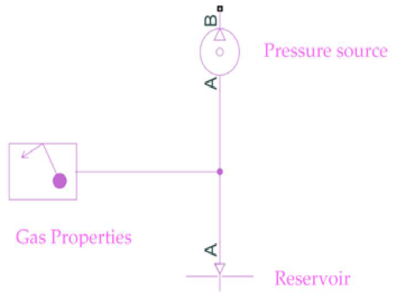
For simulating the gas behavior in SimScape, a supply unit, as shown in Figure 2, has been set up. The gas properties, together with the thermal conductivity and dynamic viscosity, which are used in modeling the gas transport behavior, are defined in the SimScape Gas properties block. The system’s reference temperature and pressure, which are taken as atmospheric temperature and pressure in this model, are defined by the SimScape Reservoir block, and the air compressor is modeled by a Pressure source block. The SimScape Pressure source block has two ports and is capable of maintaining a constant pressure difference between its ports. Therefore, by connecting the input port to the reservoir, a set pressure gas can be injected into the system.
The pipes in the system can be modeled using SimScape’s Pipe (G), thermal mass, convective heat transfer and temperature source blocks, as shown in Figure 3.
The parameters used in calculating the gas pressure drop and convective heat transfer between the gas flowing in the pipe and the pipe’s wall are set in the Pipe (G) block. The pressure drop at each end of the pipe is given as
where is the pipe’s cross-sectional area, and is the pressure losses due to viscous friction, . The notation is used to abbreviate the equations and can be replaced by or . This notation will be followed in the rest of this section. The pressure loss in a pipe depends on Reynolds numbers. The Reynolds number at each end of the pipe is equal to
where denotes the pipe’s diameter. If the calculated Reynolds number is less than 2000, the gas flow follows the laminar regime, and the pressure drop is equal to
For Reynolds numbers greater than 4000, the gas flow follows the turbulent flow regime, with a pressure drop of
denotes the pipe’s length and is the aggregate equivalent length of local resistances, which has been taken as 10% of the pipe’s length. The shape factor, , is considered as a constant number equal to 2.59, but the Darcy friction factor, , is a function of the Reynolds number and is equal to
where is the internal surface absolute roughness. For the Reynolds numbers between 2000 and 4000, a transition between laminar and turbulence regimes has been assumed.
The convective heat transfer between the gas flowing in the pipe and the pipe’s wall are modeled as
where and are the specific heat capacity and thermal conductivity calculated at the average temperature. is the Nusselt number, is the gas volume thermal conductivity, and and are the inlet and pipe internal wall temperatures, respectively. The value of the Nusselt number depends on the flow regime. For the laminar flow, the Nusselt number is taken as a constant, 3.66, and for turbulence flow is equal to
and are the Reynolds and Prandtl numbers, which are obtained at the average temperature.
The pipe properties for modeling the conduction heat transfer in the pipe’s wall can be adjusted in the thermal mass block, and the parameters for modeling the convective heat transfer between the pipe’s wall and the surrounding environment can be set in the convective heat transfer and temperature source blocks. The temperature source can maintain the atmospheric temperature regardless of the amount of heat flow into the system. The conduction heat transfer in the pipe’s wall can be mathematically modeled by
where , and are the pipe’s wall density, specific heat capacity, and temperature. Finally, the convective heat transfer between the pipe’s wall and the surrounding environment can be expressed as
where and are the surrounding air thermal conductivity and temperature.
The next component of the pneumatic actuator is the valve, which can be modeled as a set of restrictions capable of controlling the gas flow according to an input control signal. The restriction causes contraction of the gas at its input port, followed by the gas expansion at its output port, which results in a pressure drop across the ports. Considering the process as adiabatic, this pressure difference can be modeled as
where is the restriction’s cross-sectional area, and is the gas volume density at it. denotes the discharge coefficient, and is the ratio of the restriction cross-sectional area to the ports cross-sectional area. It is assumed that both ports have the same dimensions. As is seen from Equation (15), the pressure difference is proportional to the square of the gas flow rate, , which is typical in the turbulence regime. However, in the laminar regime, the pressure difference is linearly proportional to the gas flow rate, and thus can be approximated as
where and are the pressures of the inflow and outflow gases into the restriction, and is the laminar flow pressure ratio, which is taken as a constant, 0.999. The amount of pressure at the restriction is equal to
For the laminar regime, this can be approximated as
The local restriction (G) block has been used for modeling the valve in the SimScape environment. Each active state of the valve can be modeled by two local restriction blocks connecting ports P and T to ports A and B in Figure 1. The block allows modeling the valve leakage by defining a non-zero minimum restriction area, . Moreover, the valve spool displacement, , has been used to adjust the orifice area. The orifice cross-sectional area is linearly proportional to the spool displacement as
where is the maximum spool displacement causing the maximum cross-sectional area in the restriction, , and is the minimum value for the spool displacement. Figure 4 shows the model of the valve using SimScape components.
The complete model for the cylinder using SimScape blocks is depicted in Figure 5. The cylinder consists of two chambers, where each can be modeled using the translational mechanical converter (G) block in the SimScape to model the relation between the gas pressure inside a chamber and the applied mechanical force to the interface. Each cylinder chamber can be considered as an internal node, with a mass flow rate of
A heat flow rate of
where is the energy flow rate as a result of the gas transportation into/out of the chamber, and is due to the convective heat transfer between the gas in the chamber and the cylinder’s body. The partial derivative terms in Equations (20) and (21) can be obtained from Equations (3) and (5), respectively. Equations (11)–(14) are also applicable here to model the heat transfer between the gas in the chamber and the surrounding environment.
The gas volume in the chamber depends on the displacement of the moving interface, and is equal to
where denotes the dead volume, and and represent the interface cross-sectional area and displacement. The sign of the displacement value depends on the movement direction of the interface. The applied force to the interface can be expressed as
where is the atmospheric pressure. Therefore, the total force caused by the gas pressure in chambers 1 and 2, considering the forces’ directions, is equal to
Moreover, a translational hard stop block is used to restrict the cylinder interface movement within the length of the cylinder. The viscous friction coefficient for the piston movement can be modelled by a translational damper block. Two mass blocks are used for modelling the load and piston masses. The convective heat transfer, thermal mass, and temperature source blocks can model the heat transfer between the chamber gases and the surrounding environment. The motion equation for the load connected to the piston rod is equal to
where denotes the rod’s displacement, is the piston mass, and is the load mass, which causes the payload force of on the actuator. represents the viscous friction coefficient for the piston movement.
3. Controller Design
This section covers the procedure for designing an ILC controller for the considered pneumatic actuator covered in Section 2. The ILC method can generally be applied to repetitive processes. In such processes, every iteration starts and ends at the same conditions and lasts for a fixed period of time, . The state-space equation for a repetitive linear time-invariant system (with no feedthrough) can be represented as
denotes the trial number, and , and respectively represent the state variable vector, output, and input of the system at the iteration. are the state space system matrices. Suppose the system’s desired output for every iteration is , which makes the error at the iteration equal to
The idea of the ILC is to define a control law using previous trials’ information such that the error monotonically decreases in every new iteration until it reaches zero (). The control signal is calculated according to a recursive law as
If is designed in a way that , then the learning law is known as noncausal. Moreover, the control signal generated at the iteration can be calculated based on the information collected from all previous iterations. This method is called the high-order ILC (HOILC). However, a simplified law is preferred as long as it can attain the convergence with satisfactory speed.
The ILC algorithm can be presented in discrete-time, which is more suitable for being implemented by a microcontroller. For a sampling time of , where , the system can be considered as
, and . The system’s output can then be calculated as
where denotes the forward time-shift operator as . For a rational LTI system, can be expanded into
The error at the iteration is equal to
The ILC control law in the discrete-time domain can then be presented as
where represents any sample in the range of In such cases, it is common to implement the ILC method in the form of digital filters.
We begin our design by considering a general form for the ILC law as
To represent (34) in matrix format, let us consider sample sequences for the input, output and desired signals as
And , , and as matrices equal to
Therefore, (34) can be represented as
An ILC method is regarded to be asymptotically stable (AS) if
The converged control signal can be defined as , and in order for (37) to be AS,
where and is the eigenvalue of matrix .
Theorem 1.
The asymptotic error of the controlled system is equal to
whereis anidentity matrix.
Proof of Theorem 1.
Based on (32), and following (30) , which makes . Therefore, the asymptotic error, can be obtained as and by using (37) when
□
Theorem 2.
In order to have , , and should be selected as
Proof of Theorem 2.
From (40), for , we should have
□
Although by selecting matrices as (41), a zero asymptotic error can be achieved, and the transient error also needs to be analyzed to prevent having significant transient errors in the system response. The controlled system is called monotonically convergent if
where is the Euclidean norm, and is the convergence rate.
Theorem 3.
For the ILC law given in (34) we have,
wheredenotes the maximum singular value operator.
Proof of Theorem 3.
From (40), we have
and
Using values obtained in (41)
and
Therefore,
Considering that in ILC , we have where denotes an all one vector. Therefore,
Since for the matrices and given in (36) it can be proved that , we have
□
Using the results obtained from (39), (41), and (43), the ILC law given in (37) can achieve asymptotic stability as well as monotonic convergent and zero steady-state error when it is in the form of
However, further consideration has to be taken into account before using (44) to design a controller for the pneumatic actuator. First, the considered pneumatic actuator is a nonlinear system with the state space equation of
We assume that and are global Lipschitz continuous (GLC) functions. Therefore,
By taking into account that the considered pneumatic system is asymptotically stable and for a sampling time of , where , the system can be considered as
where and . This follows the Lyapunov stability analysis, where it is assumed that for a physically stable system all the linear terms are in and and higher-order terms are in and , in the sense that when gets small, and get small faster. This means that the nonlinearities’ effects in the system’s dynamic would eventually vanish, and that the system has a dominating linear characteristic at its steady-state condition. The remaining nonlinearities is as a result of input effect, , which can be denoted as . Using (47), the system’s output can be presented as
where term is as a result of the nonlinearities’ residue in the model. By applying the proposed ILC law given in (37), we have
In order to make sure that the ILC method is AS, an additional term has been added to the ILC law as
where . The existence of is guaranteed as and are assumed to be GLC functions. As the nonlinearities in the system can be controlled (removed) by adding the proportional control term, , the rest of the system can be considered linear, and (39), (41), and (43) will be held.
The ILC, in theory, is effective for repetitive processes. However, we would like to expand the ILC application to control the pneumatic system responding to non-repetitive inputs and disturbances. For this purpose, the proof given for Theorem 3 has to be revisited. As part of this proof, we had
However, as the process is not repetitive, we cannot consider . Instead, we should select the value as its maximum, since this choice can help the condition to be asymptotically held as . Therefore, the ILC law for controlling the pneumatic actuator can be summarized as:
4. Results and Discussion
Table 1 presents the parameters’ values used in simulating the piston-cylinder pneumatic actuator.
The effect of applied voltage on the valve’s cross-sectional area, where the valve supplies port B for the negative voltage values and connects the supply port P to port A for the positive values, is shown in Figure 6. As is seen, a dead-band behavior appears in the vicinity of 0 V. This follows the pattern of the same in the physical actuator studied in [44], shown in Figure 6 of this reference.
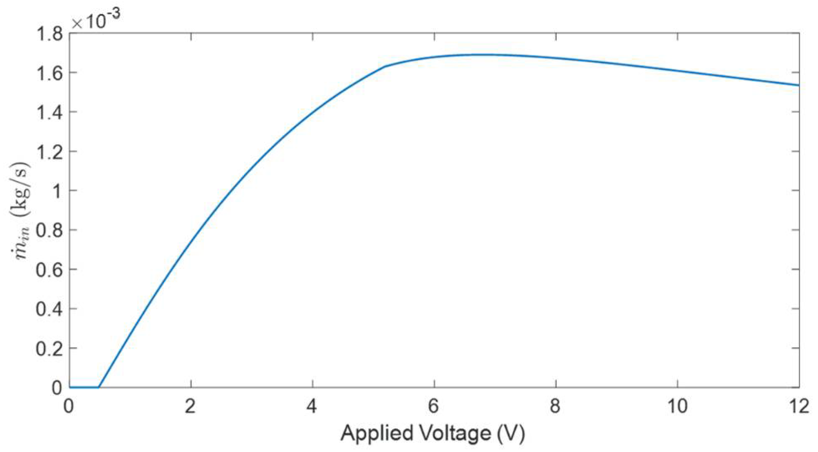
The gas flow rate, , in the valve with respect to the applied voltage values is presented in Figure 7. As a result of leakage, the gas flow rate for the applied voltage less than ~0.5 V remains at zero. By applying more voltage, the gas flow rate increases by following a laminar regime until it reaches a point that the flow rate enters into a turbulence regime, in which a decrease in the flow rate slope can be observed. This follows the pattern of the same in the physical actuator studied in [44] shown in the Figure 7 of this reference.
We then apply an input voltage to the valve and measure the rod’s displacement. This is depicted in Figure 8. The input signal is selected in such a way as to take the valve’s spool to its extreme positions. An applied 12 V signal charges chamber 1 and allows gas to be exhausted from chamber 2, which causes the rod to extend to its maximum displacement, 0.2 m. The signal has been applied long enough so that the system can be settled. The valve is then moved to its neutral state by applying 0 V, and as is shown, the rod’s displacement remains unchanged. By applying −12 V to the valve, the gas in chamber 1 exhausts, and chamber 2 fills with gas, moving the piston inward until it reaches zero. Again, a 0 V signal has been applied to move the valve to its neutral state, where holding the rod’s position unchanged. The response transition time is around 2 s.
The frequency response of the system has also been studied. As was discussed, the air is compressible and has a low damping characteristic, which causes a nonlinear response and increases the pneumatic system’s dynamic order. Moreover, before the system can apply any force to a load, the pipes and cylinders have to be filled with air. This results in further nonlinearities in the form of dead-band and transmission attenuations. Moreover, a pneumatic system is affected by frictional forces caused by the mechanical parts’ movements. All these uncertainties and nonlinearities make linearizing a pneumatic system a complicated practice that generates inaccurate results. Therefore, a system identification approach has been implemented to estimate the frequency response of the pneumatic actuator. In this approach, a set of sinusoidal signals with different frequencies are applied to the system and the piston’s rod displacement is measured. The collected results are then used to draw the system’s bode plot. The estimated bode plot for the pneumatic actuator obtained by applying sinusoidal voltage signals in the range of 0.5 to 100 Hz is given in Figure 9, showing around 1.6 rad/s frequency bandwidth for the considered pneumatic actuator.
According to [45], servo pneumatic actuators in approximately 70% of industrial applications should move 1–10 kg payloads with ±2 to ±0.02 mm precision. Therefore, in this paper, we consider the same criteria in studying the performance of the designed controllers. One major advantage of ILC is that it does not need accurate knowledge of the system model, and instead, it can learn from the system’s historical input and output. However, some degree of estimation can help to obtain a better design with a faster convergence. For this purpose, the estimated bode plot, given in Figure 9, will be used. As is seen, the system is a lowpass with the bandwidth of 1.6 rad/s. Therefore, we use
to estimate the linear part of the system. Since the system’s bandwidth is 1.6 rad/s, it can be assumed that the system does not have much of fluctuations over a period of one second. Therefore, by taking , we can consider that the system would be seen as a repetitive process from the controller’s perspective. The for the system given by (53) based on is equal to
and
should be selected such that and . Theoretically, will perfectly satisfy both conditions. However, as
this design would take the system into saturation due to its high gain value of . Considering the maximum rod’s displacement as 0.2 m and the maximum input voltage as 12 V, the maximum gain value should be limited to Another observation from (56) is that the maximum number of non-zero elements in each column is two, which means that regardless of the selected value for , only two consecutive samples are used in the control law. As a result, would be sufficient for implementing the ILC to control this pneumatic actuator. Therefore, we consider as a lower triangular matrix and calculate its arrays’ values.
Although from the theoretical perspective, a larger value of improves the AS condition of the ILC method, from the practical aspect, it should be limited to 60 to prevent the system from saturation. Figure 10 shows the relation between and to avoid saturation. From a repetitive process perspective, the best value would be to minimize the transient error as is given by (43). However, the inputs to the considered pneumatic system are not repetitive, and following (52), the values in (57) are selected as , which makes and , satisfying the conditions in (52). The value for should be in the range of to satisfy the AS condition of the ILC method, which we adjusted to 0.25 in this design. However, choosing the optimal value for requires the system’s knowledge, which is not available.
Based on the above discussions, the designed ILC method for the pneumatic actuator system is implemented as
We further used the obtained frequency response of the system, given in Figure 9, to design a PID controller in order to compare its performance to that of the proposed ILC method. The frequency domain techniques, namely the Nichols chart and Inverse Nichols chart, have been used to achieve the required performance in reference tracking and disturbance rejection. To obtain the precision of ±0.002 m, the tracking boundaries are designed to be in the range of
and the sensitivity bound is designed to be less than 3 dB for the lower frequencies () and less than 6 dB for all frequencies. The obtained PID controller is calculated as
Moreover, two recently proposed intelligent model-free control approaches have been selected to compare the performance of the designed ILC method with theirs. The first approach, proposed in [46], uses type-2 Takagi–Sugeno (T-S) fuzzy systems with the memory state feedback control. The controller is expressed using the state variable as
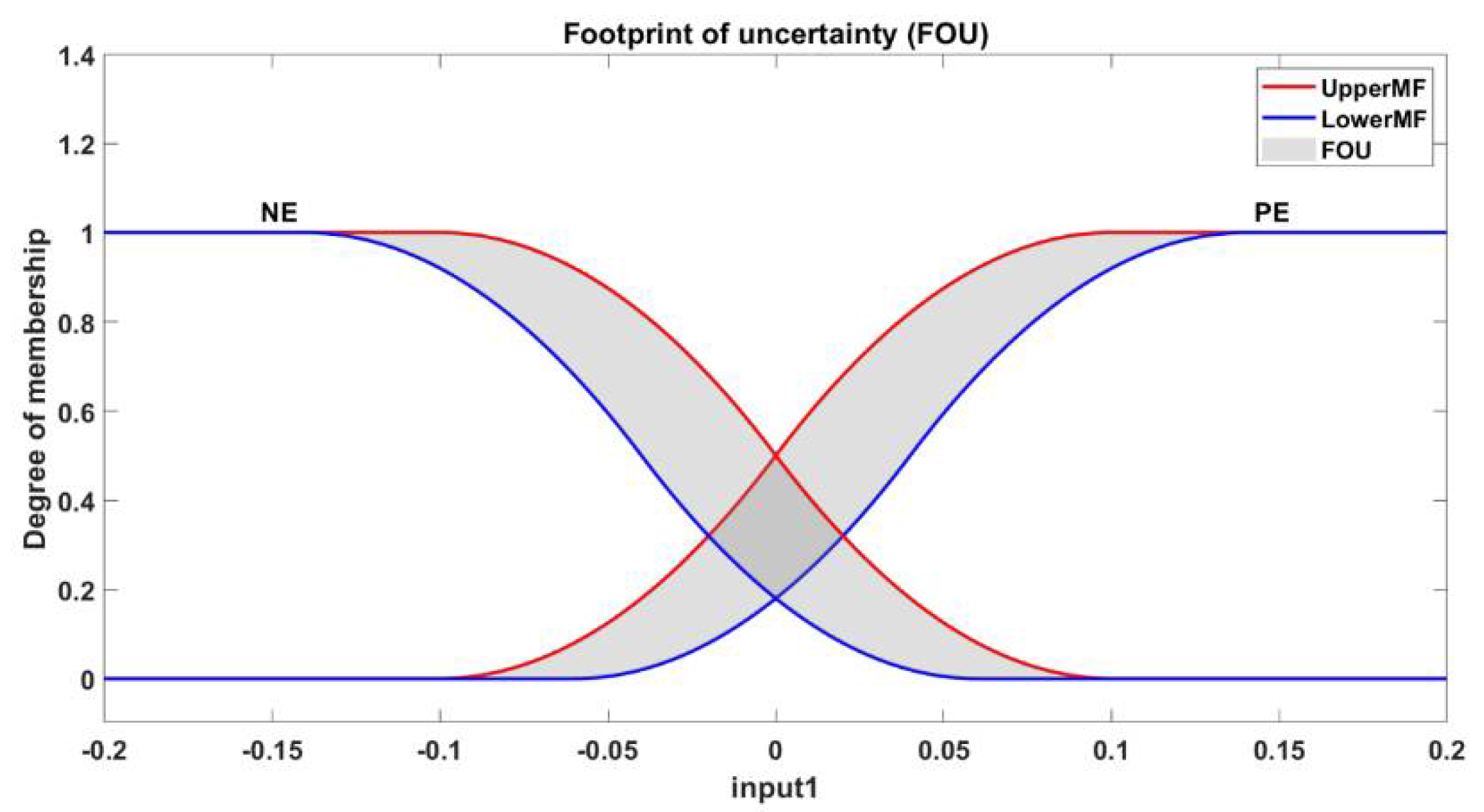
where denotes the interval type-2 (IT2) fuzzy set of the premise variable, , and and are the number of fuzzy IF-THEN rules and fuzzy sets of controller, respectively. are nonlinear weight coefficient functions that are calculated based on upper and lower membership functions. The footprint of uncertainty (FOU) for the employed T-S fuzzy system is given in Figure 11. Two fuzzy rules are defined taking the system error as the state variable and the coefficients are selected according to a procedure explained in the reference as and . The feedback control gains are then calculated as and .
In the other approach proposed in [47], a type-1 T–S fuzzy observer is used to develop a piecewise control strategy for dealing with the nonlinear terms in the system. The membership functions employed for constructing the observer is depicted in Figure 12. The controller gain is calculated as [5.37, −5.37].
The performance of the controllers in tracking a reference signal under a constant load of 10 kg is shown in Figure 13. As is seen, the designed ILC is capable of tracking a non-repetitive signal. Next, we compare the performance of the ILC with the other controllers, which is given in Table 2. It can be seen that the ILC demonstrates a faster response, however, it demonstrates overshoots in the transient response. The maximum overshoot percentage happens during the forward motion when the actuator moves from the resting to reach 0.1 m, which equals 13.5%. This can be considered as the major drawback of the ILC, which is caused by the way that ILC calculates the control signal. The ILC only modifies the control signal according to predefined control law and based on the historical input and output. Therefore, a sudden change in the input signal will cause overshoot in the control signal. However, in a well-designed ILC that holds monotonic convergent, the gap between the input and output is reduced after sufficient iterations. The ILC can obtain ±0.002 m precision (2% settling time) in 0.52 s compared to 0.46 s for the PID and 0.35 s for the IT2 T_S fuzzy controller. The controller based on T-S fuzzy observer could not achieve the required precision. The difference between the reference and output of the system controlled by each of these controllers is shown in Figure 14, and the summation of the square of the error () is given in Table 2. The ILC demonstrates superior performance than other controllers in terms of both speed (rise time) and tracking accuracy.
Next, we compare the performance of the controllers in overcoming the payload uncertainty, as is shown in Figure 15. The top plot in this figure shows the payload variation applied to the piston while the reference signal remains constant at 0.1 m. As is seen, the ILC-controlled system can maintain the required precession (±0.002 m) regardless of changes in the load. However, this cannot be adequately achieved with the other controllers. The plot of the disturbance rejection error is given in Figure 16. The summation of the square of the error for the controllers is given in Table 3. Again, the ILC shows a better performance than the other controllers in overcoming the uncertainties.
5. Conclusions
This paper suggested an effective model-free control scheme to overcome the nonlinearities and uncertainties resulting from air characteristics, pressure loss, leakage, and load variations in a pneumatic system. In the majority of the control algorithms used in controlling the position of a pneumatic actuator, the model of the system has to be achieved prior to the design of the controller. However, due to the physical behavior of the gases, modelling a pneumatic system is usually done based on many assumptions that might result in an inaccurate model during system operation. As a result, such controllers may not achieve the required performance. Moreover, intelligence-based control algorithms cannot easily be implemented in real-time applications due to their extensive calculation requirements. This leads to a need for developing real-time control systems capable of controlling pneumatic systems without needing to obtain the mathematical model of the system. An ILC algorithm uses information from previous repetitions to learn about the system’s dynamics for generating a more suitable control signal. ILC algorithms are particularly useful in real-time control systems, given their relatively quick response to changes in the input signal. However, their application is only limited to repetitive processes, where the same control action should be performed repeatedly. In this paper, the application of the ILC algorithm has been expanded for controlling nonlinear, non-repetitive systems. Moreover, a pneumatic cylinder-piston actuator has been simulated using MATLAB SimScape blocks and the simulation results showed that the model can successfully demonstrate the behavior of a pneumatic system. The procedure for designing an ILC controller without needing any information on the system model and by only using the system’s input and output measurements has been covered. The simulation results showed that the designed ILC controller is capable of tracking a non-repetitive reference signal and can overcome the internal and payload uncertainties with the precision of 0.002 m. Therefore, the ILC can be considered as an approach for controlling the pneumatic actuators, which is challenging to obtain their mathematical modeling.
Author Contributions
Conceptualization, J.R. and F.G.; methodology, J.R. and F.G.; software, J.R. and F.G.; validation, J.R. and F.G.; formal analysis, J.R. and F.G.; investigation, J.R. and F.G.; resources, F.G.; data curation, J.R. and F.G.; writing—original draft preparation, J.R. and F.G.; writing—review and editing, F.G.; visualization, J.R.; supervision, F.G.; project administration, F.G.; funding acquisition, F.G. All authors have read and agreed to the published version of the manuscript.
Funding
This research received no external funding.
Institutional Review Board Statement
Not applicable.
Informed Consent Statement
Not applicable.
Data Availability Statement
Not applicable.
Conflicts of Interest
The authors declare no conflict of interest.
References
- Krause, J.; Bhounsule, P. A 3D Printed Linear Pneumatic Actuator for Position, Force and Impedance Control. Actuators 2018, 7, 24. [Google Scholar] [CrossRef] [Green Version]
- Rosli, R.; Mailah, M.; Priyandoko, G. Active suspension system for passenger vehicle using active force control with iterative learning algorithm. WSEAS Trans. Syst. Control 2014, 9, 120–129. [Google Scholar]
- Bu, F.; Tan, H.-S. Pneumatic brake control for precision stopping of heavy-duty vehicles. IEEE Trans. Control. Syst. Technol. 2006, 15, 53–64. [Google Scholar] [CrossRef] [Green Version]
- Kadam, S.; Gaikwad, V.; Bhavsar, H.; Kulkarni, S. Electro-Pneumatic Lift and Carry Conveying System. Int. J. Sci. Technol. Eng. 2016, 2, 904–907. [Google Scholar]
- Davis, S. Pneumatic Actuators. Actuators 2018, 7, 62. [Google Scholar] [CrossRef] [Green Version]
- Nguyen, H.T.; Trinh, V.C.; Le, T.D. An Adaptive Fast Terminal Sliding Mode Controller of Exercise-Assisted Robotic Arm for Elbow Joint Rehabilitation Featuring Pneumatic Artificial Muscle Actuator. Actuators 2020, 9, 118. [Google Scholar] [CrossRef]
- Walker, J.; Zidek, T.; Harbel, C.; Yoon, S.; Strickland, F.S.; Kumar, S.; Shin, M. Soft Robotics: A Review of Recent Developments of Pneumatic Soft Actuators. Actuators 2020, 9, 3. [Google Scholar] [CrossRef] [Green Version]
- Su, H.; Hou, X.; Zhang, X.; Qi, W.; Cai, S.; Xiong, X.; Guo, J. Pneumatic Soft Robots: Challenges and Benefits. Actuators 2022, 11, 92. [Google Scholar] [CrossRef]
- Bone, G.M.; Xue, M.; Flett, J. Position control of hybrid pneumatic–electric actuators using discrete-valued model-predictive control. Mechatronics 2015, 25, 1–10. [Google Scholar] [CrossRef]
- Hamiti, K.; Voda-Besancon, A.; Roux-Buisson, H. Position control of a pneumatic actuator under the influence of stiction. Control Eng. Pract. 1996, 4, 1079–1088. [Google Scholar] [CrossRef]
- Li, Y.; Zhou, W.; Wu, J.; Hu, G. A Dynamic Modeling Method for the Bi-Directional Pneumatic Actuator Using Dynamic Equilibrium Equation. Actuators 2022, 11, 7. [Google Scholar] [CrossRef]
- Rouzbeh, B.; Bone, G.M. Optimal Force Allocation and Position Control of Hybrid Pneumatic–Electric Linear Actuators. Actuators 2020, 9, 86. [Google Scholar] [CrossRef]
- Van Varseveld, R.B.; Bone, G.M. Accurate position control of a pneumatic actuator using on/off solenoid valves. IEEE/ASME Trans. Mechatron. 1997, 2, 195–204. [Google Scholar] [CrossRef]
- Saleem, A.; Wong, C.-B.; Pu, J.; Moore, P.R. Mixed-reality environment for frictional parameters identification in servo-pneumatic system. Simul. Model. Pract. Theory 2009, 17, 1575–1586. [Google Scholar] [CrossRef]
- Wang, J.; Pu, J.; Moore, P. A practical control strategy for servo-pneumatic actuator systems. Control. Eng. Pract. 1999, 7, 1483–1488. [Google Scholar] [CrossRef]
- Sudani, M.; Deng, M.; Wakimoto, S. Modelling and Operator-Based Nonlinear Control for a Miniature Pneumatic Bending Rubber Actuator Considering Bellows. Actuators 2018, 7, 26. [Google Scholar] [CrossRef] [Green Version]
- Wang, J.; Kotta, Ü.; Ke, J. Tracking Control of Nonlinear Pneumatic Actuator Systems Using Static State Feedback Linearization of the Input-Output Map. Proc. Est. Acad. Sci. Phys. Math. 2007, 56, 47–66. [Google Scholar]
- Karim, K.; Pascal, B.; Louis, A. Force control loop affected by bounded uncertainties and unbounded inputs for pneumatic actuator systems, ASME. J. Dyn. Syst. Meas. Control 2008, 130, 011007. [Google Scholar]
- Khayati, K.; Bigras, P.; Dessaint, L.-A. A robust feedback linearization force control of a pneumatic actuator. In Proceedings of the 2004 IEEE International Conference on Systems, Man and Cybernetics (IEEE Cat. No. 04CH37583), The Hague, The Netherlands, 10–13 October 2004; IEEE: Piscataway, NJ, USA, 2004; pp. 6113–6119. [Google Scholar]
- Karpenko, M.; Sepehri, N. QFT design of a PI controller with dynamic pressure feedback for positioning a pneumatic actuator. In Proceedings of the 2004 American Control Conference, Boston, MA, USA, 30 June–2 July 2004; IEEE: Piscataway, NJ, USA, 2004; pp. 5084–5089. [Google Scholar]
- Karpenko, M.; Sepehri, N. QFT synthesis of a position controller for a pneumatic actuator in the presence of worst-case persistent disturbances. In Proceedings of the 2006 American Control Conference, Minneapolis, MN, USA, 14–16 June 2006; IEEE: Piscataway, NJ, USA, 2006; p. 6. [Google Scholar]
- Lin, Z.; Xie, Q.; Qian, Q.; Zhang, T.; Zhang, J.; Zhuang, J.; Wang, W. A Real-Time Realization Method for the Pneumatic Positioning System of the Industrial Automated Production Line Using Low-Cost On–Off Valves. Actuators 2021, 10, 260. [Google Scholar] [CrossRef]
- Lin, C.-J.; Sie, T.-Y.; Chu, W.-L.; Yau, H.-T.; Ding, C.-H. Tracking Control of Pneumatic Artificial Muscle-Activated Robot Arm Based on Sliding-Mode Control. Actuators 2021, 10, 66. [Google Scholar] [CrossRef]
- Hidalgo, M.C.; Garcia, C. Friction compensation in control valves: Nonlinear control and usual approaches. Control Eng. Pract. 2017, 58, 42–53. [Google Scholar] [CrossRef]
- Tsai, Y.-C.; Huang, A.-C. FAT-based adaptive control for pneumatic servo systems with mismatched uncertainties. Mech. Syst. Signal Process. 2008, 22, 1263–1273. [Google Scholar] [CrossRef]
- Shtessel, Y.; Plestan, F.; Taleb, M. Lyapunov design of adaptive super-twisting controller applied to a pneumatic actuator. IFAC Proc. Vol. 2011, 44, 3051–3056. [Google Scholar] [CrossRef] [Green Version]
- Zhu, Y.; Barth, E.J. Accurate sub-millimeter servo-pneumatic tracking using model reference adaptive control (MRAC). Int. J. Fluid Power 2010, 11, 43–55. [Google Scholar] [CrossRef]
- Farag, M.; Azlan, N.Z. Adaptive Backstepping Position Control of Pneumatic Anthropomorphic Robotic Hand. Procedia Comput. Sci. 2015, 76, 161–167. [Google Scholar] [CrossRef] [Green Version]
- Yamazaki, M.; Yasunobu, S. An intelligent control for state-dependent nonlinear actuator and its application to pneumatic servo system. In Proceedings of the SICE Annual Conference 2007, Takamatsu, Japan, 17–20 September 2007; IEEE: Piscataway, NJ, USA, 2007; pp. 2194–2199. [Google Scholar]
- Najjari, B.; Barakati, S.M.; Mohammadi, A.; Futohi, M.J.; Bostanian, M. Position control of an electro-pneumatic system based on PWM technique and FLC. ISA Trans. 2014, 53, 647–657. [Google Scholar] [CrossRef]
- dos Santos, M.P.S.; Ferreira, J. Novel intelligent real-time position tracking system using FPGA and fuzzy logic. ISA Trans. 2014, 53, 402–414. [Google Scholar] [CrossRef]
- Yao, B.; Zhou, Z.; Liu, Q.; Ai, Q. Empirical modeling and position control of single pneumatic artificial muscle. J. Control. Eng. Appl. Inform. 2016, 18, 86–94. [Google Scholar]
- Živčák, J.; Kelemen, M.; Virgala, I.; Marcinko, P.; Tuleja, P.; Sukop, M.; Liguš, J.; Ligušová, J. An Adaptive Neuro-Fuzzy Control of Pneumatic Mechanical Ventilator. Actuators 2021, 10, 51. [Google Scholar] [CrossRef]
- Li, Y.; Cao, Y.; Jia, F. A Neural Network Based Dynamic Control Method for Soft Pneumatic Actuator with Symmetrical Chambers. Actuators 2021, 10, 112. [Google Scholar] [CrossRef]
- Kaitwanidvilai, S.; Parnichkun, M. Force control in a pneumatic system using hybrid adaptive neuro-fuzzy model reference control. Mechatronics 2005, 15, 23–41. [Google Scholar] [CrossRef]
- Alexandru, S.; Gheorghe, P.; Bogdan, C. Aspects regarding the neuroadaptive control structure properties application to the nonlinear pneumatic servo system benchmark, Electrotechnics. Electron. Autom. Control. Inform. 2006, 29, 82–86. [Google Scholar]
- Moore, K.L. Iterative Learning Control for Deterministic Systems; Springer: Berlin/Heidelberg, Germany, 2012. [Google Scholar]
- Hunt, K.J.; Sbarbaro, D.; Żbikowski, R.; Gawthrop, P.J. Neural networks for control systems—A survey. Automatica 1992, 28, 1083–1112. [Google Scholar] [CrossRef]
- Chen, C.-K.; Hwang, J. Iterative learning control for position tracking of a pneumatic actuated XY table. In Proceedings of the 2004 IEEE International Conference on Control Applications, Taipei, Taiwan, 2–4 September 2004; IEEE: Piscataway, NJ, USA, 2004; pp. 388–393. [Google Scholar]
- Yu, S.; Bai, J.; Xiong, S.; Han, R. A new iterative learning controller for electro-pneumatic servo system. In Proceedings of the 2008 Eighth International Conference on Intelligent Systems Design and Applications, Kaohsuing, Taiwan, 26–28 November 2008; IEEE: Piscataway, NJ, USA, 2008; pp. 101–105. [Google Scholar]
- Qian, K.; Li, Z.; Asker, A.; Zhang, Z.; Xie, S. Robust Iterative Learning Control for Pneumatic Muscle with State Constraint and Model Uncertainty. In Proceedings of the 2021 IEEE International Conference on Robotics and Automation (ICRA), Xi’an, China, 30 May–5 June 2021; IEEE: Piscataway, NJ, USA, 2021; pp. 5980–5987. [Google Scholar]
- Ai, Q.; Ke, D.; Zuo, J.; Meng, W.; Liu, Q.; Zhang, Z.; Xie, S.Q. High-order model-free adaptive iterative learning control of pneumatic artificial muscle with enhanced convergence. IEEE Trans. Ind. Electron. 2019, 67, 9548–9559. [Google Scholar] [CrossRef]
- Rwafa, J.; Ghayoor, F. Implementation Of Iterative Learning Control on a Pneumatic Control Valve. In Proceedings of the 2019 International Multidisciplinary Information Technology and Engineering Conference (IMITEC), Vanderbijlpark, South Africa, 21–22 November 2019; IEEE: Piscataway, NJ, USA, 2019; pp. 1–5. [Google Scholar]
- Richer, E.; Hurmuzlu, Y. A high performance pneumatic force actuator system: Part I—Nonlinear mathematical model. J. Dyn. Syst. Meas. Control 2000, 122, 416–425. [Google Scholar] [CrossRef]
- Krivts, I.L.; Krejnin, G.V. Pneumatic Actuating Systems for Automatic Equipment: Structure and Design; CRC Press: Boca Raton, FL, USA, 2016. [Google Scholar]
- Kavikumar, R.; Sakthivel, R.; Kwon, O.; Kaviarasan, B. Faulty actuator-based control synthesis for interval type-2 fuzzy systems via memory state feedback approach. Int. J. Syst. Sci. 2020, 51, 2958–2981. [Google Scholar] [CrossRef]
- Song, X.; Wang, M.; Ahn, C.K.; Song, S. Finite-time fuzzy bounded control for semilinear PDE systems with quantized measurements and markov jump actuator failures. IEEE Trans. Cybern. 2021, 52, 5732–5743. [Google Scholar] [CrossRef]
Figure 1.
The considered pneumatic actuator.

Figure 2.
The SimScape model of the supply unit.

Figure 3.
The SimScape model of the pipe.

Figure 4.
The SimScape model of the valve.

Figure 5.
The SimScape model of the cylinder.

Figure 6.
Changes in the input valve cross-sectional area with the applied voltage.

Figure 7.
Mass flow rate in the valve versus the applied voltage.

Figure 8.
Effect of the valve’s input voltage on the rod’s displacement.

Figure 9.
The pneumatic system estimated frequency response.

Figure 10.
The effect of learning function value on the

Figure 11.
Footprint of uncertainty.

Figure 12.
Membership functions.

Figure 13.
The comparison of the controllers’ performance in tracking a reference signal.

Figure 14.
The comparison of controllers’ performance with respect to the tracking error.

Figure 15.
The comparison between the controllers’ performance in the disturbance rejection.

Figure 16.
The comparison of the controllers’ performance with respect to the disturbance rejection error.
Figure 16.
The comparison of the controllers’ performance with respect to the disturbance rejection error.


Table 1.
Parameters values used in simulation.
| Parameter Name | Parameter Value | |
|---|---|---|
| Gas Properties | Supply pressure (Ps) | 7 × 10⁵ (Pa) |
| Supply temperature (Ts) | 293.15 (K) | |
| Gas constant (R) | 287 (J/(kg·K)) | |
| Specific enthalpy (h) | 293.6 (kJ/kg) | |
| Compressibility factor (z) | 0.999 | |
| Specific heat capacity (Cp) | 1.01 (kJ/(kg·K)) | |
| Thermal conductivity () | 25.7 (mW/(K.m)) | |
| Dynamic viscosity () | 18.2 (Pa·s) | |
| Specific heat ratio () | 1.4 | |
| Reference temperature (T0) | 293.15 (K) | |
| Atmosphere pressure (Patm) | 1 × 10⁵ (Pa) | |
| Valve Properties | Discharge coefficient (Cd) | 0.82 |
| Max orifice area (Amax) | 4 × 10⁻⁶ (m2) | |
| Leakage area (Aleakage) | 1 × 10⁻¹⁰ (m2) | |
| Displacement for leakage area (xleakage) | 2 × 10⁻⁴ (m) | |
| Displacement limit (xmax) | 5 × 10⁻³ (m) | |
| Input voltage range | [–12, 12] (V) | |
| Pipe Properties | Length (Lt) | 1 (m) |
| Pipe cross-sectional area (At) | 5 × 10⁻⁶ (m) | |
| Internal surface absolute roughness () | 15 × 10−6 (m) | |
| Pipe wall density () | 1500 (kg/m3) | |
| Pipe wall specific heat capacity (Ct) | 1250 (J/(kg·K)) | |
| Wall-air heat transfer coefficient () | 20 (W/(m2·K)) | |
| Cylinder Properties | Initial interface displacement (Linit) | 0 (m) |
| Max piston stroke (Lp) | 0.2 (m) | |
| Interface cross-sectional area (Ap) | 0.002 (m2) | |
| Dead volume (Vd) | 4 × 10⁻⁵ (m3) | |
| Gas-wall heat transfer coefficient () | 100 (W/(m2·K)) | |
| Actuator wall specific heat (CCylinder) | 870 (J/(kg·K)) | |
| Actuator mass (MC) | 3 (kg) | |
| Piston mass (MP) | 1 (kg) | |
| Hard stop stiffness (khs) | 1 × 10⁷ (N/m) | |
| Hard stop damping () | 1500 (N/(m·s)) | |
| Mechanical damping () | 200 (N/(m·s)) |
Table 2.
Comparison between the controllers’ performance in tracking a signal.
| Controller | Rise Time (s) | Overshoot | Settling Time | Error |
|---|---|---|---|---|
| ILC | 0.2 | 13.5% | 0.52 | 0.0044 |
| PID | 0.26 | 0 | 0.46 | 0.0049 |
| IT2 T-S fuzzy | 0.24 | 0 | 0.35 | 0.0048 |
| T-S fuzzy obs. | 0.38 | 0 | -- | 0.0081 |
Table 3.
Comparison between the controllers’ performance in disturbance rejection.
| Controller | Error |
|---|---|
| ILC | |
| PID | |
| IT2 T-S fuzzy | |
| T-S fuzzy obs. |
Publisher’s Note: MDPI stays neutral with regard to jurisdictional claims in published maps and institutional affiliations. |
© 2022 by the authors. Licensee MDPI, Basel, Switzerland. This article is an open access article distributed under the terms and conditions of the Creative Commons Attribution (CC BY) license (https://creativecommons.org/licenses/by/4.0/).
Share and Cite
MDPI and ACS Style
Rwafa, J.; Ghayoor, F. Implementation of Iterative Learning Control on a Pneumatic Actuator. Actuators 2022, 11, 240. https://doi.org/10.3390/act11080240
AMA Style
Rwafa J, Ghayoor F. Implementation of Iterative Learning Control on a Pneumatic Actuator. Actuators. 2022; 11(8):240. https://doi.org/10.3390/act11080240
Chicago/Turabian StyleRwafa, James, and Farzad Ghayoor. 2022. "Implementation of Iterative Learning Control on a Pneumatic Actuator" Actuators 11, no. 8: 240. https://doi.org/10.3390/act11080240
Note that from the first issue of 2016, this journal uses article numbers instead of page numbers. See further details here.