
Using Feature Extraction to Perform Equipment Health Monitoring on Ship-Radiated Noise

Department of Electrical and Computer Engineering, Royal Military College of Canada, Station Forces, Kingston, ON K7K 7B4, Canada
*
Author to whom correspondence should be addressed.
†
These authors contributed equally to this work.
Acoustics 2023, 5(4), 1180-1193; https://doi.org/10.3390/acoustics5040067
Submission received: 14 September 2023
/
Revised: 29 November 2023
/
Accepted: 12 December 2023
/
Published: 18 December 2023
(This article belongs to the Special Issue Vibration and Noise)
Abstract
:The current state of the art in hydroacoustics research employs a variety of feature extraction techniques with the goal of accurately classifying a ship based on its radiated noise. These techniques are capable of accuracy in excess of 95%. A question arises as to whether similar techniques could be applied to a known vessel to identify and monitor individual systems from the ship’s noise. In this paper, the fast orthogonal search algorithm is used as a basis for a feature extraction and classification algorithm. This algorithm is applied to real recordings of ship-radiated noise and is shown to be capable of identifying the running status of a subset of the ship’s systems, providing a proof of concept for the detection and monitoring of a ship’s systems based solely on the ships hydroacoustic noise.
1. Introduction
One of the primary motivations driving research in the area of ship-radiated noise has been in improving the ability to detect ships [1,2]. Lately, however, a wealth of data processing techniques have arisen and allowed research to expand beyond simply detecting a vessel and instead seeking to classify a vessel. Several researchers have posed the question whether, based solely on the acoustic noise generated by a ship, the type of ship or even the specific ship can be identified reliably [3,4,5]. Techniques for this classification vary, but can generally be described by a few broad approaches. One approach is to directly analyze the acoustic data in the time or frequency domain and attempt to fashion an approximate representation of the ship’s radiated signal with which to compare future samples [5,6]. Alternately, the acoustic data can be decomposed into intrinsic mode functions (IMFs), and the IMFs can be analyzed for characteristic features, such as the energy difference between IMFs [5]. Finally, a signal can be decomposed into IMFs and a single IMF selected and analyzed for characteristic features, such as the energy entropy within the IMF or the IMF centre frequency [7,8]. These approaches allow for a variety of signal processing algorithms to be employed and have been shown to be highly effective in the identification of ships from a small sample of candidates, with some techniques exceeding 95% accuracy [3]. Given the high accuracy of identifying ships based on their radiated noise, the question arises of whether, if the ship was known, these analysis techniques could allow the detection and monitoring of specific systems within the ship.
Machinery generates noise and vibration that, if monitored, can vary as machinery degrades or develops defects. Techniques that harness the relationships between equipment health and their noise or vibration, which are part of a broader set of techniques that monitor machinery health known as equipment health monitoring (EHM), can analyze rotating or reciprocating equipment in order to detect potential mechanical defects. Shipboard mechanical noise is generated by rotating and reciprocating components, cavitation, and friction between components [9]. When spectrally analyzed, this noise presents as strong line spectra and weak continuous spectrum noise. For main propulsion machinery, the frequency and amplitude of the noise is heavily dependent on the ship’s speed. However, for auxiliary machinery, the frequency and magnitude of the noise tend to be independent of the ship’s speed, and generally stable in time [9].
The fast orthogonal search (FOS) algorithm is a signal estimation and spectral analysis algorithm. It has been shown under experimental conditions to provide superior frequency resolution and be more capable of identifying line component spectra than the fast Fourier transform (FFT) [10,11]. This ability has led to research interest in the algorithm as a tool for EHM. One such application was the development of a technique for structural health monitoring (SHM) based on the FOS algorithm [12]. This would be useful in shipboard applications as a method to monitor hull stress and fatigue. Additionally, the FOS algorithm has been used as a basis for health monitoring tools for induction motors, being shown to diagnose broken rotor bars in a motor with greater accuracy and smaller sample times than a similar technique using the FFT [13]. The use of FOS as a tool for diagnosing induction machine faults is especially interesting to shipboard EHM, as recent advances in induction motor technology have led induction machines to be the ideal choice for all-electric drive ships [14]. Given that the FOS algorithm is already an area of research for EHM and it has been shown to provide superior spectral analysis and noise resistance than other frequency analysis tools, it is an ideal candidate for feature extraction from ship radiated noise (SRN) in order to identify and monitor ships’ systems.
The FOS algorithm generates an approximation of an input signal by creating a weighted summation of a select subset of predetermined candidate functions. The candidate functions are selected for inclusion in the functional expansion generated by the algorithm via statistical correlation between the candidate function and the input signal. The function with the greatest correlation to the input signal, which represents the most possible fitted energy, is selected as the first term in the functional expansion. Subsequent terms further reduce the mean square error (MSE) between the estimation and the input signal. This is continued until a stopping condition for the algorithm has been satisfied. These conditions can vary based on the specific implementation of the algorithm and can include a minimum amount of the input signal’s energy having been fit, the inability of the algorithm to reduce the MSE between the functional expansion and the input signal with any remaining candidate functions, or simply a desired number of candidate functions being fit. A full explanation of the FOS algorithm can be found in Appendix A.
In this paper, the FOS algorithm is applied to samples of real-world SRN, acquired through recordings of Patrol Craft, Training (PCT) Moose during hydroacoustic range trials. FOS is used to preform spectral analysis of training data in order to identify features of specific systems onboard PCT Moose. It is then used to create classifiers based on these features, which are tested for their ability to accurately predict the running status of these systems. The success of these classifiers and their improved accuracy over a similar classifier based on the FFT demonstrate the feasibility of using acoustic processing techniques to identify discrete components from a ship’s noise and provide an argument for continued research in this application in order to further develop this technique for EHM applications.
2. Experimental Data
In July of 2019 and February of 2020, Defence Research and Development Canada (DRDC) conducted a series of hydroacoustic range experiments using PCT Moose, a Canadian Orca class training vessel. The purpose of these experiments was to collect recorded samples of ship-radiated noise in order to better understand the effects of ship noise on marine environments. The data collection was intensive, including static range trials and dynamic range trials.
2.1. Static Range Trials
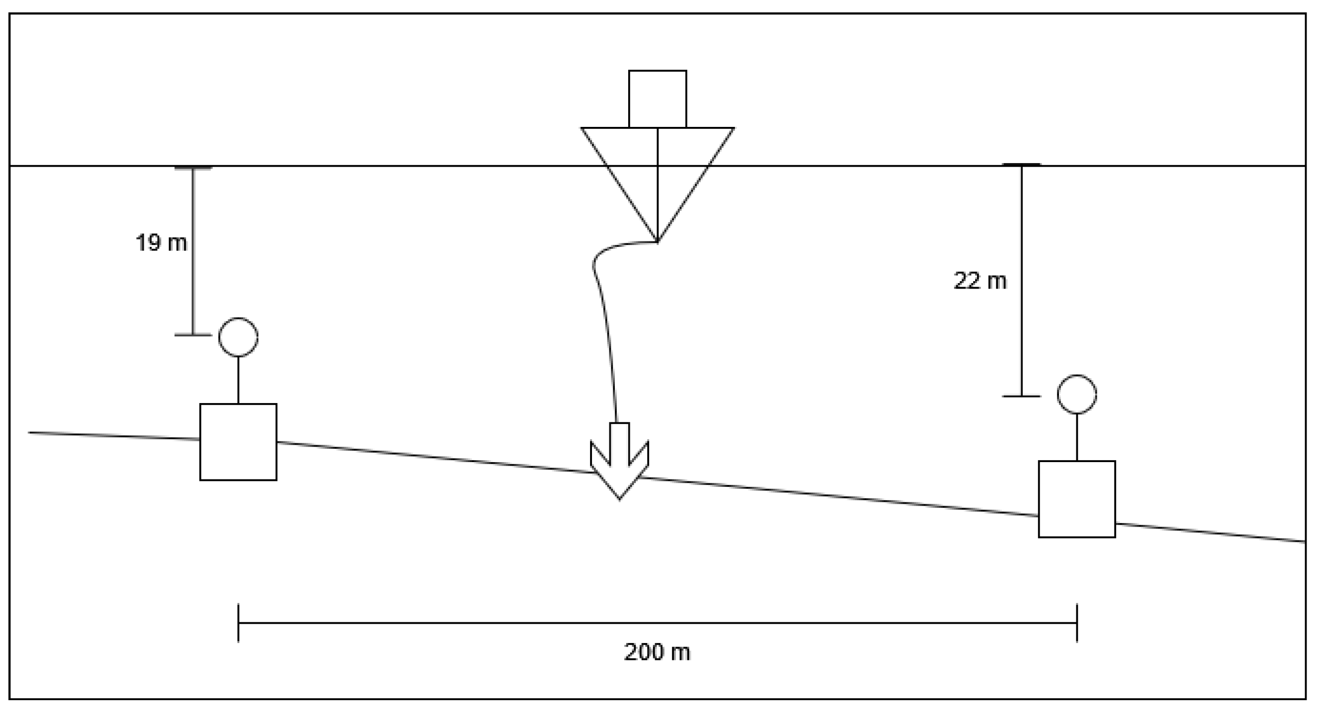
During the static range trials, PCT Moose was anchored between two hydrophones situated 200 m apart and 1 m off the sea floor. Due to the slope of the bottom, the north hydrophone is 19 m deep and the south hydrophone is 22 m deep. Figure 1 shows a diagram of the hydrophone arrangement on the seafloor of the static range. The hydrophones are Brüel & Kjær (B&K) (Copenhagen, Denmark), type 8106 hydrophones with −173 dB re 1 V/Pa sensitivity. Once securely anchored, the vessel was powered down and individual systems were powered on and run. The radiated noise for each system was recorded on both hydrophones. Due to environmental concerns, some systems could not be run, but over the course of the static range, 24 unique systems were recorded. These systems include fitted systems and a piezoelectric shaker, which was temporarily fitted to the hull framing of the ship. This shaker could be set to produce a desired frequency which would be generated directly against the hull and transmitted into the water. The list of the equipment that was recorded can be seen in Table 1. Because the ship was anchored for all static range trials at a fixed distance from the hydrophones, environmental effects such as bottom and surface reflection, the speed of sound in water, etc., were considered to be constant and did not need to be corrected for.
2.2. Dynamic Range Trials
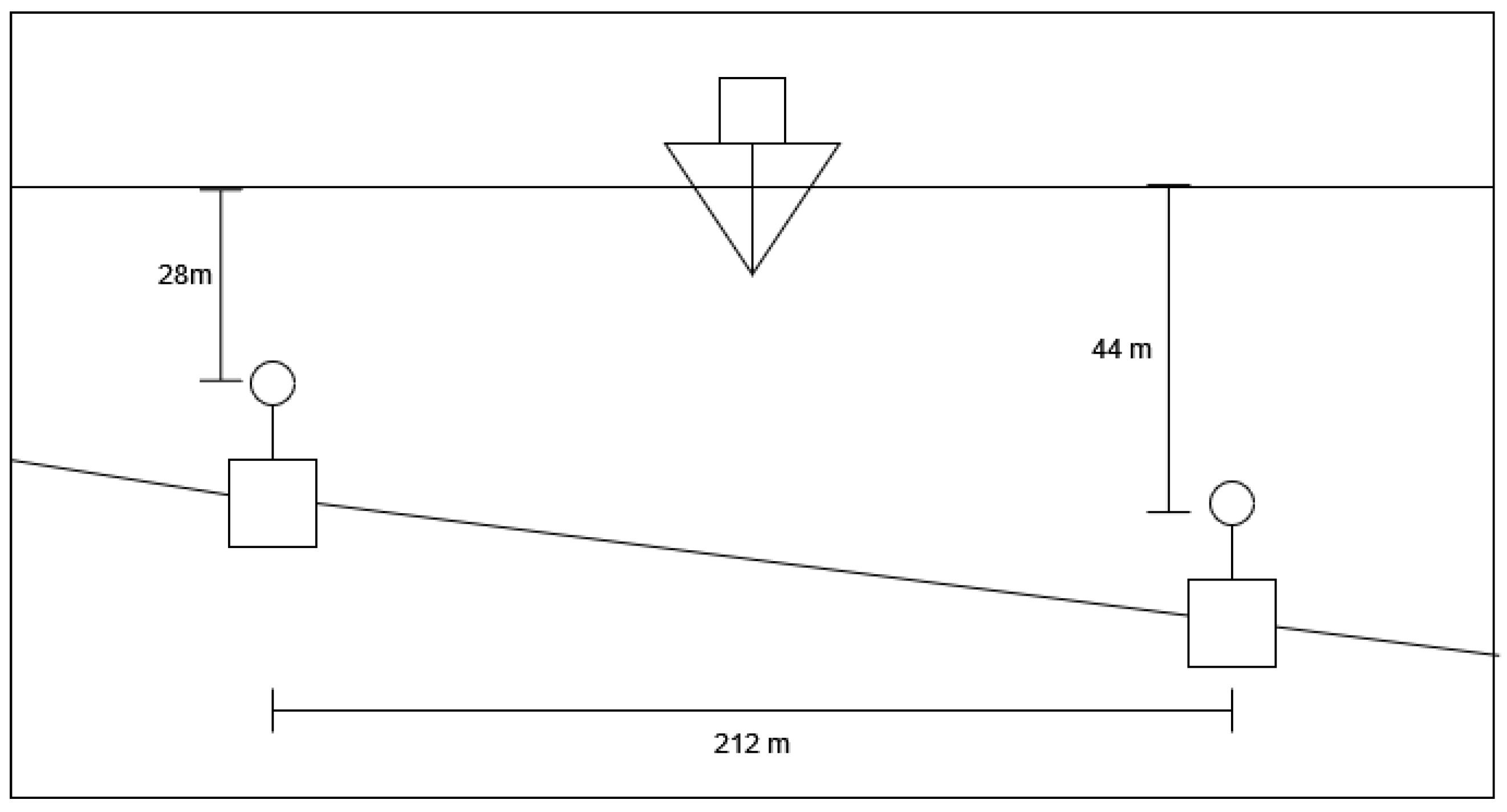
In addition to the static range trials, DRDC also conducted dynamic range trials in order to capture the total sound generated by an operational ship while propelling. The dynamic range is similarly designed to the static range, with two B&K hydrophones situated 212 m apart on the same pedestals situated 1 m from the seabed. On the dynamic range, this results in the north hydrophone resting 28 m from the surface and the south hydrophone resting 44 m from the surface. Figure 2 shows the hydrophone layout on the dynamic range. During these trials, PCT Moose was driven between the hydrophones, using the ships fitted GPS to attempt to maintain a route exactly halfway between the two hydrophones and recording any offset from this path. Each run consisted of two passes between the hydrophones, one where the ship was travelling eastward and one where it travelled westward. This allowed both hydrophones to record noise from each side of the ship. Runs were conducted at a constant speed and machinery state. Speeds were varied between runs from 3 to 20 knots and machinery states were varied based on eight possible ship system configurations. These states are detailed in Table 2. As shown in Section 4, the classifier was unable to accurately identify machinery when multiple systems were run concurrently. As a result, all trials using the dynamic range data were considered beyond the capability of the developed classifiers.
2.3. Recorded Data
The recorded sound data from all hydrophones were encoded using 32 bit integer values and recorded at a frequency of 204,800 Hz. The data were then saved in a custom binary file format where they could be losslessly converted from the flattened 32 bit integers to the hydrophone voltages. The data were also saved as a .wav format file. Since .wav files use 16 bit encoding for each sample, however, a significant amount of data were truncated at the maximum sample value. The regions of the time series where the values were truncated therefore resembled square waves which would cause spectral analysis to produce a theoretically infinite number of harmonics. As a result, the .wav file was deemed inappropriate for use in these experiments and the binary files were used.
3. Methodology
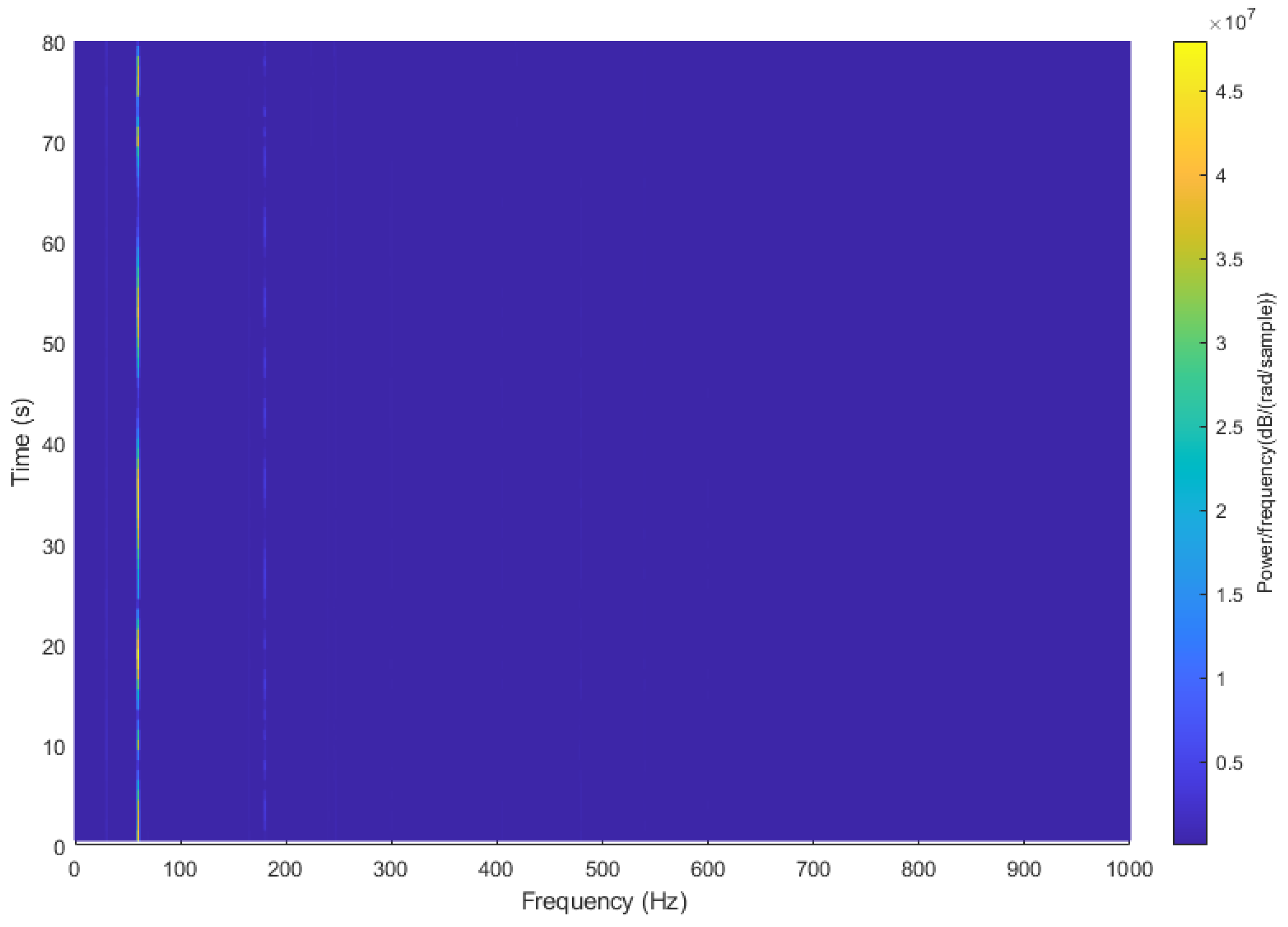
In order to examine the data and to confirm that the acoustic noise from PCT Moose demonstrates similar characteristics to those expected, spectral analysis was performed on samples of the acoustic recordings from the static range trials. A static range trial where the main fire pump was run was selected and a spectrogram was created using the Fourier transform, creating a plot with the x-axis representing time, the y-axis representing frequency, and a colour gradient representing magnitude. The results, visible in Figure 3, show that the noise of the running machine demonstrates strong line spectrum responses at 60 and 180 Hz that are clearly visible above the background noise, and are stable at constant frequencies over the entire recording. This is the anticipated spectral response for nonpropulsion-related equipment, which confirms the expectations from Section 1. With confirmation that the real hydroacoustic recordings demonstrated the necessary characteristics, sample recordings of each piece of machinery could be spectrally analyzed and examined for characteristic features.
Preliminary spectral analysis of the acoustic recordings had shown that nearly all frequencies of interest (i.e., those that were clearly discernible from the background noise) were below 2 kHz, with the exception of the piezoelectric shaker when it was set to 4 kHz. As a result, the recordings could be downsampled from 204,800 Hz to 10,240 Hz without impacting the results of the experiment.
Initially, 30 s samples of static range recordings for each system were broken into 0.1 s segments and analyzed with 1 Hz spacing for the FOS candidate frequencies. In order to limit the effect of background noise on the spectral analysis, the FOS algorithm was limited to fitting 30 terms. The fitted frequencies for each system were compared to each other in order to identify unique frequencies that were generated by only one system, which would become the identifying feature for that system. It was found, however, that 1 Hz resolution was insufficient to differentiate the systems and higher resolution would be required.
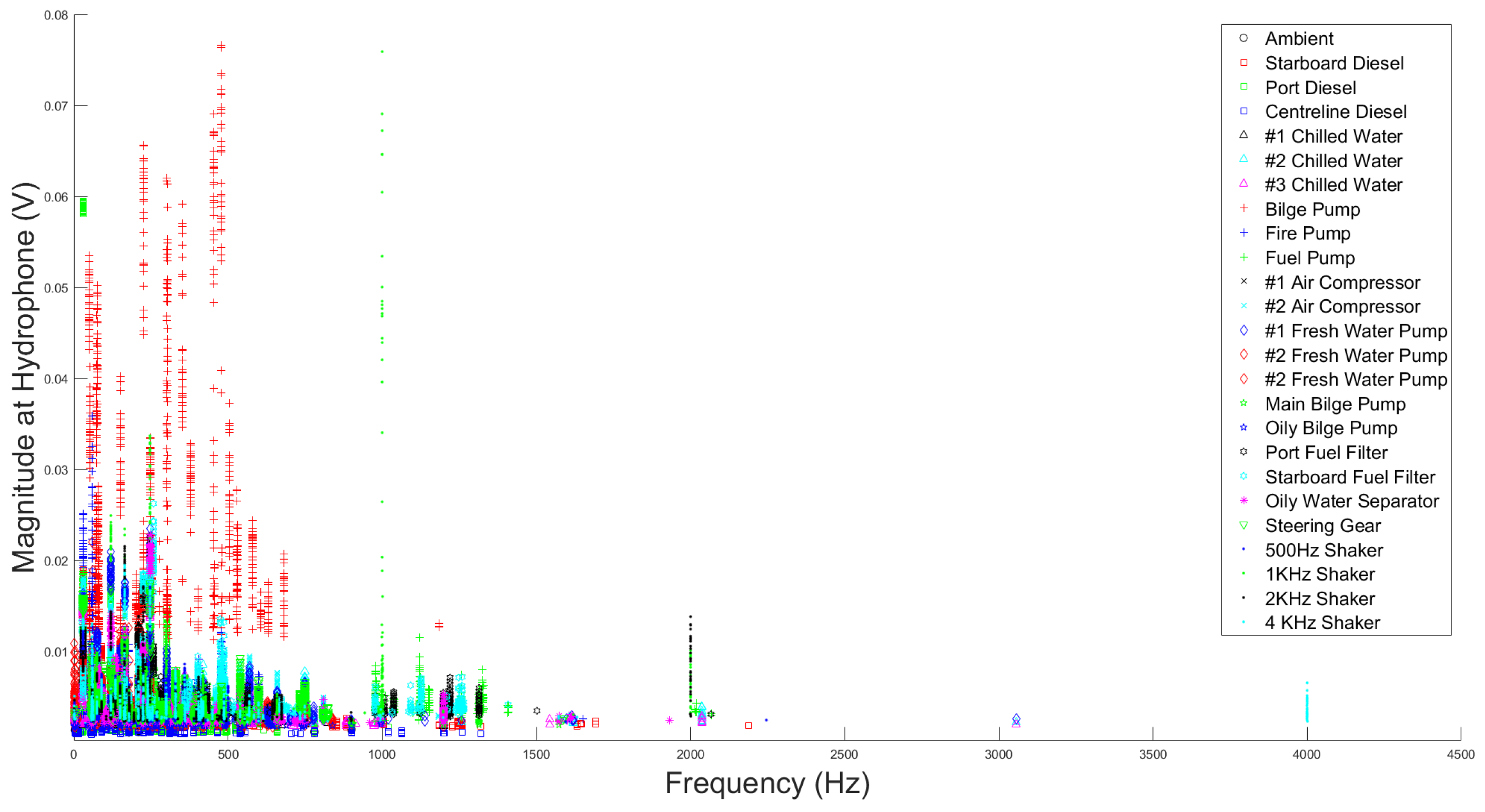
The static range recordings of each system provided by DRDC were all 93 s or 94.5 s in length; therefore, we decided to use the first 90 s of recorded data as “training data”, reserving the last 3 s of each recording for later testing. These 90 s samples were broken into 1 s segments and spectrally analyzed using FOS, with candidate functions 0.1 Hz apart. Again, the FOS algorithm was limited to fitting 30 terms. The results from each spectral analysis were then plotted on a single cluster graph with frequency and magnitude axes. Each system was given a unique colour and symbol combination, and each point in the cluster therefore represented a frequency that the system had emitted over the course of the 90 s recording. Feature frequencies for the systems could then be identified as any frequency where only one symbol was plotted. The resulting scatter plot can be seen in Figure 4, where several obvious features are apparent at a glance, such as the piezoelectric shaker clusters at 2 kHz and 4 kHz.
The cluster plot was examined in close detail for frequencies where only one system emitted energy. These frequencies were selected as representative, or feature, frequencies for their systems. It was found during this search that 0.1 Hz spectral resolution was still insufficient to separate all the systems from each other. Only 11 of the 24 possible systems were identifiable in this way. A classifier was built for these 11 systems. This single frequency classifier is based on a simple binary decision. If the unique frequency identified for any of the 11 identified systems is detected when a sample is spectrally analyzed, the system is identified as “running”; if it is not detected, the system is identified as “not running”.
In an attempt to develop features for the remaining systems, a higher-order feature set was developed. The same cluster plot from Figure 4 was re-examined for instances where a system radiated energy at two frequencies. While these two frequencies did not need to be independently occupied by the subject system, the clusters for the subject system were required to be within a unique magnitude range. That is, any other system that had energy fitted at the same frequency as the subject system did not have any instances where the fitted magnitude was within the range of fitted magnitudes for the subject system. It was also required that both these frequencies had been fitted to the functional expansion by the FOS algorithm in at least 80% of the 1 s segments that were analyzed. This ensured that enough examples of the frequency pairs existed to examine them for a statistical relationship. Three systems were found that met these criteria: the port diesel generator, the starboard diesel generator, and the #1 chilled water plant.
The magnitudes for the fitted frequency pairs in each 1 s segment were normalized against each other by dividing the individual fitted magnitudes by the sum of the two magnitudes, resulting in a ratio of magnitudes for each sample that sum to 1. The mean and standard deviation of these ratios over all 90 segments were calculated, and a frequency pair classifier was created to identify running systems. If the two feature frequencies for a system are detected by spectral analysis, the classifier normalizes their fitted magnitudes and calculates the z-score of both normalized values against the mean and standard deviation calculated from the training data using the formula:
where x is the value of an individual sample, is the sample mean, and S is the sample standard deviation. z-score is simply a count of the number of standard deviations that an individual sample is from the sample mean; therefore, if the z-scores for both the feature frequencies for the sample are less than 2, then the data conform to the training data within a 95% confidence interval and the classifier identifies the system as “running”.
The single frequency and frequency pair classifiers were then tested for their ability to accurately predict the running machinery from static and dynamic range recordings of PCT Moose. The last 3 s of static range recording from each system as well as 3 s of ambient data recorded during the static range trials were combined into a single 75 s time series and spectrally analyzed using the FOS algorithm. The classifiers were run on the resulting functional expansions to identify the running systems.
A classifier based on the FFT was then designed as a tool to compare against the single frequency classifier. This classifier conducted spectral analysis on the sample acoustic data to generate a spectral plot. The plot was then searched for local maxima and those maxima were compared to the feature frequencies for the system being tested. If any local maximum matched a system’s feature frequency, the system was deemed to be running. Since the test data was broken into 1 s segments, the maximum spectral resolution of the FFT was 1 Hz. There were seven systems for which unique frequencies were identified at 1 Hz resolution using the FOS algorithm; therefore, this comparison was limited to those seven systems.
4. Results
4.1. Single Frequency Classifier
The 75 s test data were broken into 1 s segments and spectrally analyzed using the FOS algorithm. The results were then passed through the single frequency classifier and tested for the 11 systems for which a single frequency feature had been identified. Treating each system as a unique test for each 1 s segment of hydroacoustic recording results in 825 tests, for which the system being classified was running in 50 tests and not running in the remaining 775 tests. Table 3 shows the results of this trial in a confusion matrix. Since there are two possible states for the systems and two possible classifications, there are four possible test outcomes. A confusion matrix lays out the four possible outcomes in a table with the true states along the side and the estimated states across the top of the table. The sum in the top left corner denotes the number of tests conducted in each true state. As shown in Table 3, the classifier achieved a probability of detection of , with a probability of false detection of and total probability of error of .
4.2. Comparison with FFT Classifier
In order to accurately compare the FFT classifier with the single frequency FOS classifier, it was necessary, as previously stated, to reduce the tested systems to the seven systems that were identifiable with 1 Hz frequency resolution. This reduces the number of unique tests to 525, with the target system running in 30 tests and not running in 495. Adjusting the confusion matrix for the FOS classifier for only these seven systems results in Table 4, where the probability of detection is , the probability of false detection is , and the total probability of error is .
The classifier based on the FFT at first appeared to be more effective than that of the FOS-based classifier, demonstrating a probability of detection of . It also had a probability of false detection of , leading to a total probability of error of . Table 5 shows the confusion matrix results for the FFT-based classifier, showing the much higher rate of estimating the system to be running, both when the system was running and when it was not.
4.3. Frequency Pair Classifier
The test for the frequency pair classifier was unique from the other tests run in that a feature was developed for the starboard diesel generator. This generator provided PCT Moose’s electrical power for all the other systems during the static range trial. As a result, its acoustic energy is present in all static range recordings (with the exception of the static range trials for the port and centreline diesel generators). This means that of the 225 individual tests performed by the classifiers (75 s of data tested by three different classifiers), 78 tests were performed with the subject system running and 147 with the system not running. This classifier was able to identify all three systems from the samples of that system’s static range trial data, but was unable to reliably identify the starboard diesel generator anywhere when another system was also running. This resulted in a probability of detection of , a probability of false detection of , and a false negative rate of . Table 6 shows the results for this test in a confusion matrix.
5. Discussion
The single frequency classifier based on the FOS algorithm was effective at estimating the running status of the systems for which features had been identified at 1 Hz and 0.1 Hz resolutions, achieving high probabilities of detection without suffering a commensurate high probability of false detection. This starkly contrasts the classifier based on the FFT, where a high probability of detection carried a similarly high probability of false detection and only 1 Hz resolution could be achieved, limiting the number of systems that could be detected. This highlights two of the main strengths of the FOS algorithm in the processing of hydroacoustic noise: its superior spectral resolution and its inherent ability to process noisy data.
The superior frequency resolution of the FOS algorithm allowed for more systems to be tested than the FFT-based classifier. While the frequency resolution of both systems can be improved through the use of larger sample segments, it was discussed in Section 1 that ship-radiated noises contain both dynamic sources, where the frequencies radiated will vary over time and static sources where the frequencies remain relatively invariant with time. If the sample time can be kept sufficiently short, the effects of varying frequency can be limited and the radiated noise will more closely approximate static sources and spectral analysis will be more accurate.
Because the test data were composed of real-world recordings, they naturally included a variety of background noises. The FOS algorithm was able to deal with this noise by simply limiting the terms fitted to the functional expansion. For all tests, the algorithm was limited to selecting 30 terms with which to approximate the test segment. This had the effect of limiting the number of frequencies of low energy that were captured by the algorithm, limiting the impact of background noise on the functioning of the FOS-based classifier. Without noise preprocessing, the FFT-based classifier analyzed all the energy in the signal, including that of background noise. This resulted, as was seen in Section 4, in much higher rates of false detection.
While the frequency pair classifier was generally less effective than the single frequency classifiers, it was remarkable in achieving a 0% false detection rate. It was able to correctly identify the running systems when they were running in isolation, but not when two systems were run concurrently. This suggests that the relationships between radiated frequencies could be exploited to generate more complex features for system identification, but that the relationships between these frequencies is affected by the presence of other running systems. In order to explore these relationships further, recordings of each system running in conjunction with many combinations of the other systems would have been required. This was not a part of the DRDC trials, so this could not be carried out.
Any discussion of the effectiveness of an algorithm to conduct EHM must necessarily include an examination of the computational cost of the algorithm. It has been noted that the increasing effectiveness of EHM techniques in identifying defects has driven an increase in computational complexity, which could reduce the overall usefulness of the algorithm if its processing time is driven below the threshold of real-time calculation [15]. The algorithm used in this research was written in MATLAB and was timed in order to gauge its ability to potentially operate in real time. It was found that the algorithm required an average of approximately 10 s to perform spectral analysis on 1 s of data (to a limit of 30 fitted terms). While this is significantly below the real-time threshold, the algorithm used for this study was not optimized. Several options exist to accelerate the processing of the FOS algorithm, such as employing more efficient programming languages or parallel processing, which could potentially greatly accelerate its computation. As a result, while the specific implementation of the FOS algorithm for this research would not be suited to EHM applications, the FOS algorithm itself can still be considered appropriate.
6. Conclusions
In these experiments, real-world hydroacoustic data from PCT Moose were examined and simple classifiers were built using the FFT and FOS algorithms in order to explore the possibility of using FOS-based spectral analysis as the basis for identification of a ship’s individual systems through its radiated noise. The FOS-based classifiers were seen to be more effective than that of the FFT-based classifier, indicating that the FOS algorithm is a suitable candidate for this application, but the inability to identify features for all the ship’s recorded systems using a simple frequency-based classification show that a more complex feature system must be explored. The frequency pair classifier showed that more complex features could be identified, but in order to fully explore the relationships between radiated frequencies for individual systems, many more data would need to be collected.
Ultimately, these experiments provide a proof of concept for the use of the FOS algorithm as a potential tool for spectral-analysis-based classification in hydroacoustic settings. Based on the success of this proof of concept and the current research applications for the FOS algorithm, this paper shows that an effective EHM tool that uses equipment noise could be developed. It also provides a strong argument for continued research into ship-radiated noise. In particular, it makes the argument in favour of conducting a more detailed range trial with more recorded data being taken of a broader configuration of machinery.
Author Contributions
Conceptualization, N.M., D.M. and H.E.; methodology, N.M.; software, D.M. and N.M.; validation, N.M., D.M. and H.E.; formal analysis, N.M.; investigation, N.M.; resources, D.M. and H.E.; data curation, N.M.; writing—original draft preparation, N.M.; writing—review and editing, H.E. and D.M.; visualization, N.M.; supervision, H.E. and D.M.; project administration, N.M.; funding acquisition, H.E. All authors have read and agreed to the published version of the manuscript.
Funding
This research received no external funding.
Data Availability Statement
Restrictions apply to the availability of these data. Data were obtained from Defence Research and Development Canada and are available from the authors with the permission of Defence Research and Development Canada.
Acknowledgments
The authors would like to thank Defence Research and Development Canada for the provision of the data used in this research, as well as their support in developing the necessary data decoding algorithms.
Conflicts of Interest
The authors declare no conflict of interest.
Abbreviations
The following abbreviations are used in this manuscript:
| B&K | Brüel & Kjær |
| DRDC | Defence Research and Development Canada |
| EHM | Equipment health monitoring |
| FFT | Fast Fourier transform |
| FOS | Fast orthogonal search |
| GS | Gram–Schmidt |
| IMF | Intrinsic mode function |
| MSE | Mean square error |
| PCT | Patrol craft, training |
| SHM | Structural health monitoring |
| SRN | Ship-radiated noise |
| WGN | White Gaussian noise |
Appendix A. The FOS Algorithm
The FOS algorithm estimates the functional expansion of a given signal using a subset of a list of arbitrary candidate functions [16]. This expansion can be written as [17]:
where is the input signal, is the weight assigned to the arbitrary function , and is a residual error.
There is no requirement for the arbitrary functions to be orthogonal; however, the fitting of orthogonal functions ensures that each function is only fit based on its unique energy. In order to accomplish this, the FOS algorithm first fits a series of orthogonal functions into a functional expansion given by the formula [17]:
where are the orthogonal functions, are the orthogonal weights, and is the residual error. The orthogonal functions are derived from the arbitrary candidate functions via Gram-Schmidt (GS) orthogonalization [16]. The formula for this process is
where are the GS orthogonalization weights and , , and are the same as in Equations (A2) and (A3). The GS orthogonalization weight for an orthogonal function, , can be obtained via [17]:
where the variables are, again, as before, and the overbar is used to indicate the time average of the underlying products. The processing time of the FOS algorithm is accelerated via the use of implicit calculation to derive the orthogonal functions. The variable is used for this implicit calculation and is defined as [17]
The correlation of is iteratively acquired by rearrangement of Equation (A3) [17]:
and simplifying to
Iterative calculation is also be used to determine via
The results from Equation (A7) can be inserted into this equation, and with simplification, the following formula is derived:
An implicitly derived can be calculated by combining Equations (A5) and (A9) and substituting into Equation (A4):
The residual error term from Equation (A1) can be used to calculate the MSE between the estimated functional expansion and the input signal. Rearranging Equation (A1) to isolate the residual error and modifying it to be the MSE yields the following formula [18]:
GS othogonalization does not change the MSE relationship of the system; therefore, MSE can also be expressed as [18]
This formula can be rearranged in order to calculate the values for each candidate function that will minimize MSE [17]:
As a result of having calculated implicitly, must also be implicitly calculated. For this, the variable is used, which is defined as [17]:
Further recursive calculation is required to produce , which is achieved via the formula
which simplifies to
Substituting to Equation (A13) then produces an implicit calculation of :
The variable Q is defined as the product of the squares of any orthogonal function and its GS orthogonalization weight. In other terms, it is the measure of the MSE reduction between the FOS estimation and the input signal that would result from adding the term to the functional expansion. The formula for calculating Q is
The candidate function with the largest Q value would provide the greatest MSE reduction between the functional expansion and the input signal. It is therefore fitted to the functional expansion first. Since it is only possible to fit a candidate function once, it is removed from the list of candidate functions, and the remaining MSE between the input signal and the functional expansion is reduced by Q.
This process is repeated; the candidate function with the highest Q value without reducing the MSE below zero (indicating that there is more energy in the functional expansion than in the input signal) is fitted to the functional expansion. This continues until a predetermined stopping criterion is met, at which time the orthogonal functions and weights can be converted back to candidate functions and their respective weights. Candidate function weights, , are derived from the orthogonal function weights, . The formula for this is [19]
where is a weighted sum of the previously calculated GS orthogonal weights. This can be calculated by [19]
To perform spectral analysis via the FOS algorithm, candidate frequencies, , are selected and matched sine and cosine pairs are generated via [17]
which then form the candidate function list. The FOS algorithm uses the combined Q of each cosine/sine pair when determining the candidate functions with the greatest MSE reduction, which are then fitted as the and terms.
Sine and cosine pairs can be converted into a into a single function with magnitude, , and phase, , given by [17]:
References
- Fahy, F.; Walker, J. Fundamentals of Noise and Vibration; Taylor & Francis: London, UK, 1998. [Google Scholar]
- Urick, R.J. Principles of Underwater Sound; McGraw-Hill: New York, NY, USA, 1975. [Google Scholar]
- Li, Y.; Ning, F.; Jiang, X.; Yi, Y. Feature Extraction of Ship Radiation Signals Based on Wavelet Packet Decomposition and Energy Entropy. Math. Probl. Eng. 2022, 2022, 8092706. [Google Scholar] [CrossRef]
- Li, R.; Bu, W.; Cheng, J. Research on Ship-radiated Noise Evaluation and Experiment Based on OTPA Optimized by Operation Clustering. In Proceedings of the 2021 OES China Ocean Acoustics (COA), Harbin, China, 14–17 July 2021; pp. 450–455. [Google Scholar]
- Yang, H.; Li, L.; Li, G.; Guan, Q. A Novel Feature Extraction Method for Ship-radiated Noise. Def. Technol. 2022, 18, 604–617. [Google Scholar] [CrossRef]
- Farrokhrooz, M.; Karimi, M. Marine Vessels Acoustic Radiated Noise Classification in Passive Sonar Using Probabilistic Neural Network and Spectral Features. Intell. Autom. Soft Comput. 2011, 17, 369–383. [Google Scholar] [CrossRef]
- Li, G.; Hou, Y.; Yang, H. A Novel Method for Frequency Feature Extraction of Ship Radiated Noise Based on Variational Mode Decomposition, Double Coupled Duffing Chaotic Oscillator and Multivariate Multiscale Dispersion Entropy. Alex. Eng. J. 2022, 61, 6329–6347. [Google Scholar] [CrossRef]
- Li, Y.; Li, Y.; Chen, X.; Yu, J. A Novel Feature Extraction Method for Ship-Radiated Noise Based on Variational Mode Decomposition and Multi-Scale Permutation Entropy. Entropy 2017, 19, 342. [Google Scholar] [CrossRef]
- Peng, C.; Yang, L.; Jiang, X.; Song, Y. Design of a Ship Radiated Noise Model and its Application to Feature Extraction Based on Winger’s Higher-Order Spectrum. In Proceedings of the 2019 IEEE 4th Advanced Information Technology, Electronic and Automation Control Conference (IAEAC), Chengdu, China, 20–22 December 2019; Volume 1, pp. 582–587. [Google Scholar]
- McGaughey, D.R.; Dagenais, V.; Pecknold, S.P. Improved Torpedo Range Estimation Using the Fast Orthogonal Search. IEEE J. Ocean. Eng. 2010, 35, 595–602. [Google Scholar] [CrossRef]
- Chon, K. Accurate identification of periodic oscillations buried in white or colored noise using fast orthogonal search. In Proceedings of the First Joint BMES/EMBS Conference, 1999 IEEE Engineering in Medicine and Biology 21st Annual Conference and the 1999 Annual Fall Meeting of the Biomedical Engineering Society (Cat. N), Atlanta, GA, USA, 13–16 October 1999; Volume 2, p. 998. [Google Scholar]
- El-Shafie, A.; Noureldin, A.; McGaughey, D.; Hussain, A. Fast orthogonal search (FOS) versus fast Fourier transform (FFT) as spectral model estimations techniques applied for structural health monitoring (SHM). Struct. Multidiscip. Optim. 2012, 45, 503–513. [Google Scholar] [CrossRef]
- King, G.; Tarbouchi, M.; McGaughey, D. Rotor Fault Detection in Induction Motors Using the Fast Orthogonal Search Algorithm. In Proceedings of the 2010 IEEE International Symposium on Industrial Electronics, Bari, Italy, 4–7 July 2010; pp. 2621–2625. [Google Scholar]
- Thongam, J.S.; Tarbouchi, M.; Okou, A.F.; Bouchard, D.; Beguenane, R. Electric Ship Propulsion Drive Motors—A Review of the Present State of the Art. In Proceedings of the 2013 Eighth International Conference and Exhibition on Ecological Vehicles and Renewable Energies (EVER), Monte Carlo, Monaco, 27–30 July 2010; pp. 1–8. [Google Scholar]
- Bellini, A.; Filippetti, F.; Tassoni, C.; Capolino, G.A. Advances in Diagnostic Techniques for Induction Machines. IEEE Trans. Ind. Electron. 2008, 55, 4109–4126. [Google Scholar] [CrossRef]
- Korenberg, M.J. Fast Orthogonal Algorithms for Nonlinear System Identification and Time-Series Analysis. In Advanced Methods of Physiological System Modeling; Springer: New York, NY, USA, 1989; pp. 165–177. [Google Scholar]
- McGaughey, D.R.; Tarbouchi, M.; Nutt, K.; Chikhani, A. Speed Sensorless Estimation of AC Induction Motors Using the Fast Orthogonal Search Algorithm. IEEE Trans. Energy Convers. 2006, 21, 112–120. [Google Scholar] [CrossRef]
- Korenberg, M.J.; Paarmann, L.D. Applications of Fast Orthogonal Search: Time-Series Analysis and Resolution of Signals in Noise. Ann. Biomed. Eng. 1989, 17, 219–231. [Google Scholar] [CrossRef] [PubMed]
- Korenberg, M.J. A Robust Orthogonal Algorithm for System Identification and Time-Series Analysis. Biol. Cybern. 1989, 60, 267–276. [Google Scholar] [CrossRef] [PubMed]
Figure 1.
Static range hydrophone configuration.

Figure 2.
Dynamic range hydrophone configuration.

Figure 3.
Static range spectrogram (in dB) of fire pump operation.

Figure 4.
Cluster plot of spectral analysis using FOS.


Table 1.
Unique systems recorded during static range trials.
| Port Diesel generator | #2 Air Compressor |
| Centreline diesel generator | Oily water separator |
| Starboard diesel generator | Main bilge pump |
| Main fire pump | Oily bilge pump |
| Emergency fire pump | Steering gear hydraulic system |
| Fuel oil transfer pump | #1 Fresh water pump with hot water pump |
| Port fuel filter coalescer | #2 Fresh water pump with hot water pump |
| Starboard fuel filter coalescer | Engine room cooling fan |
| #1 Chilled water condenser | Piezoelectric shaker (500 Hz) |
| #2 Chilled water condenser | Piezoelectric shaker (1 kHz) |
| #3 Chilled water condenser | Piezoelectric shaker (2 kHz) |
| #1 Air compressor | Piezoelectric shaker (4 kHz) |
Table 2.
Machinery states during dynamic range trials.
| Machinery State | |||
|---|---|---|---|
| A | Normal | E | Two generators (centreline and starboard) |
| B | Main fire pump on | F | Bilge pump (cycling on/off) |
| C | Secondary generator (centreline) | G | Trailing port propeller |
| D | Tertiary generator (port) | H | Trailing starboard propeller |
Table 3.
Confusion matrix results from single frequency classifier test.
| Estimated Status | |||
|---|---|---|---|
| Total 50 + 775 = 825 | Running | Not Running | |
| Actual Status | Running | 33 | 17 |
| Not Running | 6 | 769 | |
Table 4.
Adjusted confusion matrix results from single frequency classifier test.
| Estimated Status | |||
|---|---|---|---|
| Total 30 + 495 = 525 | Running | Not Running | |
| Actual Status | Running | 21 | 9 |
| Not Running | 2 | 493 | |
Table 5.
Confusion matrix results from FFT trial.
| Estimated Status | |||
|---|---|---|---|
| Total 30 + 495 = 525 | Running | Not Running | |
| Actual Status | Running | 29 | 1 |
| Not Running | 304 | 191 | |
Table 6.
Confusion matrix results from frequency pair classifier.
| Estimated Status | |||
|---|---|---|---|
| Total 78 + 147 = 225 | Running | Not Running | |
| Actual Status | Running | 12 | 66 |
| Not Running | 0 | 147 | |
Disclaimer/Publisher’s Note: The statements, opinions and data contained in all publications are solely those of the individual author(s) and contributor(s) and not of MDPI and/or the editor(s). MDPI and/or the editor(s) disclaim responsibility for any injury to people or property resulting from any ideas, methods, instructions or products referred to in the content. |
© 2023 by the authors. Licensee MDPI, Basel, Switzerland. This article is an open access article distributed under the terms and conditions of the Creative Commons Attribution (CC BY) license (https://creativecommons.org/licenses/by/4.0/).
Share and Cite
MDPI and ACS Style
Marasco, N.; Elghamrawy, H.; McGaughey, D. Using Feature Extraction to Perform Equipment Health Monitoring on Ship-Radiated Noise. Acoustics 2023, 5, 1180-1193. https://doi.org/10.3390/acoustics5040067
AMA Style
Marasco N, Elghamrawy H, McGaughey D. Using Feature Extraction to Perform Equipment Health Monitoring on Ship-Radiated Noise. Acoustics. 2023; 5(4):1180-1193. https://doi.org/10.3390/acoustics5040067
Chicago/Turabian StyleMarasco, Nicholas, Haidy Elghamrawy, and Donald McGaughey. 2023. "Using Feature Extraction to Perform Equipment Health Monitoring on Ship-Radiated Noise" Acoustics 5, no. 4: 1180-1193. https://doi.org/10.3390/acoustics5040067