FEM Modeling of Electro-Acoustic Nonlinearities in Surface Acoustic Wave Devices: A Methodological Review

Abstract

In the framework of electro-elasticity theory and the finite element method (FEM), a model is set up for the computation of quantities in surface acoustic wave (SAW) devices accounting for nonlinear effects. These include second-order and third-order intermodulations, second and third harmonic generation and the influence of electro-acoustic nonlinearity on the frequency characteristics of SAW resonators. The model is based on perturbation theory, and requires input material constants, e.g., the elastic moduli up to fourth order for all materials involved. The model is two-dimensional, corresponding to an infinite aperture, but all three Cartesian components of the displacement and electrical fields are accounted for. The first version of the model pertains to an infinite periodic arrangement of electrodes. It is subsequently generalized to systems with a finite number of electrodes. For the latter version, a recursive algorithm is presented which is related to the cascading scheme of Plessky and Koskela and strongly reduces computation time and memory requirements. The model is applied to TC-SAW systems with copper electrodes buried in an oxide film on a LiNbO₃ substrate. Results of computations are presented for the electrical current due to third-order intermodulations and the displacement field associated with the second harmonic and second-order intermodulations, generated by monochromatic input tones. The scope of this review is limited to methodological aspects with the goal to enable calculations of nonlinear quantities in SAW devices on inexpensive and easily accessible computing platforms.

1. Introduction

Signal processing devices based on surface acoustic waves (SAW), like frequency filters, delay lines and others, have, nowadays, far-reaching applications in various fields, especially in the growing market of mobile communication. The working principle of almost all these devices makes use of the piezoelectric effect with interdigital electrode structures and relies on linear behavior. New standards like 5G further raise the linearity requirements. This has led to an urgent need for gaining an in-depth understanding of the influence of nonlinearity on the propagation of SAWs and for means to reduce this influence.

Major undesired nonlinear effects that occur in SAW devices and need to be counteracted are harmonic generation and intermodulations, which can deteriorate signal quality in mobile communication. Of similar importance is the power dependence of the resonance frequencies. All these effects will be addressed in this review.

So far, modelling of nonlinear effects in SAW devices has mostly been carried out phenomenologically by extending coupling of modes (COM) and P-matrix theory [1,2,3,4] or by nonlinear extensions of an equivalent circuit model (especially the Mason model) [5]. The latter were successfully applied to bulk acoustic wave (BAW) devices [6,7] (and references therein). Parameters containing information on nonlinearity were obtained by fitting to experimental data. Calculations, relating nonlinear effects like third-order intermodulational distortions (IMD3) directly to linear and nonlinear material constants of the elastic media involved, use the finite element method (FEM) [8,9,10,11,12,13,14,15]. In contrast to the phenomenological models mentioned above, finite element calculations do not rely on restrictive model assumptions. They yield reliable results without the need for fit parameters, if the relevant material constants are known to a sufficient extent and accuracy. In addition, they provide full-wave fields, which can be very useful for the designer of SAW devices and allow for detailed insights into the nonlinear behavior of a device.

To the authors’ knowledge, detailed investigations of nonlinear propagation effects in connection with SAWs began in the mid-sixties of the previous century (for a review see [16]). The field was boosted by the development of the elastic convolver, an analog, nonlinear, signal-processing device based on SAWs, which, however, did not reach the market (see the reviews [17,18]). Here, electro-acoustic nonlinearity was a desired effect. Nonlinearity in the context of SAWs has gained renewed attention in connection with further miniaturization, leading to higher power densities, and tightened linearity requirements for signal processing devices, as well as in the field of non-destructive evaluation [19].

The major “classical” sources of nonlinearity are the third- and higher-order terms in an expansion of the materials’ potential energy per unit volume in powers of displacement gradients and electrical field components. The theory of nonlinear electro-elasticity was presented in detail in classical texts [20,21,22,23]. Theoretical studies of effects of this classical nonlinearity on the propagation of surface acoustic waves were first carried out with the help of coupled amplitude equations, derived by Reutov [24], or evolution equations in the form of integral equations ([25] and references therein). They focused on homogeneous media and layered structures, including piezoelectric materials, with planar surfaces and interfaces. They allowed for simulations and, hence, for quantitative predictions of nonlinear propagation effects directly on the basis of material constants. The investigations included intermodulations at an early stage [26,27].

The complexity of the displacement field and the spatial distribution of electrostatic potential in SAW-based devices with their arrangements of electrodes on the surface or buried in a dielectric film calls for the use of numerical techniques, such as FEM for quantitative predictions of nonlinear effects. The goal of this review paper is to outline, in detail, a two-dimensional FEM-based approach, treating the nonlinearity within perturbation theory. To demonstrate its applicability to quantitative analysis of electrical currents and mechanical displacements generated by the electro-elastic nonlinearities of the constituent materials of a SAW device, a few numerical results are shown, which refer to a temperature-compensated SAW system (TC-SAW system) consisting of copper electrodes on a LiNbO₃ 128°YX substrate and a silicon oxide film. The presentation focuses on methods and algorithms rather than on numerical results. The complexity of the simulation methods and their theoretical basis in nonlinear electro-elasticity induced us to confine this review to methodological aspects concerning theory rather than including experimental results or giving a detailed overview of the field’s historical development.

The paper is structured in the following way:

In Section 2, the part of nonlinear elasticity theory underlying the FEM model is briefly summarized, and the notation used in the following sections is introduced. In particular, we introduce a four-component generalized displacement field, its fourth component being the electrostatic potential. In this context, the material constants used as input data in the numerical calculations for the considered TC-SAW system are mentioned and their sources provided.

Section 3 presents the FEM model itself for an infinite periodic arrangement of electrodes and for a finite number of electrodes.

In Section 4, two different methods of calculating the current in the electrodes due to third-order intermodulations are introduced. One of them allows the calculation of the nonlinear current generated by third-order intermodulations without first determining the displacement field and electrostatic potential associated with the third-order intermodulations.

In Section 5, we show how the influence of nonlinearity on the resonance curve and phase response of a SAW resonator can be efficiently determined by combining FEM with perturbation theory.

In Section 6, reflections of bulk waves from the bottom of the substrate are considered, which are part of the (generalized) displacement field of the second harmonic of a SAW excited in an interdigital transducer.

Section 7 is concerned with FEM calculations for systems with a finite number of equidistantly arranged electrodes. A recursive algorithm is introduced that enables calculations of nonlinear quantities (mechanical and electrical displacement fields associated with intermodulations and higher harmonics) for a large number of electrodes with considerably reduced numerical effort as compared to the standard approach. The paper ends with a short conclusion.

2. Nonlinear Electro-Elasticity

2.1. General Theory

The theory of nonlinear electro-elasticity underlying our FEM calculations was developed in detail in the nineteen-sixties to eighties (see, e.g., [20,21,22,23,25]). Here, only a brief summary is provided. Further references to earlier work may be found in [16,23].

As degrees of freedom, we consider the three Cartesian components of the displacement field, u₁, u₂, u₃, referring to the spatial frame [20] and the electrical potential. The latter will be treated as the fourth component, u₄, of a four-component generalized displacement field. This concept was introduced for linear piezoelectricity in [28] and was applied to nonlinearity in [25,29,30,31,32]. The components of the generalized displacement field are labelled by lower-case Latin indices. They depend on time t and on the Cartesian coordinates X₁, X₂, X₃, referring to the material frame [20] and being the Cartesian components of the position vector X. We invoke a summation convention that implies summation over repeated lower-case Latin indices from 1 to 4 and summation over repeated upper-case Latin indices from 1 to 3. These indices are always subscripts. (We note that there is no implicit summation over any other kind of index.).

The equations of motion and, partly, the boundary conditions for the four-component generalized displacement field can be derived from a Lagrangian,

$$L={\displaystyle \int }\left(T-\Phi \right) d^3\mathit{X} ,$$

(1)

via Hamilton’s principle (see for example [20,23,33]). In (1), $d^3\mathit{X}$ denotes the volume element in material coordinates, and the integral extends over the entire space filled with elastic material. The kinetic energy per unit volume of undeformed elastic medium is

$$T=\frac{1}{2} \rho \left(\mathit{X}\right)\left(\frac{\partial }{\partial t}{u}_m\left(\mathit{X},t\right)\right){\mathsf{\Delta }}_{mn}\left(\frac{\partial }{\partial t}{u}_n\left(\mathit{X},t\right)\right).$$

(2)

Consequently, $\rho \left(\mathit{X}\right)$ is the mass density at position X of the undeformed medium. Furthermore, ${\Delta }_{mn}$ is a generalized Kronecker symbol defined as ${\Delta }_{mn}=1,$ if m = n and $m\ne 4$, and ${\Delta }_{mn}=0$ otherwise.

For the systems we are considering here, which consist of elastic and partially piezo-electric media, it is assumed that the potential energy per unit volume of the undeformed medium,$\Phi$, may be expanded in powers of gradients of the generalized displacement field components $u_{j,M}\left(\mathit{X},t\right)=\partial u_j\left(\mathit{X},t\right)/\partial {\mathit{X}}_M$,

$$\begin{gathered} \Phi =\frac{1}{2!}{C}_{mM nN}{u}_{m,M}{u}_{n,N}+\frac{1}{3!}{S}_{mM nN pP}^{\left(2\right)}{u}_{m,M}{u}_{n,N}{u}_{p,P} \\ +\frac{1}{4!}{S}_{mM nN pP qQ}^{\left(3\right)}{u}_{m,M}{u}_{n,N}{u}_{p,P}{u}_{q,Q}+O\left(u_{\dots }^5\right). \end{gathered}$$

(3)

The expansion coefficients on the right-hand side of (3) may be regarded as components of generalized tensors C, S⁽²⁾, S⁽³⁾, which may depend on position X. In order to avoid confusion, we note that the superscripts ⁽²⁾ and ⁽³⁾ in the above equation refer to second-order (i.e., lowest-order) and third-order nonlinearity, respectively, and do not correspond to the order in the expansion of $\Phi$ in powers of generalized displacement gradient components. For simplicity, we only treat cases where the system is in static equilibrium, where no external static stress or electric field is applied to the system. In such cases, the expansion coefficients in the first term on the right-hand side of (3) have the following meaning:

For the indices m, n ranging from 1 to 3, $C_{mM nN}$ are second-order elastic constants (SOECs). $C_{4M lN}=C_{lN 4M}={\delta }_{lL} e_{M LN}, l=1,2,3; M,N,L=1,2,3,$ are the linear piezoelectric constants, and $C_{4M 4N}=-{\epsilon }_{NM}$, apart from the minus-sign, are the static dielectric constants of the corresponding medium.

In the second term on the right-hand side of (3), $S_{mM nN pP}^{\left(2\right)}$are linear combinations of second-order and third-order elastic constants (TOECs), if the indices m, n, p range between 1 and 3. The coefficients $S_{4M nN pP}^{\left(2\right)}$ with n, p ranging between 1 and 3 are linear combinations of electro-elastic and piezoelectric constants; $S_{4M 4N pP}^{\left(2\right)}$ with p = 1,2,3, are related to the electrostriction constants, and $S_{4M 4N 4P}^{\left(2\right)}$ to the static second-order electrical permittivities.

In the third term on the right-hand side of (3), $S_{mM nN pP qQ}^{\left(3\right)}$ are linear combinations of second-order, third-order and fourth-order elastic constants (FOECs), if the lower-case indices m, n, p, q range between 1 and 3 [34]. If at least one of the indices m, n, p, q is equal to 4, the corresponding coefficient is related to the electrical potential. All fourth-order material constants entering the generalized eighth-rank tensor S⁽³⁾ are specified in [23]. (For further details, see [16,20,23,25,34].) Explicit expressions for the elements of the tensors S⁽²⁾, S⁽³⁾ in terms of the material constants are provided in the Appendix A.

We note that the index pairs, consisting of a lower-case and an upper-case index, may be permuted at the quantities $C_{kM lN}, S_{mM nN pP}^{\left(2\right)},$ and $S_{mM nN pP qQ}^{\left(3\right)}$.

2.2. Input Data for the TC-SAW System

In order to obtain reliable results in FEM simulations, all material constants entering the generalized tensors C, S⁽²⁾ and S⁽³⁾ must be known for the materials that constitute the device to be modelled. For the example system of a TC-SAW interdigital transducer considered here, these are 128° rotated Y-cut LiNbO₃ as substrate material (Euler angles: λ = 0.0°, μ = 37.85°, θ = 0.0°), copper electrodes and a temperature-compensating silicon oxide film, which covers the electrodes and the substrate surface. For simplicity, the surface of the SiO₂ film is taken to be planar in our model. A complete set of material constants occurring in C, S⁽²⁾ and S⁽³⁾ is hardly available for any material. The situation for the three materials in our example system will now be discussed.

2.2.1. Material Constants for LiNbO₃

The second-order elastic constants, piezoelectric constants and dielectric constants entering the generalized tensor C were taken from [35]. For the third-order material constants (TOECs, electro-elastic constants, electrostriction constants and second-order electrical permittivities) a complete set of measured data is available [36] and was used in the generalized tensor S⁽²⁾, along with the linear material constants of [35]. Since no fourth-order material constants for LiNbO₃ are known to us, we have equated the generalized tensor S⁽³⁾ to zero in most of our calculations of IMD3. To demonstrate the role of the material constants of second and third order in the tensor S⁽³⁾, we compare, in Section 4, the results for IMD3 and the third harmonic obtained when equating S⁽³⁾ to zero, with those obtained with S⁽³⁾ containing certain second-order and third-order, but no fourth-order material constants.

As a caveat, we would like to mention here that substantial compensations of material constants of different orders can occur in the tensors S⁽²⁾ and S⁽³⁾. In order to account for the unknown FOECs in a rough approximate way, an isotropic approximation was introduced in [15], and the four fourth-order Lamé constants were treated as fit parameters. For the mass density of LiNbO₃, we chose the value of 4628 kg/m³.

2.2.2. Material Constants for SiO₂

The two second-order elastic constants and mass density of the isotropic SiO₂ film are provided in [37] (second row in Table II). Our sources for the three TOECs are [38,39] and for the four FOECs [40]. For the static relative dielectric constant, the value 3.75 was chosen. All third-order and fourth-order material constants related to the electrostatic potential either vanish or have been neglected. We note that the material constants of the SiO₂ film may be sensitive to its fabrication process. Yost and Breazeale [39] point out that residual stress has a considerable influence on the TOECs of SiO₂.

2.2.3. Material Constants for Copper Electrodes

As mentioned above, subtle compensations between elastic constants of different order may occur in the generalized tensors S⁽²⁾ and S⁽³⁾. Therefore, a consistent data set of material constants is desirable, which is obtained from the same source. In the case of crystalline copper, such a data set is available from ab-initio calculations based on density functional theory [41]. Good agreement for second-order and third-order elastic moduli was found between the ab-initio results and measured data. All FOECs are provided in [41], too. These constants have been isotropized by averaging using the Voigt assumption [42,43]. The mass density value chosen for our calculations was 8920 kg/m³.

3. FEM Modeling of Nonlinear SAW Systems

3.1. General Considerations

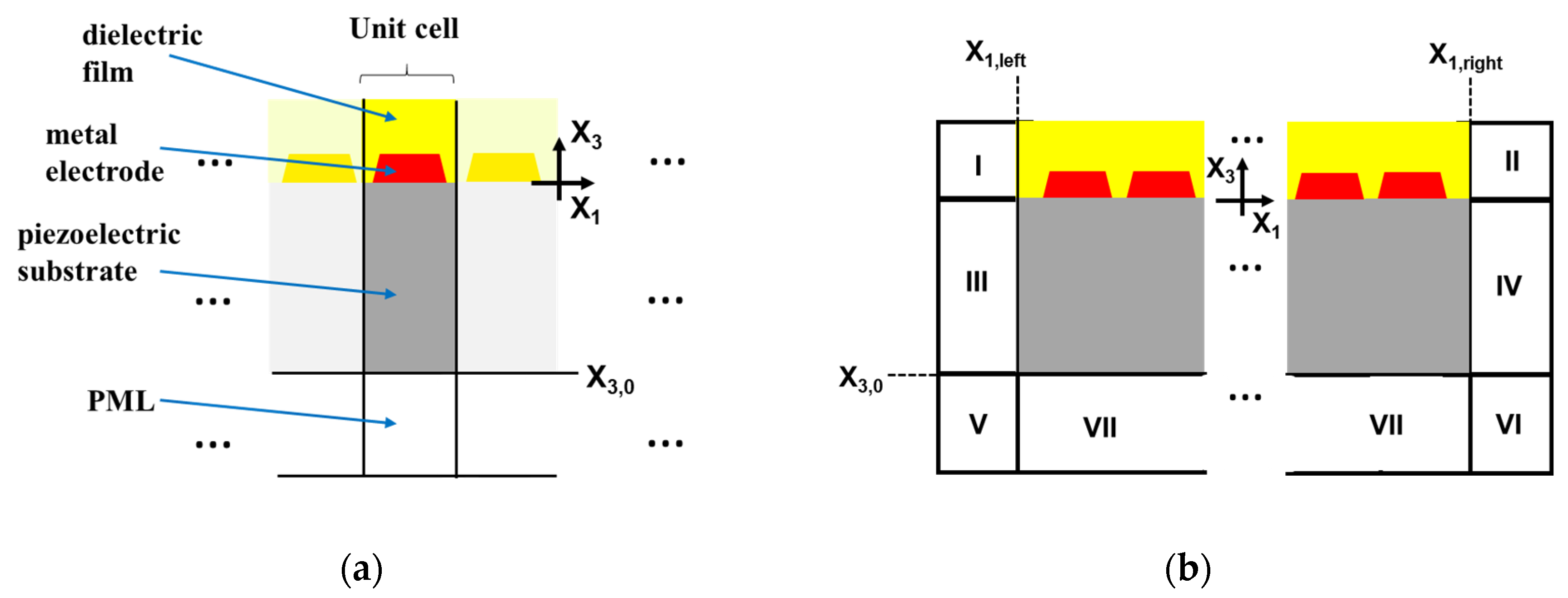
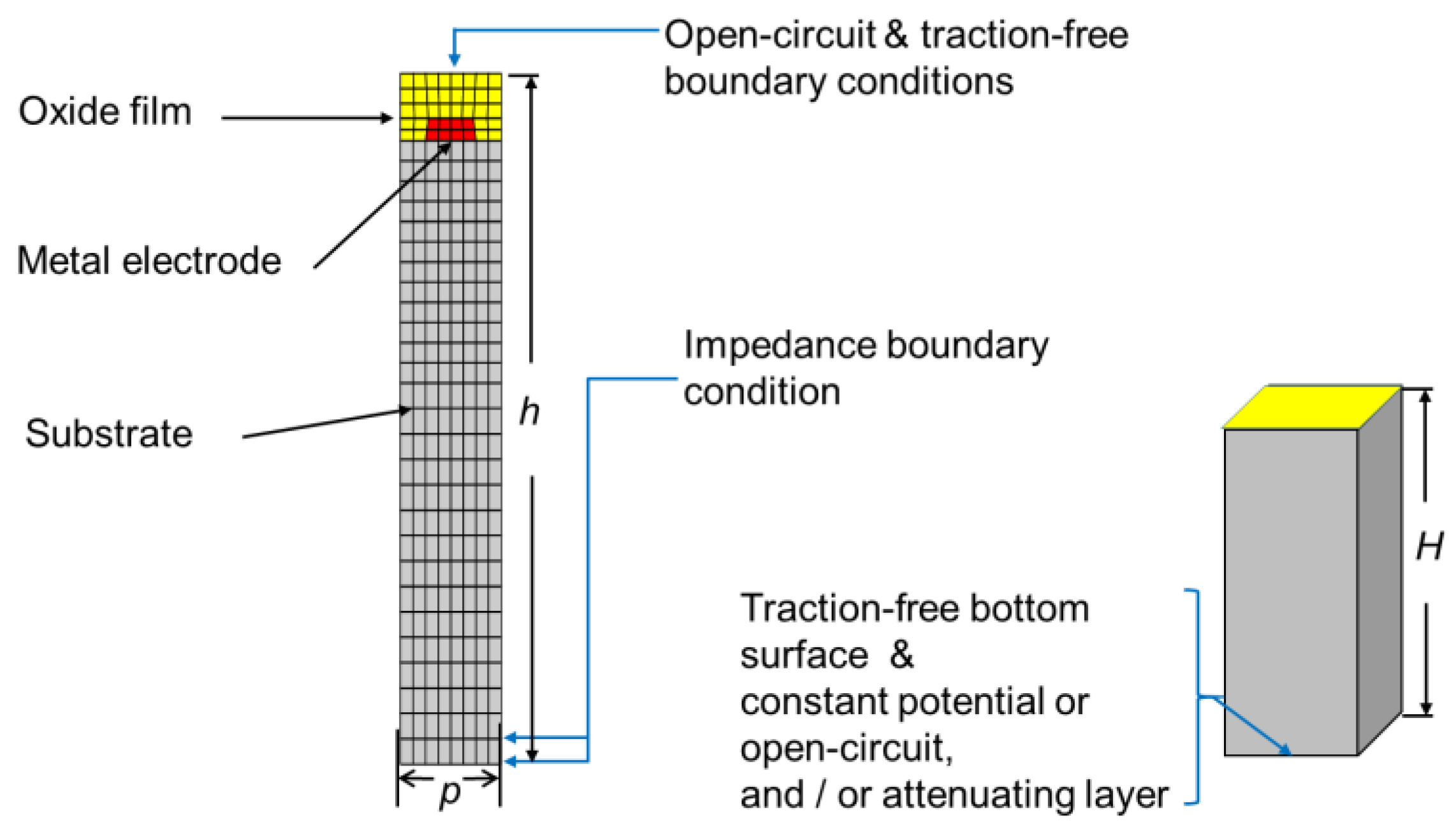
Our FEM modeling of SAW systems was confined to two dimensions, assuming an infinite aperture of the electrodes and no dependence of the displacement field and electric potential on X₂ in the coordinate system introduced in Figure 1. However, all three Cartesian components of the displacement field are taken into account. On the planar surface of a piezoelectric substrate, metal electrodes are placed, which are embedded in a dielectric film covering the substrate surface and have a trapezoidal cross-section. An extension to substrates consisting of several layers stratified parallel to the (X₁,X₂)-plane is straight-forward.

Two types of systems are distinguished: Infinite periodic (I) and finite (II) arrangements of electrodes on the substrate surface (Figure 1). The surface of the dielectric film is traction-free, and the normal component of the material electric displacement vector vanishes at this surface (open-circuit boundary condition).

When reflections must be avoided, a perfectly matched layer (PML) is placed underneath the substrate part of the simulated system (Figure 1) and—in case (II)—at the right and left sides of the finite system, too. When reflections from the bottom of the substrate are to be investigated, an impedance boundary condition has been applied that mimics certain prescribed boundary conditions (e.g., zero traction and zero normal component of the material electric displacement field, or a prescribed value of the electric potential) at the bottom surface of a wafer with realistic thickness. These boundary conditions will be described in more detail below. In addition, periodic boundary conditions along the X₁-direction are imposed in case (I).

Following the iso-parametric concept, the four-components of the generalized displacement field, $u_j\left(\mathit{X},t\right)$, are represented in each element as a linear combination of test functions $N_{\alpha }\left(r,s\right)$ with $\alpha =1,\dots ,8,$ corresponding to rectangular 8-node elements [44]. Here, $r\left({\mathit{X}}_1,{\mathit{X}}_3\right),s\left({\mathit{X}}_1,{\mathit{X}}_3\right)$ are non-dimensional internal variables. When inserting this representation into the Lagrangian (1) with (2) and (3), Hamilton’s principle yields nonlinear coupled equations for the four degrees of freedom ${\widehat{u}}_j^{(\mathsf{\ell })}\left(t\right)$with $j=1,\dots ,4,$ which are the three Cartesian components of the node displacement vector and the electrical potential at the corresponding node position in the un-deformed medium,

$$\begin{array}{cc}{\displaystyle {\displaystyle \sum }_{{\mathsf{\ell }}^{\prime }}}{M}_{j{j}^{\prime }}^{\left(\mathsf{\ell }{\mathsf{\ell }}^{\prime }\right)}\frac{{\partial }^2}{\partial t^2} {\widehat{u}}_{j^{\prime }}^{\left({\mathsf{\ell }}^{\prime }\right)}\left(t\right)& +{\displaystyle {\displaystyle \sum }_{{\mathsf{\ell }}^{\prime }}}{K}_{j{j}^{\prime }}^{\left(2,\mathsf{\ell }{\mathsf{\ell }}^{\prime }\right)}{\widehat{u}}_{j^{\prime }}^{\left({\mathsf{\ell }}^{\prime }\right)}\left(t\right)+\frac{1}{2!}{\displaystyle {\displaystyle \sum }_{{\mathsf{\ell }}^{\prime },{\mathsf{\ell }}^{″}}}{K}_{j{j}^{\prime }{j}^{″}}^{\left(3,\mathsf{\ell }{\mathsf{\ell }}^{\prime }{\mathsf{\ell }}^{″}\right)}{\widehat{u}}_{j^{\prime }}^{\left({\mathsf{\ell }}^{\prime }\right)}\left(t\right){\widehat{u}}_{j^{″}}^{\left({\mathsf{\ell }}^{″}\right)}\left(t\right)\\ & +\frac{1}{3!}{\displaystyle \sum _{{\mathsf{\ell }}^{\prime },{\mathsf{\ell }}^{″},{\mathsf{\ell }}^{‴}}}{K}_{j{j}^{\prime }{j}^{″}{j}^{‴}}^{\left(4,\mathsf{\ell }{\mathsf{\ell }}^{\prime }{\mathsf{\ell }}^{″}{\mathsf{\ell }}^{‴}\right)}{\widehat{u}}_{j^{´}}^{\left({\mathsf{\ell }}^{\prime }\right)}\left(t\right){\widehat{u}}_{j^{″}}^{\left({\mathsf{\ell }}^{″}\right)}\left(t\right){\widehat{u}}_{j^{‴}}^{\left({\mathsf{\ell }}^{‴}\right)}\left(t\right)+O\left({\widehat{u}}^4\right)\\ & ={\delta }_{j4}{V}^{(\mathsf{\ell })}\left(t\right).\end{array}$$

(4)

The superscript $\mathsf{\ell }$ labels the nodes of the total mesh. In (4), M is the global mass matrix and K⁽²⁾ is the linear global stiffness matrix. K⁽³⁾, K⁽⁴⁾, … are higher-order global stiffness matrices, where K⁽³⁾ depends linearly on S⁽²⁾, and likewise, K⁽⁴⁾ depends linearly on S⁽³⁾. The drive term $V^{(\mathsf{\ell })}\left(t\right)$ on the right-hand side of (4) results from the time-dependent electrical potential prescribed at the electrodes. It is non-zero only if $\mathsf{\ell }$ refers to a node of an element in an electrode.

A dimensionless quantity characterizing the size of the nonlinearity in the systems considered here is the dynamic strain associated with a SAW. Since this quantity is much smaller than one, the application of perturbation theory is justified. When expanding the node variables in powers of a dimensionless expansion parameter ε,

$${\widehat{u}}_j^{(\mathsf{\ell })}=\epsilon {\widehat{u}}_j^{\left(\mathsf{\ell },1\right)}+{\epsilon }^2{\widehat{u}}_j^{\left(\mathsf{\ell },2\right)}+{\epsilon }^3{\widehat{u}}_j^{\left(\mathsf{\ell },3\right)}+O\left({\epsilon }^4\right),$$

(5)

a hierarchy of systems of linear inhomogeneous ordinary differential equations is obtained from (4).

Among the nonlinear phenomena relevant for SAW devices, we shall focus at first on third-order intermodulations (IMD3). The electrical potential of the electrodes is fixed and chosen as a superposition of two input tones $f_1, f_2$,

$$u_4\left(\mathit{X},t\right)=\pm \left({\varphi }_1{e}^{i{\omega }_{1}t}+{\varphi }_2{e}^{i{\omega }_{2}t}+c.c.\right),$$

(6)

where ${\omega }_1=2\pi f_1, {\omega }_2=2\pi f_2,$ ${\varphi }_1, {\varphi }_2$ are complex potential values and c.c. stands for the conjugate complex. The potential alternates between neighboring electrodes. Equation (6) implies for the time-dependence of the right-hand side of (4):

$$V^{(\mathsf{\ell })}\left(t\right)=\pm \epsilon \left( {\widehat{V}}_1^{(\mathsf{\ell })}{e}^{i{\omega }_{1}t}+{\widehat{V}}_2^{(\mathsf{\ell })}{e}^{i{\omega }_{2}t}+c.c.\right),$$

(7)

where ${\widehat{V}}_1^{(\mathsf{\ell })}, {\widehat{V}}_2^{(\mathsf{\ell })}$ are non-zero only for nodes belonging to elements in the electrodes. For the time dependence of the node variables at first order up to third order of ε we may assume a superposition of time-harmonic functions.

At first order of ε, we may decompose

$${\widehat{u}}_j^{\left(\mathsf{\ell },1\right)}\left(t\right)={\widehat{U}}_j^{\left(\mathsf{\ell },F1\right)}{e}^{i{\omega }_{1}t}+{\widehat{U}}_j^{\left(\mathsf{\ell },F2\right)}{e}^{i{\omega }_{2}t}+c.c.$$

(8)

with time-independent node variables ${\widehat{U}}_j^{\left(\mathsf{\ell },F1\right)}, {\widehat{U}}_j^{\left(\mathsf{\ell },F2\right)}.$ The symbols F1 and F2 denote the first and second fundamental (input tone), respectively. The time-independent node variables satisfy the linear inhomogeneous equations

$${\displaystyle \sum }_{{\mathsf{\ell }}^{\prime }}{\widehat{M}}_{j{j}^{\prime }}^{\left(\mathsf{\ell }{\mathsf{\ell }}^{\prime }\right)}\left({\omega }_n\right) {\widehat{U}}_{j^{\prime }}^{\left({\mathsf{\ell }}^{\prime },Fn\right)}=\mp {\widehat{V}}_n^{(\mathsf{\ell })},$$

(9)

where n =1, 2 labels the two input tones. In order to account for the constant pre-defined electrical potential on the electrodes, we define two additional matrices$\tilde{\mathit{M}}$ and $\widehat{\mathit{M}}$ as follows:

$${\tilde{M}}_{j{j}^{\prime }}^{\left(\mathsf{\ell }{\mathsf{\ell }}^{\prime }\right)}\left(\omega \right)=M_{j{j}^{\prime }}^{\left(\mathsf{\ell }{\mathsf{\ell }}^{\prime }\right)}{\omega }^2-K_{j{j}^{\prime }}^{\left(2, \mathsf{\ell }{\mathsf{\ell }}^{\prime }\right)}.$$

(10)

The matrix ${\widehat{M}}_{j{j}^{\prime }}^{\left(\mathsf{\ell }{\mathsf{\ell }}^{\prime }\right)}\left(\omega \right)$ differs from ${\tilde{M}}_{j{j}^{\prime }}^{\left(\mathsf{\ell }{\mathsf{\ell }}^{\prime }\right)}\left(\omega \right)$ in the following components: For nodes $\mathsf{\ell }$ belonging to an electrode, the components ${\widehat{M}}_{4j}^{\left(\mathsf{\ell }{\mathsf{\ell }}^{\prime }\right)}\left(\omega \right)$ are zero for j = 1, …, 4 and all nodes ${\mathsf{\ell }}^{\prime }$ except for the diagonal elements ${\widehat{M}}_{44}^{\left(\mathsf{\ell }\mathsf{\ell }\right)}\left(\omega \right)$ which are equal to 1.

At second order of ε, it is sufficient to account for the frequencies $2f_1$ (second harmonic of first input tone, 2H) and $f_1-f_2$ (low-frequency component, LF) for the computation of the IMD3 generalized displacement field. Decomposing

$${\widehat{u}}_j^{\left(\mathsf{\ell },2\right)}\left(t\right)={\widehat{U}}_j^{\left(\mathsf{\ell },2H\right)}{e}^{i2{\omega }_{1}t}+{\widehat{U}}_j^{\left(\mathsf{\ell },LF\right)}{e}^{i({\omega }_1-{\omega }_2)t}+c.c.+\Delta {\widehat{u}}_j^{\left(\mathsf{\ell },2\right)}\left(t\right),$$

(11)

where $\Delta {\widehat{u}}_j^{\left(\mathsf{\ell },2\right)}\left(t\right)$ stands for the remaining terms which oscillate with frequencies $2f_2$ and $f_1+f_2$. The corresponding systems of linear algebraic equations are:

$${\displaystyle \sum }_{{\mathsf{\ell }}^{\prime }}{\tilde{M}}_{j{j}^{\prime }}^{\left(\mathsf{\ell }{\mathsf{\ell }}^{\prime }\right)}\left(2{\omega }_1\right) {\widehat{U}}_{j^{\prime }}^{\left({\mathsf{\ell }}^{\prime },2H\right)}=\frac{1}{2}{\displaystyle \sum }_{{\mathsf{\ell }}^{\prime },{\mathsf{\ell }}^{\prime }´}{K}_{j{j}^{\prime }{j}^{″}}^{\left(3,\mathsf{\ell }{\mathsf{\ell }}^{\prime }{\mathsf{\ell }}^{″}\right)}{\widehat{U}}_{j^{\prime }}^{\left({\mathsf{\ell }}^{\prime },F1\right)}{\widehat{U}}_{j^{″}}^{\left({\mathsf{\ell }}^{″},F1\right)},$$

(12)

$${\displaystyle \sum }_{{\mathsf{\ell }}^{\prime }}{\tilde{M}}_{j{j}^{\prime }}^{\left(\mathsf{\ell }{\mathsf{\ell }}^{\prime }\right)}\left({\omega }_1-{\omega }_2\right) {\widehat{U}}_{j^{\prime }}^{\left({\mathsf{\ell }}^{\prime },LF\right)}=\frac{1}{2}{\displaystyle \sum }_{{\mathsf{\ell }}^{\prime },{\mathsf{\ell }}^{\prime }´}{K}_{j{j}^{\prime }{j}^{″}}^{\left(3,\mathsf{\ell }{\mathsf{\ell }}^{\prime }{\mathsf{\ell }}^{″}\right)}{\widehat{U}}_{j^{\prime }}^{\left({\mathsf{\ell }}^{\prime },F1\right)}{\widehat{U}}_{j^{″}}^{\left({\mathsf{\ell }}^{″},F2\right)*}$$

(13)

modified such that ${\widehat{U}}_4^{\left(\mathsf{\ell },2H\right)}$ and ${\widehat{U}}_4^{\left(\mathsf{\ell },LF\right)}$ vanish at nodes of elements in the electrodes.

At third order of ε, we only consider third-order intermodulations with frequency $2f_1-f_2$. Therefore, we write

$${\widehat{u}}_j^{\left(\mathsf{\ell },3\right)}\left(t\right)={\widehat{U}}_j^{\left(\mathsf{\ell },IM3\right)}{e}^{i\left(2{\omega }_1-{\omega }_2\right)t}+c.c.+\Delta {\widehat{u}}_j^{\left(\mathsf{\ell },3\right)}\left(t\right),$$

(14)

where $\Delta {\widehat{u}}_j^{\left(\mathsf{\ell },3\right)}\left(t\right)$ contains all other frequency components of the complete solution at third order of ε.

The system of linear algebraic equations to be solved in order to obtain the generalized displacement field of IMD3 is the following:

$$\begin{array}{cc}{\displaystyle {\displaystyle \sum }_{{\mathsf{\ell }}^{\prime }}}{\tilde{M}}_{j{j}^{\prime }}^{\left(\mathsf{\ell }{\mathsf{\ell }}^{\prime }\right)}\left(2{\omega }_1-{\omega }_2\right)& {\widehat{U}}_{j^{\prime }}^{\left({\mathsf{\ell }}^{\prime },IM3\right)}\\ & ={\displaystyle {\displaystyle \sum }_{{\mathsf{\ell }}^{\prime },{\mathsf{\ell }}^{″}}}{K}_{j{j}^{\prime }{j}^{″}}^{\left(3,\mathsf{\ell }{\mathsf{\ell }}^{\prime }{\mathsf{\ell }}^{″}\right)}{\widehat{U}}_{j^{\prime }}^{\left({\mathsf{\ell }}^{\prime },2H\right)}{\widehat{U}}_{j^{″}}^{\left({\mathsf{\ell }}^{″},F2\right)*}+{\displaystyle {\displaystyle \sum }_{{\mathsf{\ell }}^{\prime },{\mathsf{\ell }}^{″}}}{K}_{j{j}^{\prime }{j}^{″}}^{\left(3,\mathsf{\ell }{\mathsf{\ell }}^{\prime }{\mathsf{\ell }}^{″}\right)}{\widehat{U}}_{j^{\prime }}^{\left({\mathsf{\ell }}^{\prime },LF\right)}{\widehat{U}}_{j^{″}}^{\left({\mathsf{\ell }}^{″},F1\right)}\\ & +\frac{1}{2}{\displaystyle {\displaystyle \sum }_{{\mathsf{\ell }}^{\prime },{\mathsf{\ell }}^{″},{\mathsf{\ell }}^{‴}}}{K}_{j{j}^{\prime }{j}^{″}{j}^{‴}}^{\left(4,\mathsf{\ell }{\mathsf{\ell }}^{\prime }{\mathsf{\ell }}^{″}{\mathsf{\ell }}^{‴}\right)}{\widehat{U}}_{j^{\prime }}^{\left({\mathsf{\ell }}^{\prime },F1\right)}{\widehat{U}}_{j^{″}}^{\left({\mathsf{\ell }}^{″},F1\right)}{\widehat{U}}_{j^{‴}}^{\left({\mathsf{\ell }}^{‴},F2\right)*}\end{array}$$

(15)

The first two terms on the right-hand side of (15) represent an effective third-order nonlinearity as a result of cascading the second-order nonlinearity, having a quadratic dependence on the generalized tensor S⁽²⁾, whereas the third term on the right-hand side depends linearly on S⁽³⁾.

It is straightforward to apply this scheme to other nonlinear processes such as higher harmonic generation and nonlinear mixing of three input tones.

As an alternative to the presented derivation of the above equations, one may apply the expansion in powers of ε directly to the generalized displacement field,

$$u_j\left({\mathit{X}}_1, {\mathit{X}}_3,t\right)=\epsilon u_j^{\left(1\right)}\left({\mathit{X}}_1, {\mathit{X}}_3,t\right)+{\epsilon }^2{u}_j^{\left(2\right)}\left({\mathit{X}}_1, {\mathit{X}}_3,t\right)+{\epsilon }^3{u}_j^{\left(3\right)}\left({\mathit{X}}_1, {\mathit{X}}_3,t\right)+O\left({\epsilon }^4\right),$$

(16)

insert this expansion into the Lagrangian (1), and apply the variational principle to each individual order of ε. For the investigation of IMD3 with the two input tones $f_1, f_2$, the functions $u_j^{\left(n\right)}\left({\mathit{X}}_1, {\mathit{X}}_3,t\right), n=1,2,3,$ have the form

$$u_j^{\left(1\right)}\left({\mathit{X}}_1, {\mathit{X}}_3,t\right)=e^{i{\omega }_{1}t}{U}_j^{\left(F1\right)}\left({\mathit{X}}_1,{\mathit{X}}_3\right)+e^{i{\omega }_{2}t}{U}_j^{\left(F2\right)}\left({\mathit{X}}_1,{\mathit{X}}_3\right)+c.c.,$$

(17)

$$\begin{gathered} u_j^{\left(2\right)}\left({\mathit{X}}_1, {\mathit{X}}_3,t\right)=e^{i2{\omega }_{1}t}{U}_j^{\left(2H\right)}\left({\mathit{X}}_1,{\mathit{X}}_3\right)+e^{i\left({\omega }_1-{\omega }_2\right)t}{U}_j^{\left(LF\right)}\left({\mathit{X}}_1,{\mathit{X}}_3\right) \\ +c.c.+\Delta u_j^{\left(2\right)}\left({\mathit{X}}_1, {\mathit{X}}_3,t\right), \end{gathered}$$

(18)

$$u_j^{\left(3\right)}\left({\mathit{X}}_1, {\mathit{X}}_3,t\right)=e^{i\left(2{\omega }_1-{\omega }_2\right)t}{U}_j^{\left(IM3\right)}\left({\mathit{X}}_1,{\mathit{X}}_3\right)+c.c.+\Delta u_j^{\left(3\right)}\left({\mathit{X}}_1, {\mathit{X}}_3,t\right),$$

(19)

where $\Delta u_j^{\left(2\right)}\left({\mathit{X}}_1, {\mathit{X}}_3,t\right), \Delta u_j^{\left(3\right)}\left({\mathit{X}}_1, {\mathit{X}}_3,t\right)$ are irrelevant for the determination of the IMD3 generalized displacement field with frequency $2f_1-f_2$ at third order of ε.

For systems of type (I) (infinite periodic arrangement of electrodes), the generalized displacement field, associated with the various frequency components, can be set up as Bloch functions, $\exp \left(-ik{\mathit{X}}_1\right)U_j\left({\mathit{X}}_1,{\mathit{X}}_3\right), j=1,\dots ,4,$ where $U_j\left({\mathit{X}}_1,{\mathit{X}}_3\right)=U_j\left({\mathit{X}}_1+p,{\mathit{X}}_3\right)$ is a p-periodic function This allows to confine the calculations to a unit cell with extension along the x₁-direction equal to the mechanical period p (pitch) of the system. In this case, the node variables ${\widehat{U}}_j^{\left(\mathsf{\ell },F1\right)},$ ${\widehat{U}}_j^{\left(\mathsf{\ell },F2\right)}, {\widehat{U}}_j^{\left(\mathsf{\ell },2H\right)}, {\widehat{U}}_j^{\left(\mathsf{\ell },LF\right)}, {\widehat{U}}_j^{\left(\mathsf{\ell },IM3\right)}$ are the values of the corresponding periodic function $U_j\left({\mathit{X}}_1,{\mathit{X}}_3\right)$ at the position of node $\mathsf{\ell }$ in the undeformed state of the system. The Bloch–Floquet exponent k may be chosen to be equal to $\pi /p$ plus an integer multiple of $2\pi /p$ for the fields of the fundamentals (F1, F2) and of the third-order intermodulation (IM3). For the fields associated with the second harmonic (2H) and the low-frequency contribution (LF), k has to be chosen as zero plus an integer multiple of $2\pi /p$. The stiffness matrices K⁽ⁿ⁾, n = 2, 3, 4… will then depend on the Bloch–Floquet exponents. Viscous damping can be introduced in a straightforward way, leading to the additional term $-i\omega G_{j{j}^{\prime }}^{\left(\mathsf{\ell }{\mathsf{\ell }}^{\prime }\right)}$ on the right-hand side of (10). The matrix G depends on the viscosity tensor η of each material in the same way as the linear stiffness matrix K⁽²⁾ on the tensor of second-order elastic moduli.

3.2. Nonlinear Perfectly Matched Layers

Unless effects of reflections from the bottom of a substrate of finite thickness are the topic of investigation, a semi-infinite substrate is assumed, and bulk-wave reflections are suppressed by placing a perfectly matched layer (PML) below the part of the substrate that is included in the simulation domain (Figure 1a,b). When simulating finite arrays of electrodes, additional PMLs are applied as shown in Figure 1b.

Our implementation of linear PMLs largely follows [45]. Complex functions h_L = p_L + i q_L, L = 1, 3, are defined in each PML with real (imaginary) parts p_L (q_L). The argument of the real functions p_L, q_L is the Cartesian coordinate X_L. In our implementation we have chosen p₁(X₁) = p₃(X₃) = 1 in all PMLs and q₁(X₁) = 0, q₃(X₃) = σ₃ (X₃ − X_3,0)² for the PML in Figure 1a and for the PML domain VII in Figure 1b, q₁(X₁) = σ₁ (X₁−X_1,left)², q₃(X₃) = 0 for the PML domains I, III, q₁(X₁) =−σ₁ (X₁ − X_1,right)², q₃(X₃) = 0 for the PML domains II, IV, q₁(X₁) = σ₁ (X₁ − X_1,left)², q₃(X₃) = σ₃ (X₃ − X_3,0)² for the PML domain V, q₁(X₁) =−σ₁ (X₁ − X_1,right)², q₃(X₃) = σ₃ (X₃ − X_3,0)² for the PML domain VI in Figure 1b with two real parameters σ₁, σ₃. Their values must be determined in tests such that reflections are minimized over a sufficiently wide frequency range. For each PML domain, a 3 × 3 matrix H is defined via

$$\mathit{H}\left({\mathit{X}}_1,{\mathit{X}}_3\right)=\left(\begin{array}{ccc}\frac{1}{h_1\left({\mathit{X}}_1\right)}& 0& 0\\ 0& 1& 0\\ 0& 0& \frac{1}{h_3\left({\mathit{X}}_3\right)}\end{array}\right)$$

(20)

and the quantity $\overline{h}\left({\mathit{X}}_1,{\mathit{X}}_3\right)=h_1\left({\mathit{X}}_1\right) h_3\left({\mathit{X}}_3\right)$.

In linear PMLs, the mass density $\tilde{\rho }\left({\mathit{X}}_1,{\mathit{X}}_3\right)$and the components of the generalized fourth-rank tensor $\tilde{\mathit{C}}\left({\mathit{X}}_1,{\mathit{X}}_3\right)$ containing the second-order elastic, the piezoelectric and dielectric constants, are defined as

$$\tilde{\rho }=\overline{h}\rho ,$$

(21)

$${\tilde{C}}_{kM lN}=\overline{h} H_{M{M}^{\prime }} H_{N{N}^{\prime }} C_{k{M}^{\prime }l{N}^{\prime }},$$

(22)

where $\rho$ and C are the corresponding quantities in the neighboring (piezo-)elastic medium.

In order to avoid reflections at the interface between the PML and the neighboring medium in the presence of nonlinearity (nonlinear PML), generalized tensors ${\tilde{S}}^{\left(n\right)}\left({\mathit{X}}_1,{\mathit{X}}_3\right), n=2,3,\dots ,$ are introduced and defined as

$${\tilde{S}}_{l_1{M}_1 l_2{M}_2\dots l_n{M}_n}^{\left(n\right)}=\overline{h} H_{M_1{M}_1^{\prime }} H_{M_2{M}_2^{\prime }}\dots H_{M_n{M}_n^{\prime }} S_{l_1{M}_1^{\prime } l_2{M}_2^{\prime }\dots l_n{M}_n^{\prime }}^{\left(n\right)},$$

(23)

where S⁽ⁿ⁾ is the corresponding generalized tensor in the neighboring medium.

In calculations of the IMD2, IMD3, second or third harmonics in an infinitely periodic arrangement of electrodes (Figure 1a) according to the perturbation scheme outlined above, this extension of the PML to nonlinearity is not necessary as long as the generalized displacement fields of the fundamentals are localized at the surface. However, it is needed if at least one of the fundamental waves corresponds to a leaky surface mode or the input frequency of a fundamental is much larger than the resonance frequency. In this case, a linear PML is insufficient, and the Extension (23) does in fact eliminate reflections in the limit of infinitely small element sizes.

4. Calculation of Nonlinear Currents

4.1. Line Integrals

The main goal of the FEM simulations discussed here is the computation of the alternating electrical current per unit length of aperture, for each electrode, generated by the third-order intermodulation. This has been achieved via two different approaches. The first consists of carrying out an integral on a closed line in the undeformed media around the electrode. The integrand is the component normal to this line of the electric displacement field, referred to the material frame [20] (called material electric displacement field for short). Within the perturbation scheme applied here, the material electric displacement field $D_M\left(\mathit{X},t\right), M=1,\dots ,3,$ may be written as

$$D_M\left(\mathit{X},t\right)=e^{i\left(2{\omega }_1-{\omega }_2\right)t}{D}_M^{\left(IM3\right)}\left(\mathit{X}\right)+c.c.+\Delta D_M\left(\mathit{X},t\right),$$

(24)

where $\Delta D_M\left(\mathit{X},t\right)$ contains frequency components different from $2f_1-f_2$. At third order of ε, $D_M^{\left(IM3\right)}\left(\mathit{X}\right)$ appears as a superposition of four terms in each of the elastic media,

$$\begin{array}{cc}{D}_M^{\left(IM3\right)}\left(\mathit{X}\right)& =C_{4M nN}{U}_{n,N}^{\left(IM3\right)}\left(\mathit{X}\right)\\ & +S_{4M nN pP}^{\left(2\right)}\left[U_{n,N}^{\left(2H\right)}\left(\mathit{X}\right) U_{p,P}^{\left(F2\right)*}\left(\mathit{X}\right)+U_{n,N}^{\left(LF\right)}\left(\mathit{X}\right) U_{p,P}^{\left(F1\right)}\left(\mathit{X}\right)\right]\\ & +\frac{1}{2}{S}_{4M nN pP qQ}^{\left(3\right)} U_{n,N}^{\left(F1\right)}\left(\mathit{X}\right) U_{p,P}^{\left(F1\right)}\left(\mathit{X}\right) U_{q,Q}^{\left(F2\right)*}\left(\mathit{X}\right).\end{array}$$

(25)

Here, as in (3), the subscript ($n,N$) denotes the partial derivative of the n-th component with respect to X_N.

The IMD3 current per unit length of aperture through an electrode, $I^{\left(IM3\right)}\left(t\right)=\exp \left[i\left(2{\omega }_1-{\omega }_2\right)t\right] {\tilde{I}}^{\left(IM3\right)}+c.c.$, is calculated by evaluating with FEM the integral

$${\tilde{I}}^{\left(IM3\right)}=i\left(2{\omega }_1-{\omega }_2\right){\displaystyle \oint }{D}_M^{\left(IM3\right)}\left(\mathit{X}\right){\widehat{N}}_M\left(\mathit{X}\right) ds$$

(26)

over a closed path around the electrode. Here, ${\widehat{N}}_M\left(\mathit{X}\right)$, $M=1,2,3,$ are the three Cartesian components of a unit vector, pointing in the outward direction normal to the closed path at point $\mathit{X}$.

4.2. Overlap Integrals

The following alternative approach does not require the computation of the field $U_m^{\left(IM3\right)}\left(\mathit{X}\right), m=1,\dots ,4,$ but only involves the fields occurring at first and second order of ε in our perturbation scheme, and a reference field that may be regarded as a third fundamental corresponding to the IMD3 frequency $f_3={\omega }_3/\left(2\pi \right)$, where ${\omega }_3=2{\omega }_1-{\omega }_2$.

We first consider the case of a finite number N_E of electrodes. The reference field is a solution of the linear field equations and boundary conditions of the form $e^{i{\omega }_{3}t}{U}_j^{\left(F3\right)}\left(X_1,X_3\right)$ generated by a set of time-dependent potential values $e^{i{\omega }_{3}t}{\varphi }_3^{\left(l\right)}, l=1,\dots , N_E.$This means that $U_4^{\left(F3\right)}\left(X_1,X_3\right)={\varphi }_3^{\left(l\right)}$ for spatial points $\left(X_1,X_3\right)$ in the l-th electrode.

The four-component IMD3 field $U_m^{\left(IM3\right)}\left(\mathit{X}\right), m=1,\dots ,4,$ has to satisfy the nonlinear equation of motion and Poisson’s equation,

$$-\rho {\Delta }_{mn}{\omega }_3^2 U_n^{\left(IM3\right)}+\frac{\partial }{\partial {\mathit{X}}_M} (C_{mM nN}+i{\omega }_3{\eta }_{mM nN}) U_{n,N}^{\left(IM3\right)}=-\frac{\partial }{\partial {\mathit{X}}_M}{K}_{mM}.$$

(27)

For the nonlinear driving term on the right-hand side of (27), we have introduced the abbreviation

$$\begin{gathered} K_{mM}\left(\mathit{X}\right)=S_{mM nN pP}^{\left(2\right)}\left[U_{n,N}^{\left(2H\right)}\left(\mathit{X}\right) U_{p,P}^{\left(F2\right)*}\left(\mathit{X}\right)+U_{n,N}^{\left(LF\right)}\left(\mathit{X}\right) U_{p,P}^{\left(F1\right)}\left(\mathit{X}\right) \right] \\ +\frac{1}{2}{S}_{mM nN pP qQ}^{\left(3\right)} U_{n,N}^{\left(F1\right)}\left(\mathit{X}\right) U_{p,P}^{\left(F1\right)}\left(\mathit{X}\right) U_{q,Q}^{\left(F2\right)*}\left(\mathit{X}\right). \end{gathered}$$

(28)

Both sides of (27) are now multiplied by $U_m^{\left(F3\right)}\left(X_1,X_3\right)$, summed over m and integrated over the area A in the (X₁,X₃)-plane filled by elastic media (Figure 1b). Applying integration by parts, the resulting equation may be transformed into

$$\begin{gathered} {\omega }_3^2\underset{A}{\overset{}{{\displaystyle \iint }}}\rho U_m^{\left(F3\right)}{\Delta }_{mn}{U}_n^{\left(IM3\right)}d{X}_{1}d{X}_3 \\ +\underset{A}{\overset{}{{\displaystyle \iint }}}{U}_{m,M}^{\left(F3\right)} (C_{mM nN}+i{\omega }_3{\eta }_{mM nN}) U_{n,N}^{\left(IM3\right)}d{\mathit{X}}_{1}d{\mathit{X}}_3=-I_{NL}+I_Q. \end{gathered}$$

(29)

The right-hand side of (29) consists of the overlap integral

$$I_{NL}= \underset{A}{\overset{}{{\displaystyle \iint }}}{U}_{m,M}^{\left(F3\right)} K_{mM} d{\mathit{X}}_{1}d{\mathit{X}}_3,$$

(30)

which extends over all media of the total system, and a sum of line integrals over the boundaries of all electrodes

$$I_Q={\displaystyle \sum }_{l=1}^{N_E}\underset{{ℒ}_l}{\overset{}{{\displaystyle \oint }}}{U}_4^{\left(F3\right)}\left[C_{4M nN} U_{n,N}^{\left(IM3\right)}+K_{4M}\right]{\widehat{N}}_M^{\left(l\right)}ds.$$

(31)

Here, ${\widehat{N}}_M^{\left(l\right)}$ is the M-th Cartesian component of a unit vector normal to the boundary ${ℒ}_l$ of the l-th electrode, pointing into the outward direction. All other boundary terms occurring in the integration by parts vanish because of the boundary conditions satisfied by the fields $U_m^{\left(IM3\right)}$ and $U_m^{\left(F3\right)}, m=1,\dots ,4$. These are the continuity of these fields at interfaces; the traction

$$T_m^{\left(IM3\right)}\left(\mathit{X}\right)={\widehat{N}}_M\left(\mathit{X}\right)\left[(C_{mM nN}+i{\omega }_3{\eta }_{mM nN}) U_{n,N}^{\left(IM3\right)}\left(\mathit{X}\right)+K_{mM}\left(\mathit{X}\right)\right],$$

(32)

m = 1, 2, 3, and the normal component of the material electric displacement field

$${\widehat{N}}_M\left(\mathit{X}\right)D_M^{\left(IM3\right)}\left(\mathit{X}\right)={\widehat{N}}_M\left(\mathit{X}\right)\left[C_{4M nN} U_{n,N}^{\left(IM3\right)}\left(\mathit{X}\right)+K_{4M}\left(\mathit{X}\right)\right]$$

(33)

are continuous at interfaces and vanish at surfaces, except for the interfaces between the metal electrodes and the piezoelectric substrate and the dielectric film. Here the discontinuity of the normal component of ${\mathit{D}}^{\left(\mathit{I}\mathit{M}\mathbf{3}\right)}$ leads to the boundary term (31). Also, we use the fact that the field gradients vanish at infinity because of the presence of damping, in particular due to the PMLs. In (32) and (33), $\widehat{\mathit{N}}\left(\mathit{X}\right)$ is a vector normal to the corresponding interface or surface at position $\mathit{X}$.

Another integration by parts of the second integral on the left-hand side of (29) transforms (29) into

$$\begin{gathered} \underset{A}{\overset{}{{\displaystyle \iint }}}{U}_n^{\left(IM3\right)}\left[{\omega }_3^2\rho {\Delta }_{nm}{U}_m^{\left(F3\right)}-\frac{\partial }{\partial {\mathit{X}}_N}(C_{mM nN}+i{\omega }_3{\eta }_{mM nN})U_m^{\left(F3\right)}\right] d{\mathit{X}}_{1}d{\mathit{X}}_3 \\ =-I_{NL}+I_Q. \end{gathered}$$

(34)

From the equation of motion and Poisson’s equation, satisfied by the generalized displacement field $U_m^{\left(F3\right)}$, we may conclude that the left-hand side of (34) vanishes. In the second integration by parts, no boundary terms remain because of the boundary conditions satisfied by $U_m^{\left(IM3\right)}$ and $U_m^{\left(F3\right)}, m=1,\dots ,4$. Especially, use is made of the fact that

$$T_m^{\left(F3\right)}\left(\mathit{X}\right)={\widehat{N}}_M\left(\mathit{X}\right)(C_{mM nN}+i{\omega }_3{\eta }_{mM nN}) U_{n,N}^{\left(F3\right)}\left(\mathit{X}\right),$$

(35)

m = 1, 2, 3, and the normal component of the material electric displacement field

$${\widehat{N}}_M\left(\mathit{X}\right)D_M^{\left(F3\right)}\left(\mathit{X}\right)={\widehat{N}}_M\left(\mathit{X}\right) C_{4M nN} U_{n,N}^{\left(F3\right)}\left(\mathit{X}\right)$$

(36)

are continuous at interfaces and vanish at surfaces, apart from the interfaces between the metal electrodes and the surrounding media. Here, ${\widehat{N}}_M{D}_M^{\left(F3\right)}$ has a discontinuity. However, this does not generate any additional boundary terms since the discontinuity is multiplied by $U_4^{\left(IM3\right)}$, which vanishes on the metal electrodes according to the boundary conditions we have imposed on our FEM solution.

Since the electric potential is spatially constant within an electrode, the line integral around the l-th electrode in (31) becomes

$${\varphi }_3^{\left(l\right)}\underset{{ℒ}_l}{\overset{}{{\displaystyle \oint }}}\left[C_{4M nN} U_{n,N}^{\left(IM3\right)}+K_{4M}\right]{\widehat{N}}_M^{\left(l\right)} ds,$$

(37)

which is equal to the product of ${\varphi }_3^{\left(l\right)}$ and the charge per unit length of aperture, $Q_l^{\left(IM3\right)}$, on the l-th electrode, associated with IMD3. Equation (34) together with (30) finally yields

$${\displaystyle \sum }_{l=1}^{N_E}{\varphi }_3^{\left(l\right)}{Q}_l^{\left(IM3\right)}= \underset{A}{\overset{}{{\displaystyle \iint }}}{U}_{m,M}^{\left(F3\right)} K_{mM} d{\mathit{X}}_{1}d{\mathit{X}}_3.$$

(38)

The current ${\tilde{I}}_l^{\left(IM3\right)}$ per unit length of aperture flowing into or out of the l-th electrode can be determined with the relation ${\tilde{I}}_l^{\left(IM3\right)}=i{\omega }_3{Q}_l^{\left(IM3\right)}$.

In order to obtain the total IMD3 current per unit length of aperture, flowing into one busbar, in one computation, a linear field $U_m^{\left(F3\right)}, m=1,\dots ,4,$ in (38) has to be generated by a potential distribution with potential amplitudes ${\varphi }_3^{\left(l\right)}$ having the same constant value on all electrodes connected with one of the two bus bars. The potential amplitudes on the electrodes connected to the other bus bar have to be zero.

On the other hand, if one wants to calculate the IMD3 current in one single selected electrode l₀, the potential amplitude ${\varphi }_3^{\left(l_0\right)}$ must be different from zero, while ${\varphi }_3^{\left(l\right)}=0$ for l ≠ l₀.

Charge neutrality is guaranteed as long as open circuit boundary conditions are chosen at the surfaces of the system. This follows from (38) and the fact that the displacement components and the frequency of the reference field do not change if a time-dependent, but spatially constant term is added to its electric potential. An advantage of determining the total IMD3 or H3 current in a finite system with a periodic sequence of electrodes by using the overlap integral method rather than the standard line integral approach is the following. Unlike the IMD3 field ${\mathit{U}}^{\left(\mathit{I}\mathit{M}\mathbf{3}\right)}$ or the H3 field ${\mathit{U}}^{\left(\mathit{H}\mathbf{3}\right)}$, the reference field ${\mathit{U}}^{\left(\mathit{F}\mathbf{3}\right)}$ is periodic in the periodic part of the finite system. Therefore, it can be computed by fully cascading the periodic cells in the same way as the input fields, which leads to an additional speed-up of the calculations.

The overlap integral approach to the determination of the IMD3 current is applied to the infinite periodic system of Figure 1a in a straightforward way. Making use of the fact that both the IMD3 field and the reference field are Bloch functions with Bloch–Floquet wavenumber $k=\pi /p$, the resulting overlap integral has to be extended over one mechanical period of the system, only.

4.3. IMD3 and Third-Harmonic Current for the Infinite Periodic System

Figure 2 shows the IMD3 current in a TC-SAW system with an infinite number of periodically arranged electrodes. The distance between the two input tones f₁ and f₂ was kept fixed at 6 MHz. The plots exhibit the typical triple-peak. In Figure 3, the current in the electrodes due to the third harmonic (H3) is shown. The mechanical period (pitch p) is 2 µm, the thickness of the SiO₂ film is 1.385 µm, the metallization ratio is 50% and the electrode height is 287 nm. The linear admittance of this system is shown in Figure 4 for two different sets of second-order elastic moduli (Lamé constants) of the SiO₂ film. The constants provided in [37] were measured in films, whereas those of [39] refer presumably to bulk material. This leads to a difference of about 7 MHz in the resonance frequency and also a shift of the feature at about 910 MHz, which corresponds to a mode of predominantly shear-horizontal polarization.

In order to investigate the sensitivity of the nonlinear current to the material constants as input data, results of calculations are compared that were carried out with the TOECs of the isotropic SiO₂ film taken from two different sources [38,39]. Together with the TOECs of [39], we used the second-order elastic constants provided in the same publication, whereas the second-order constants of [37] were used together with the TOECs of [38]. For both IMD3 and H3, the differences of nonlinear currents computed with the two different sets of constants for fused quartz are mainly related to the shift in the linear resonance frequency seen in the linear admittance curves. In these calculations, the generalized tensor S⁽³⁾ was set equal to zero for the substrate material LiNbO₃ (blue and black curves in Figure 2 and Figure 3), because a large number of material constants entering S⁽³⁾ are unknown for LiNbO₃ (blue curves in Figure 2 and Figure 3).

In addition, the IMD3 and H3 currents were calculated with a generalized tensor S⁽³⁾ for LiNbO₃ that only contains the contributions of the second-order and third-order elastic constants, while all other material constants in the expressions for S⁽³⁾ (given explicitly in the Appendix A) were set equal to zero (red solid curves in Figure 2 and Figure 3). In Figure 3, referring to H3, the blue and red curves are virtually indistinguishable. In the case of H3, a further calculation was carried out with the second-order constants of [35] and all third-order constants [36] of LiNbO₃ entering S⁽³⁾, including those associated with the electric field (dashed-dotted red curve in Figure 3). The results suggest that the generalized tensor of third-order nonlinearity (S⁽³⁾) for LiNbO₃ seems to play a largely negligible role for IMD3 and H3 currents. In fact, the black, solid red and dashed red curves in Figure 3 are not distinguishable without strong magnification. When setting the tensor of second-order nonlinearity, S⁽²⁾, and of third-order nonlinearity, S⁽³⁾, both equal to zero for LiNbO₃ (green curves in Figure 2 and Figure 3), the resulting IMD3 current differs insignificantly from the cases discussed before in the neighborhood of the resonance peaks (triple-peak). This applies even more to the H3 current and suggests that in these frequency ranges, the nonlinearity of LiNbO₃ is largely negligible. However, at frequencies much below the resonance peaks, corresponding to excited fields of predominantly electrical nature, differences between the green and red curves are visible. In this frequency range, the unknown fourth-order material constants of LiNbO₃ associated with the electric field may also play an appreciable role.

5. Nonlinear Amplitude and Phase Response of a SAW Resonator

An important, normally undesired effect occurring in oscillators with effective third-order nonlinearity is the bending of the resonance curve, often termed the Duffing effect, which can lead to bistability. It may be demonstrated with the help of the Duffing equation [46]

$$\frac{{\partial }^2}{\partial t^2}u+r\frac{\partial }{\partial t}u+{\omega }_0^{2}u+\beta u^3=g\cos \left(\omega t\right),$$

(39)

where ${\omega }_0/\left(2\pi \right)$ is the resonance frequency in the linear limit without damping, $r$ is a damping constant, $\beta$ is the pre-factor of the third-order nonlinearity, and $\omega /\left(2\pi \right)$ and $g$, respectively, are the frequency and strength of the drive.

Using asymptotic perturbation theory (see for example [47]), it is straightforward to derive a first-order differential equation that describes the behavior of the Duffing oscillator for drive frequencies in the neighborhood of the linear resonance frequency. For this purpose, an expansion parameter ε and a “stretched” time coordinate $\tau ={\epsilon }^{2}t$are introduced. Also, quantities $\gamma$, $F$ and $\Omega$ are defined via $r=2{\epsilon }^2\gamma$, $g=4{\epsilon }^3{\omega }_{0}F$, $\omega ={\omega }_0+{\epsilon }^2\Omega$, and are assumed to be of order O(1) in the expansion parameter ε. Expanding u in powers of ε,

$$u\left(t\right)=\epsilon \left[A\left(\tau \right)e^{i{\omega }_{0}t}+c.c.\right]+O\left({\epsilon }^2\right),$$

(40)

the following evolution equation is obtained for the complex amplitude $A\left(\tau \right)$:

$$i\left(\frac{d}{d\tau }+\gamma \right)A\left(\tau \right)+N{\left|A\left(\tau \right)\right|}^{2}A\left(\tau \right)=F{e}^{i\Omega \tau }$$

(41)

with the coefficient $N=3\beta /\left(2{\omega }_0\right)$ in the nonlinear term. (For more details of this approach see Chapter 6 in [16] and references therein).

The evolution equation (41) also holds for the complex amplitude $A\left(\tau \right)$ of the generalized displacement field $u_j\left(X_1, X_3,t\right), j=1,\dots ,4,$ in a SAW resonator in the neighborhood of the resonance frequency $f_0={\omega }_0/\left(2\pi \right)$. To show this, we write this field as an asymptotic expansion (16) and introduce, as before, the “stretched” time coordinate $\tau ={\epsilon }^{2}t$. On the l-th electrode we impose the electric potential

$$u_4\left(X_1, X_3,t\right)={\epsilon }^3{\varphi }^{\left(l\right)}{e}^{i\omega t}+c.c.={\epsilon }^3{\varphi }^{\left(l\right)}{e}^{i\Omega \tau }{e}^{i{\omega }_{0}t}+c.c.$$

(42)

with drive frequency $f=\omega /\left(2\pi \right)$ close to the resonance frequency $f_0$, $\omega -{\omega }_0={\epsilon }^2\Omega$.

The quantities $\Omega$ and ${\varphi }^{\left(l\right)}$ are of order O(1) in the expansion parameter $\epsilon$. For the viscosity tensor, we apply the scaling $\mathit{\eta }={\epsilon }^2\tilde{\mathit{\eta }}$ with the tensor $\tilde{\mathit{\eta }}$ being of order O(1).

The first-order term,

$$u_j^{\left(1\right)}\left(X_1, X_3,t\right)=e^{i{\omega }_{0}t} U_j^{\left(F\right)}\left(X_1,X_3\right) A\left(\tau \right)+c.c.$$

(43)

is a solution of the linear boundary value problem following from the Lagrangian (1) obeying the condition that the electric potential on the electrodes vanishes. It is easily determined by FEM by solving a generalized eigenvalue problem, where ${\omega }_0^2$ is the eigenvalue and $U_j^{\left(F\right)}\left(X_1,X_3\right)$ is the corresponding eigenvector, normalized in a suitable way. A convenient normalization adopted in the following is

$$2{\omega }_0\underset{A}{\overset{}{{\displaystyle \iint }}}\rho \left(X_1,X_3\right) U_j^{\left(F\right)*}\left(X_1,X_3\right) {\mathsf{\Delta }}_{j{j}^{\prime }} U_{j^{\prime }}^{\left(F\right)}\left(X_1,X_3\right) d{X}_{1}d{X}_3=1$$

(44)

.

In the same way as in Section 4, the double integrals in (44) and in the following have to be carried out over the area A filled with material in the finite system (Figure 1b) or in a unit cell of the infinite periodic system (Figure 1a). To ensure the convergence of the integrals occurring in this derivation, we require that the field ${\mathit{U}}^{\left(\mathit{F}\right)}$ is fully surface-localized. In the case of a finite system of electrodes, we assume, in addition, that the geometry of the system is such that ${\mathit{U}}^{\left(\mathit{F}\right)}$ decays exponentially into the positive and negative X₁-direction or is spatially confined to a stripe with finite extension along the X₁-axis. In the case of an infinite periodic arrangement of electrodes (Figure 1a), area integrals of the kind (44) need to be extended over a unit cell only, as mentioned above.

The second-order field consists of two parts, the second harmonic (2H) and a static contribution (S),

$$u_j^{\left(2\right)}\left(X_1, X_3,t\right)=\left[e^{2i{\omega }_{0}t} U_j^{\left(2H\right)}\left(X_1,X_3\right) {\left\{A\left(\tau \right)\right\}}^2+c.c.\right]+U_j^{\left(S\right)}\left(X_1,X_3\right){\left|A\left(\tau \right)\right|}^2.$$

(45)

Both contributions can be determined by applying FEM and solving an inhomogeneous system of linear equations.

The third-order field $u_j^{\left(3\right)}\left(X_1, X_3,t\right), j=1,\dots ,4$, contains a contribution of the form $e^{i{\omega }_{0}t} U_j^{\left(3\right)}\left(X_1,X_3,\tau \right)$. The equation of motion and Poisson’s equation, obeyed by this contribution, has the following form:

$$\begin{array}{cc}\rho {\Delta }_{mn}{\omega }_0^2 U_n^{\left(3\right)}& -\frac{\partial }{\partial {\mathit{X}}_M} C_{mM nN} U_{n,N}^{\left(3\right)}\\ & =-2i{\omega }_0{U}_m^{\left(F\right)}\frac{d}{d\tau }A\left(\tau \right)+i{\omega }_0\frac{\partial }{\partial {\mathit{X}}_M}{\tilde{\eta }}_{mM nN} U_{n,N}^{\left(F\right)}A\left(\tau \right)\\ & +\frac{\partial }{\partial {\mathit{X}}_M}{\tilde{K}}_{mM}{\left|A\left(\tau \right)\right|}^{2}A\left(\tau \right)\end{array}$$

(46)

where

$$\begin{array}{cc}{\tilde{K}}_{mM}\left(\mathit{X}\right)& =S_{mM nN pP}^{\left(2\right)}\left[U_{n,N}^{\left(2H\right)}\left(\mathit{X}\right) U_{p,P}^{\left(F\right)*}\left(\mathit{X}\right)+U_{n,N}^{\left(S\right)}\left(\mathit{X}\right) U_{p,P}^{\left(F\right)}\left(\mathit{X}\right) \right]\\ & +\frac{1}{2}{S}_{mM nN pP qQ}^{\left(3\right)} U_{n,N}^{\left(F\right)}\left(\mathit{X}\right) U_{p,P}^{\left(F\right)}\left(\mathit{X}\right) U_{q,Q}^{\left(F\right)*}\left(\mathit{X}\right).\end{array}$$

(47)

Following [48], (46) is projected on the field ${\mathit{U}}^{\left(\mathit{F}\right)}$; i.e., both sides of (46) are multiplied by $U_m^{\left(F\right)}\left(X_1,X_3\right)$, summed over m and integrated over ${\mathit{X}}_1,{\mathit{X}}_3$. In the same way as in the derivation of (38) in the previous section, two integrations by parts are subsequently carried out and the boundary conditions satisfied by the fields ${\mathit{U}}^{\left(\mathbf{3}\right)}$ and ${\mathit{U}}^{\left(\mathit{F}\right)}$ are made use of. Especially, one has to account for the jump of the component of the material electric displacement field D^(F) normal to the electrode boundaries, where

$$D_M^{\left(F\right)}=C_{4M nN} U_{n,N}^{\left(F\right)},$$

(48)

and the imposed electric potential (42). In the integrations by parts, all boundary terms vanish except for the line integrals

$$\underset{{ℒ}_l}{\overset{}{{\displaystyle \oint }}}{\varphi }_3^{\left(l\right)}{D}_M^{\left(F\right)}{\widehat{N}}_M^{\left(l\right)} ds={\varphi }_3^{\left(l\right)}{Q}_l^{\left(F\right)},$$

(49)

l = 1,…, N_E, over the boundaries ${ℒ}_l$ of the N_E electrodes. Here, $Q_l^{\left(F\right)}$ is the charge per unit length of aperture on the l-th electrode, associated with the field ${\mathit{U}}^{\left(\mathit{F}\right)}$.

This procedure yields the evolution Equation (41) for the amplitude $A\left(\tau \right)$ with the following expressions for the coefficients $F$,$\gamma$ and N in terms of the fields ${\mathit{U}}^{\left(\mathit{F}\right)}, {\mathit{U}}^{\left(\mathbf{2}\mathit{H}\right)}, {\mathit{U}}^{\left(\mathit{S}\right)}$, which are evaluated with our FEM code. The strength of the drive term is provided by

$$F={\displaystyle \sum }_{l=1}^{N_E}{\varphi }_3^{\left(l\right)}{Q}_l^{\left(F\right)},$$

(50)

with (49) and (48), and the damping constant by

$$\gamma ={\omega }_0\underset{A}{\overset{}{{\displaystyle \iint }}}{U}_{m,M}^{\left(F\right)*} {\tilde{\eta }}_{mM nN} U_{n,N}^{\left(F\right)} d{\mathit{X}}_{1}d{\mathit{X}}_3.$$

(51)

The coefficient N in front of the nonlinear term in (41) may be decomposed into three parts,

$$N=N^{\left(2H\right)}+N^{\left(S\right)}+N^{\left(D\right)},$$

(52)

which all have the form of overlap integrals. The first term results from the second harmonic,

$$N^{\left(2H\right)}=\underset{A}{\overset{}{{\displaystyle \iint }}}{S}_{mM nN pP}^{\left(2\right)}{U}_{m,M}^{\left(F\right)*} U_{n,N}^{\left(2H\right)} U_{p,P}^{\left(F\right)*} d{\mathit{X}}_{1}d{\mathit{X}}_3.$$

(53)

The second term is related to the static part of the second-order field,

$$N^{\left(S\right)}=\underset{A}{\overset{}{{\displaystyle \iint }}}{S}_{mM nN pP}^{\left(2\right)}{U}_{m,M}^{\left(F\right)*} U_{n,N}^{\left(S\right)} U_{p,P}^{\left(F\right)} d{\mathit{X}}_{1}d{\mathit{X}}_3.$$

(54)

The third term is the direct contribution of third-order nonlinearity,

$$N^{\left(D\right)}=\frac{1}{2}\underset{A}{\overset{}{{\displaystyle \iint }}}{S}_{mM nN pP qQ}^{\left(3\right)}{U}_{m,M}^{\left(F\right)*} U_{n,N}^{\left(F\right)*} U_{p,P}^{\left(F\right)} U_{q,Q}^{\left(F\right)} d{\mathit{X}}_{1}d{\mathit{X}}_3.$$

(55)

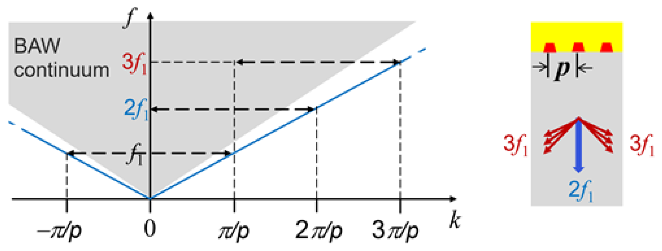
While $N^{\left(S\right)}$ and $N^{\left(D\right)}$ are real, the contribution $N^{\left(2H\right)}$ of the second harmonic is ordinarily complex due to radiation of the second harmonic into the bulk. We shall denote the real part of the total effective nonlinearity parameter N by N′ and its imaginary part by N″. In an infinite periodic system, bulk waves are radiated at the second harmonic frequency into the substrate with wave-vector vertical to the surface. The reason for their generation is explained in Figure 5. In an infinite periodic structure, the Bloch–Floquet exponent of the generalized displacement field, associated with the second harmonic of a Brillouin zone boundary excitation, is equal to zero in the reduced zone scheme. Consequently, it consists of bulk waves with wave-vectors vertical to the surface (blue arrow in the right subfigure of Figure 5). In the case of the third harmonic, the magnitude of the Bloch–Floquet exponent in the reduced zone scheme is equal to $\pi /p$. Therefore, the generalized displacement field associated with the third harmonic contains bulk waves with wave-vectors inclined to the surface normal (red arrows in the right subfigure of Figure 5). The inclination angles of these wave-vectors may be obtained from the sections of the (X₁,X₃)-plane and the corresponding sheets of the slowness surface of bulk waves in the substrate material.

Bulk-wave radiation at the second and third harmonic frequencies in a SAW resonator was verified experimentally in [49]. For an infinite periodic system, it may be shown in a way similar to the derivation of Equation (6.71) in [16] that the imaginary part of $N^{\left(2H\right)}$ is related to the power flow of the second harmonic away from the electrodes and that it must be positive. Unless the bottom of the substrate reflects the bulk waves at the second harmonic frequency back to the electrodes and their damping is negligible, the imaginary part of $N^{\left(2H\right)}$ is larger than zero. In

Table 1. Real part (N’) of coefficient N in the nonlinear term of Equation (41), and relative contributions of second harmonic (N^(2H)), static field (N^(S)) and third-order nonlinearity (N^(D)) to N. η: metallization ratio, f_r: resonance frequency. a: determined with generalized tensor S⁽³⁾ for LiNbO₃ that contains the contributions of the second-order and third-order elastic constants, while the FOECs were set equal to zero. b: determined with S⁽³⁾ = 0 for LiNbO₃.

N′ (a.u.)	N(2H)/N′	N(S)/N′	N(D)/N′	η	f᷊ (MHz)
6.21	−0.44 + 1.30i	−1.19	2.64	0.375	885	a
4.08	−0.81 + 2.13i	−1.68	3.48	0.5	875	a
3.09	−0.98 + 2.90i	−2.14	4.12	0.625	870	a
2.33	−1.11 + 3.46i	−2.84	4.95	0.75	869	a
7.04	−0.47 + 1.23i	−0.97	2.44	0.5	875	b

, the real part of the effective nonlinearity coefficient N and the relative sizes of the second harmonic contribution (both real and imaginary parts), of the static and of the direct contributions are provided for a TC-SAW system. The normalization

$$\underset{A}{\overset{}{{\displaystyle \iint }}}{U}_m^{\left(F\right)*}{\mathsf{\Delta }}_{mn}{U}_n^{\left(F\right)}d{\mathit{X}}_{1}d{\mathit{X}}_3=1$$

(56)

was chosen. The data show that there is a significant dependence of the nonlinearity coefficient on the metallization ratio. The direct contribution via the generalized tensor S⁽³⁾ plays a dominant role.

We note that the above considerations also apply to BAW resonators. For solidly mounted resonators with the piezoelectric layer between upper and lower electrode placed on a Bragg reflector, the coefficient N can acquire an imaginary part if the second harmonic of the linear resonance does not fall into a stop band of the Bragg reflector.

For frequencies in the neighborhood of the resonance frequency, the shape of the resonance curve and the phase response follows from (41). Inserting the stationary Ansatz $A\left(\tau \right)=A_0\exp \left(i\Omega \tau \right)$ in (41) yields a cubic equation in${\left|A_0\right|}^2$, which may be brought into the form

$$\Omega ==\pm \sqrt{\left({\left|F\right|}^2/{\left|A_0\right|}^2\right)-{\left(\mathsf{\gamma }+N^{″}{\left|A_0\right|}^2\right)}^2}+N^{\prime }{\left|A_0\right|}^2.$$

(57)

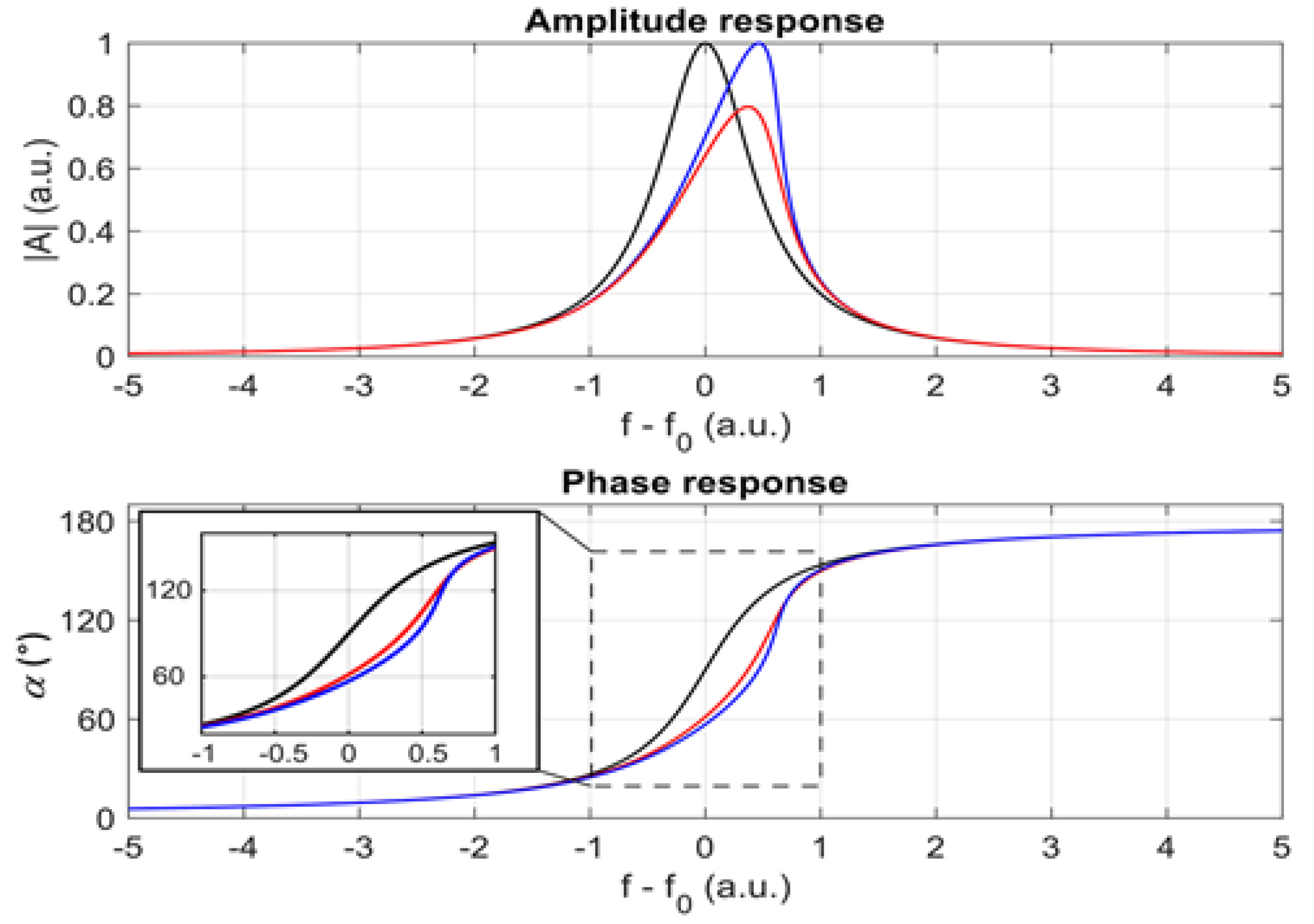
From (57), one readily deduces that the sign of the real part $N^{\prime }$ of the complex coefficient N decides on whether the resonance curve is inclined to negative ($N^{\prime }<0$) or positive ($N^{\prime }>0$) frequencies. The amplitude |A₀| reaches its maximum when the argument of the square root in (57) vanishes. Consequently, the presence of a positive imaginary part $N^{″}$ of N reduces this maximum in comparison to the linear case. The effect of the real and imaginary parts of N on the amplitude and phase response of a resonator is shown schematically in Figure 6.

The phase response of the resonator is affected by both real and imaginary parts of the coefficient N, too. Choosing F to be real and writing $A_0=\left|A_0\right|\exp \left(i\alpha \right)$, we obtain for the phase angle $\alpha$:

$$\tan \alpha =\left(\gamma +N^{″}{\left|A_0\right|}^2\right)/\left(\Omega -N^{\prime }{\left|A_0\right|}^2\right).$$

(58)

6. Reflection of Bulk Waves from the Bottom of the Substrate

As mentioned in the previous subsection, even an infinite periodic arrangement of electrodes generates bulk waves as part of second and third harmonics of fundamentals that are surface waves. If the bottom surface of the substrate is sufficiently smooth, these bulk waves undergo specular reflection, travel back to the upper surface and influence the current in the electrodes. This has been verified experimentally by Solal et al. [48]. In order to simulate this phenomenon, it is desirable to restrict computations to an area in the (X₁,X₃)-plane that is not larger in depth than the area used in FEM simulations of linear SAWs (h in Figure 7). However, in practice, the distance between the two surfaces of the sample (H in Figure 7) is much larger, H >> h. In order to bypass this problem, one can take advantage of the fact that below a certain depth, the generalized displacement field at the second-harmonic or third-harmonic frequency of a fundamental surface wave is approximately that of pure bulk waves, and apply an impedance boundary condition at the bottom of a simulation area of thickness h. This is demonstrated in the following for bulk wave radiation of the second harmonic frequency in a system with an infinite periodic arrangement of electrodes.

In this system, the generalized displacement field associated with the second harmonic, $\exp \left(2i{\omega }_{1}t\right)U_j^{\left(2H\right)}\left(X_1,X_3\right)+c.c.$, is a p-periodic function of X₁ and may therefore be written as a Fourier series,

$$U_j^{\left(2H\right)}\left(X_1,X_3\right)={\displaystyle \sum }_{n=-\infty }^{\infty }\left[e^{i2\pi n{\mathit{X}}_1/p} V_j^{\left(n\right)}\left({\mathit{X}}_3\right)\right].$$

(59)

In the substrate, the functions$V_j^{\left(n\right)}\left(X_3\right)$ are of the form

$$V_j^{\left(n\right)}\left(X_3\right)={\displaystyle \sum }_{r=1}^{N_r}{w}_j^{\left(n,r\right)} e^{i{q}^{\left(n,r\right)}\left({\mathit{X}}_3+h\right)} A^{\left(n,r\right)} +{\delta }_{n0}{\delta }_{j4}\left({\phi }_0+{\phi }_1\left({\mathit{X}}_3+h\right)\right)$$

(60)

with generalized four-component polarization vectors ${\mathit{w}}^{\left(n,r\right)}$, normalized in a suitable way, wave-vector components $q^{\left(n,r\right)}$ and coefficients $A^{\left(n,r\right)}, {\phi }_0, {\phi }_1$. For $n\ne 0$ the number $N_r$ of partial waves in the sum on the right-hand side of (60) is eight, while in the case $n=0$ it is equal to six. The polarization vectors and wave-vector components follow from the Christoffel equation for the substrate, extended to account for piezoelectricity. The coefficients $A^{\left(n,r\right)}, {\phi }_0, {\phi }_1$ are unknown.

Depending on the value of ${\omega }_1$, the functions $V_j^{\left(n\right)}\left(X_3\right)$ are localized at the surface, i.e., they decay exponentially into the substrate, or they contain plain wave components that radiate energy into the bulk of the substrate and from the bottom of the substrate back to the top surface. For frequencies ${\omega }_1/\left(2\pi \right)$ smaller or close to the resonance frequency, it is only the Fourier component n = 0 in (60) that contains bulk wave contributions. At the bottom of the substrate (X₃ = −H), boundary conditions must be specified. As an example, we require that the bottom surface is traction-free and the electric potential is zero. This yields the four equations

$$\begin{gathered} {\displaystyle \sum }_{r=1}^6{C}_{m3 k3}{w}_k^{\left(0,r\right)}\exp \left(i{q}^{\left(0,r\right)}\left(h-H\right)\right)i{q}^{\left(0,r\right)} A^{\left(0,r\right)}+C_{m3 43}{\phi }_1=0, \\ m=1,2,3, \end{gathered}$$

(61)

$${\displaystyle \sum }_{r=1}^6{w}_4^{\left(0,r\right)}\exp \left(i{q}^{\left(0,r\right)}\left(h-H\right)\right) A^{\left(0,r\right)}+{\phi }_0+{\phi }_1\left(h-H\right)=0$$

(62)

.

At ${\mathit{X}}_3=-h$, the generalized four-component displacement field of the second harmonic and its first derivative with respect to ${\mathit{X}}_3$ is continuous, which yields the eight equations

$$U_j^{\left(2H\right)}\left(X_1,-h\right)={{\displaystyle \sum }}_{r=1}^{N_r}{w}_j^{\left(0,r\right)} A^{\left(0,r\right)} +{\delta }_{j4}{\phi }_0,$$

(63)

$${\left[\frac{\partial }{\partial {\mathit{X}}_3}{U}_j^{\left(2H\right)}\left({\mathit{X}}_1,{\mathit{X}}_3\right)\right]}_{X_3=-h}={\displaystyle \sum }_{r=1}^{N_r}{w}_j^{\left(0,r\right)}i{q}^{\left(0,r\right)} A^{\left(0,r\right)} +{\delta }_{j4} {\phi }_1$$

(64)

for $j=1,\dots ,4$. The depth h was chosen to be sufficiently large, such that the X₁-dependence of ${\mathit{U}}^{\left(2H\right)}$ may be neglected. Solving (61)–(63) for eight variables $A^{\left(0,r\right)}, {\phi }_0, {\phi }_1$ and inserting this solution in (64) yields an effective boundary condition at X₃ = −h of the form

$${\left[\frac{\partial }{\partial {\mathit{X}}_3}{U}_j^{\left(2H\right)}\left({\mathit{X}}_1,{\mathit{X}}_3\right)\right]}_{X_3=-h}=M_{jk}\left(H-h\right) U_k^{\left(2H\right)}\left(X_1,-h\right)$$

(65)

with a frequency-dependent matrix M, which follows from the solution of a system of eight linear equations.

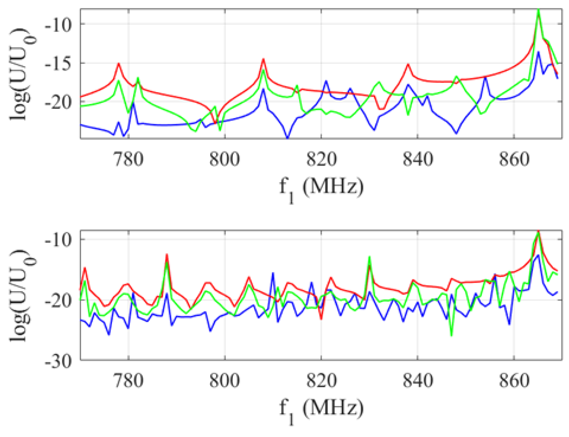
This procedure can be extended to Fourier components $n\ne 0$ in a straightforward way. Figure 8 shows the three components of the displacement field associated with the second harmonic at a fixed depth. They were computed with the boundary condition (65). For two different thicknesses of the substrate, typical Fabry–Perot type resonances are visible. For a rough estimate of the periodicity of the resonance peaks in the case of the displacement component U₃, one may argue as follows. The distance between neighboring frequencies of plate vibrations with displacements predominantly vertical to the surfaces is approximately v_L/(2L), where L is the thickness of the plate and v_L is the phase velocity of quasi-longitudinal bulk waves with wave vector vertical to the surfaces of the plate. In the plots of the displacement field associated with the second harmonic as a function of the fundamental frequency f₁, we therefore expect a distance Δf₁ $\approx$ v_L/(4H) between neighboring resonance peaks of the same kind for the displacement component U₃. With the velocity of quasi-longitudinal waves in the substrate (LiNbO₃-rot128YX) with wave-vector in the X₃-direction v_L = 7091 m/s, we expect Δf₁ ≈ 30 MHz for H = 59.24 µm and Δf₁ ≈ 8.5 MHz for H = 209.24 µm. This corresponds well with the data in Figure 8. The reflected quasi-transverse waves, polarized predominantly in the X₂-direction, and purely transverse waves, polarized in the X₁-direction, together with the quasi-longitudinal waves give rise to complex interference patterns, since all three components are coupled in the spatial domain close to the surface.

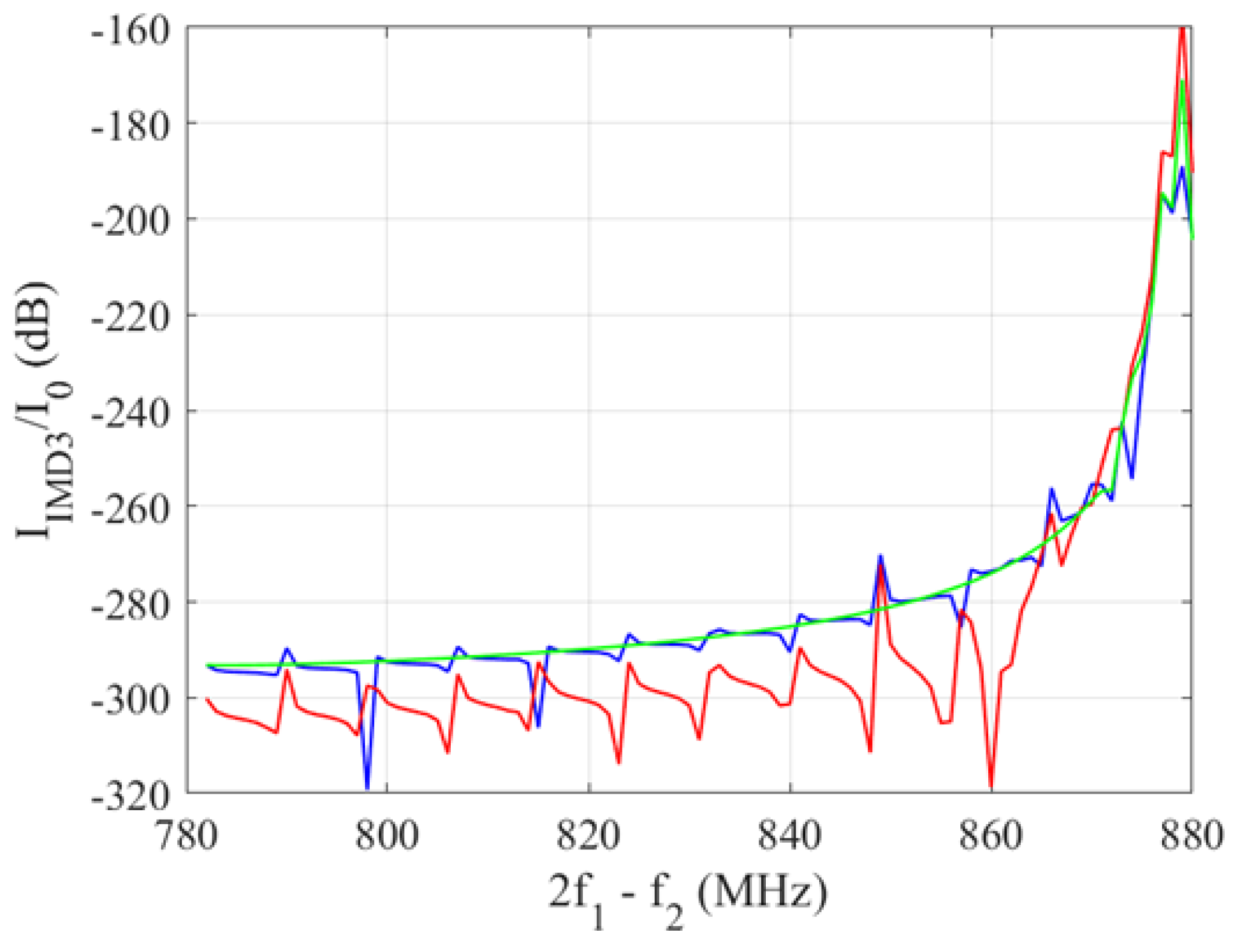
The Fabry–Perot resonances in the generalized displacement field of the second harmonic influences the IMD3 current as shown in Figure 9.

At frequencies f₁ much larger than the resonance frequency, where terms of the Fourier series (59) with $n\ne 0$ are not localized at the surface, the corresponding bulk waves propagate away from the surface at an angle different from 90°. After being reflected at the bottom of the substrate, they will travel back and reach the top surface outside the area covered by electrodes in the case of a finite device. Nevertheless, they may influence the IMD3 current in this device.

7. Recursive Procedure for Finite, Truncated Periodic Systems

In this section, a method is presented for an efficient calculation of the nonlinearly generated fields and currents for a system consisting of a periodically arranged, but finite number of electrodes (Figure 1b). In the case of third-order intermodulations, this concerns the fields ${\mathit{U}}^{\left(\mathbf{2}\mathit{H}\right)}, {\mathit{U}}^{\left(\mathit{L}\mathit{F}\right)}, U^{\left(\mathit{I}\mathit{M}\mathbf{3}\right)}$ and the IMD3 current. The basic task is to numerically solve the inhomogeneous systems of linear Equations (9), (12), (13) and (15) with the structure of the matrix $\tilde{\mathit{M}}\left(\omega \right)$ and the inhomogeneities (right-hand sides of the linear equations) resulting from the geometry of the system.

Recently, Koskela and Plessky [50,51] introduced a method for the FEM calculation of linear fields and admittances in such systems, which leads to an enormous reduction of computing time as compared to the standard FEM approach. This method is based on the elimination of the internal degrees of freedom in a unit cell via the Schur complement and the principle of cascading, well-known in P-matrix theory [52]. For the computations of nonlinear fields within the perturbation scheme used here, cascading is not directly applicable. This is because the inhomogeneities differ between different cells unlike the linear case, where the inhomogeneities result from the electrodes’ electric potential and, consequently, there are only two different cell inhomogeneities.

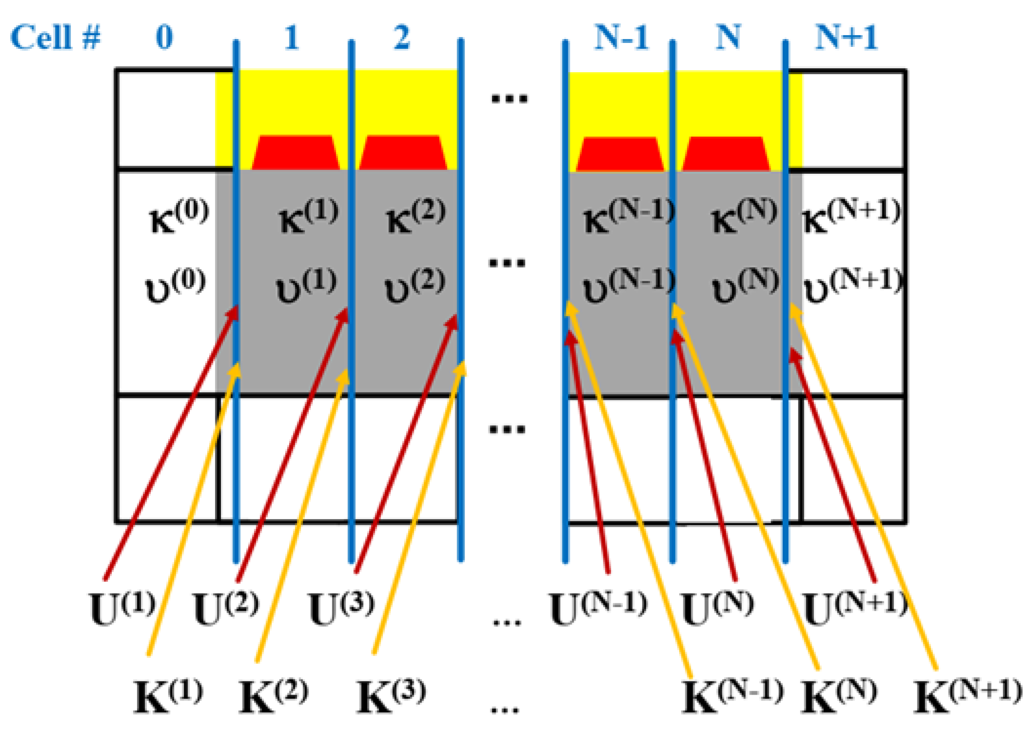
Here, we present a simple scheme which makes use of recursion relations and which is described in the following. It is applied to the system shown in Figure 10, which is divided in N + 2 cells, N of them being identical. The mesh is chosen such that no boundary between neighboring cells divides a finite element into two parts. In addition, we impose the following requirements on the arrangement of the mesh. The finite elements on the left side of a boundary between two neighboring cells (blue vertical line in Figure 10), having common nodes with this boundary, form a vertical layer. We require that these vertical layers are identical in the cells with numbers 0 to N. Likewise, the vertical layers of finite elements on the right of a boundary having common nodes with this boundary are identical in the cells with numbers 1 to N + 1. These additional requirements to the mesh are not essential, but simplify the calculations. The sub-meshes in the cells 1 to N are identical.

7.1. Derivation of the Recursion Relation

The systems of linear Equations (9), (12), (13) and (15) are of the general form

$${\displaystyle \sum }_{{\mathsf{\ell }}^{\prime }}{M}_{j{j}^{\prime }}^{\left(\mathsf{\ell }{\mathsf{\ell }}^{\prime }\right)}\left(\omega \right) {\widehat{U}}_{j^{\prime }}^{\left({\mathsf{\ell }}^{\prime }\right)}={\widehat{K}}_j^{(\mathsf{\ell })}.$$

(66)

We now introduce a cell index n and group the degrees of freedom ${\widehat{U}}_j^{(\mathsf{\ell })}$ on nodes $\mathsf{\ell }$ in the interior of the n-th cell in a column vector ${\mathit{\upsilon }}^{\left(n\right)}$. The degrees of freedom ${\widehat{U}}_j^{(\mathsf{\ell })}$ on nodes $\ell$, which are situated on the boundary between the n-th and (n−1)-th cell, are grouped in a column vector ${\mathit{U}}^{\left(n\right)}$. In the same way, with the quantities ${\widehat{K}}_j^{(\mathsf{\ell })}$ on the right-hand side of (66) with node number $\mathsf{\ell }$ referring to the interior of the n-th cell, a column vector ${\mathit{\kappa }}^{\left(n\right)}$ is formed. The quantities ${\widehat{K}}_j^{(\mathsf{\ell })}$ with node number $\mathsf{\ell }$ referring to the boundary between the n-th and (n−1)-th cell form the column vector ${\mathit{K}}^{\left(n\right)}$.

The interior degrees of freedom may be eliminated by using the following relation:

$${\mathit{M}}^{\left(n,ii\right)}{\mathit{\upsilon }}^{\left(n\right)}={\mathit{\kappa }}^{\left(n\right)}-{\mathit{M}}^{\left(n,i<\right)}{\mathit{U}}^{\left(n-1\right)}-{\mathit{M}}^{\left(n,i>\right)}{\mathit{U}}^{\left(n\right)}$$

(67)

for n = 1,…, N. For n = 0, the second term on the right-hand side and for n = N + 1 the third term on the right-hand side of (67) is absent. ${\mathit{M}}^{\left(n,ii\right)}, {\mathit{M}}^{\left(n,i<\right)}, {\mathit{M}}^{\left(n,i>\right)}$ are submatrices of the coefficient matrix on the left-hand side of (66) with the left node index $\mathsf{\ell }$of its matrix elements ${\mathit{M}}_{j{j}^{\prime }}^{\left(\mathsf{\ell }{\mathsf{\ell }}^{\prime }\right)}\left(\omega \right)$ referring to all nodes in the interior of the n-th cell. The matrix elements of ${\mathit{M}}^{\left(n,ii\right)}$ connect two nodes in the interior of cell n (these two nodes may be identical). The right node indices of the matrix elements of ${\mathit{M}}^{\left(n,i<\right)}$ (${\mathit{M}}^{\left(n,i>\right)}$) refer to nodes on the left (right) boundary of cell n.

The system of Equation (67) is solved for ${\mathit{\upsilon }}^{\left(n\right)}$ and the result is inserted in

$${\mathit{M}}^{\left(n,<i\right)}{\mathit{\upsilon }}^{\left(n\right)}+{\mathit{M}}^{\left(n-1,>i\right)}{\mathit{\upsilon }}^{\left(n-1\right)}={\mathit{K}}^{\left(n\right)}-{\mathit{M}}^{\left(n,<<\right)}{\mathit{U}}^{\left(n\right)}$$

(68)

for n = 1,…, N + 1, where ${\mathit{M}}^{\left(n,<i\right)}, {\mathit{M}}^{\left(n,>i\right)}, {\mathit{M}}^{\left(n,<<\right)}$ are submatrices of the coefficient matrix in (66). The right node indices of ${\mathit{M}}^{\left(n,<i\right)}$ and ${\mathit{M}}^{\left(n,>i\right)}$ refer to nodes in the interior of cell n. The left node indices of the matrix elements of ${\mathit{M}}^{\left(n,<i\right)}$ (${\mathit{M}}^{\left(n,>i\right)}$) refer to nodes on the left (right) boundary of cell n, whereas the matrix elements of ${\mathit{M}}^{\left(n,<<\right)}$ connect two (possibly identical) nodes on the left boundary of cell n.

We note that with the conditions we have imposed on the mesh, the matrices ${\mathit{M}}^{\left(n,ii\right)}, {\mathit{M}}^{\left(n,i<\right)}, {\mathit{M}}^{\left(n,i>\right)}, {\mathit{M}}^{\left(n,<i\right)}, {\mathit{M}}^{\left(n,>i\right)}, {\mathit{M}}^{\left(n,<<\right)}$ are independent of the cell number n for the cells 1 to N. In addition, ${\mathit{M}}^{\left(N+1,<<\right)}={\mathit{M}}^{\left(N,<<\right)}$. Therefore, we shall drop the cell number in the notation of these matrices and keep this number only in ${\mathit{M}}^{\left(0,ii\right)}, {\mathit{M}}^{\left(N+1,ii\right)}, {\mathit{M}}^{\left(0,i>\right)}, {\mathit{M}}^{\left(N+1,i<\right)}, {\mathit{M}}^{\left(0,>i\right)}, {\mathit{M}}^{\left(N+1,<i\right)}$.

Having eliminated ${\upsilon }^{\left(n\right)}$, n = 0,…, N + 1, the following recursion relation results for the vectors ${\mathit{U}}^{\left(n\right)}$,

$$\mathit{A}{\mathit{U}}^{\left(n-1\right)}+\mathit{B}{\mathit{U}}^{\left(n\right)}+\mathit{C}{\mathit{U}}^{\left(n+1\right)}={\mathit{J}}^{\left(n\right)},$$

(69)

for n = 2,…, N. Furthermore

$${\mathit{B}}^{\left(0\right)}{\mathit{U}}^{\left(1\right)}+\mathit{C}{\mathit{U}}^{\left(2\right)}={\mathit{J}}^{\left(1\right)},$$

(70)

$$\mathit{A}{\mathit{U}}^{\left(N\right)}+{\mathit{B}}^{\left(N+1\right)}{\mathit{U}}^{\left(N+1\right)}={\mathit{J}}^{\left(N+1\right)}.$$

(71)

The matrices $\mathit{A}, \mathit{B}, \mathit{C}, {\mathit{B}}^{\left(0\right)}, {\mathit{B}}^{\left(N+1\right)}$ are related to the quantities introduced before via

$$\mathit{A}=-{\mathit{M}}^{\left(>i\right)}{\mathit{M}}^{\left(ii\right)-1} {\mathit{M}}^{\left(i<\right)},$$

(72)

$$\mathit{B}=-{\mathit{M}}^{\left(>i\right)}{\mathit{M}}^{\left(ii\right)-1} {\mathit{M}}^{\left(i>\right)}-{\mathit{M}}^{\left(<i\right)}{\mathit{M}}^{\left(ii\right)-1} {\mathit{M}}^{\left(i<\right)}+{\mathit{M}}^{(\ll )},$$

(73)

$$\mathit{C}=-{\mathit{M}}^{\left(<i\right)}{\mathit{M}}^{\left(ii\right)-1} {\mathit{M}}^{\left(i>\right)},$$

(74)

$${\mathit{B}}^{\left(0\right)}=-{\mathit{M}}^{\left(0,>i\right)}{\mathit{M}}^{\left(0,ii\right)-1} {\mathit{M}}^{\left(0,i>\right)}-{\mathit{M}}^{\left(<i\right)}{\mathit{M}}^{\left(ii\right)-1} {\mathit{M}}^{\left(i<\right)}+{\mathit{M}}^{(\ll )},$$

(75)

$${\mathit{B}}^{\left(N+1\right)}=-{\mathit{M}}^{\left(>i\right)}{\mathit{M}}^{\left(ii\right)-1} {\mathit{M}}^{\left(i>\right)}-{\mathit{M}}^{\left(N+1,<i\right)}{\mathit{M}}^{\left(N+1,ii\right)-1} {\mathit{M}}^{\left(N+1,i<\right)}+{\mathit{M}}^{(\ll )}.$$

(76)

The column vectors ${\mathbf{J}}^{\left(n\right)}, n=1,\dots ,N$, are defined as:

$${\mathit{J}}^{\left(n\right)}=-{\mathit{M}}^{\left(>i\right)}{\mathit{M}}^{\left(ii\right)-1} {\mathit{\kappa }}^{\left(n-1\right)}-{\mathit{M}}^{\left(<i\right)}{\mathit{M}}^{\left(ii\right)-1} {\mathit{\kappa }}^{\left(n\right)}+{\mathit{K}}^{\left(n\right)},$$

(77)

and

$${\mathit{J}}^{\left(1\right)}=-{\mathit{M}}^{\left(0,>i\right)}{\mathit{M}}^{\left(0,ii\right)-1} {\mathit{\kappa }}^{\left(0\right)}-{\mathit{M}}^{\left(<i\right)}{\mathit{M}}^{\left(ii\right)-1} {\mathit{\kappa }}^{\left(1\right)}+{\mathit{K}}^{\left(1\right)},$$

(78)

$${\mathit{J}}^{\left(N+1\right)}=-{\mathit{M}}^{\left(>i\right)}{\mathit{M}}^{\left(ii\right)-1} {\mathit{\kappa }}^{\left(N\right)}-{\mathit{M}}^{\left(N+1,<i\right)}{M}^{\left(N+1,ii\right)-1} {\mathit{\kappa }}^{\left(N+1\right)}+{\mathit{K}}^{\left(N+1\right)}.$$

(79)

From (69)–(71), the degrees of freedom on the cell boundaries, ${\mathit{U}}^{\left(n\right)}, n=1,\dots ,N+1$, are determined in the following way.

First, we compute matrices ${\widehat{\mathit{B}}}_n, n=1,\dots ,N-1$, and vectors ${\widehat{\mathit{J}}}_n, n=1,\dots ,N$, recursively via

$${\widehat{\mathit{B}}}_n=\mathit{B}-\mathit{A} {\widehat{\mathit{B}}}_{n-1}^{-1}\mathit{C},$$

(80)

$${\widehat{\mathit{J}}}_{n+1}={\mathit{J}}^{\left(n+1\right)}-\mathit{A} {\widehat{\mathit{B}}}_{n-1}^{-1}{\widehat{\mathit{J}}}_n,$$

(81)

starting the recursions with

$${\widehat{\mathit{B}}}_0={\mathit{B}}^{\left(0\right)},$$

(82)

$${\widehat{\mathit{J}}}_1={\mathit{J}}^{\left(1\right)},$$

(83)

and defining

$${\widehat{\mathit{B}}}_N={\mathit{B}}^{\left(N+1\right)}-A {\widehat{\mathit{B}}}_{N-1}^{-1}\mathit{C}.$$

(84)

With the help of these matrices and vectors, which have been stored, the vectors ${\mathit{U}}^{\left(n\right)}, n=1,\dots ,N+1$ are subsequently computed by making use of the following downwards recursion:

$${\mathit{U}}^{\left(n\right)}={\widehat{\mathit{B}}}_{n-1}^{-1} \left({\widehat{\mathit{J}}}_n-\mathit{C}{\mathit{U}}^{\left(n+1\right)}\right),$$

(85)

for $n=N,\dots ,1$, and starting with

$${\mathit{U}}^{\left(N+1\right)}={\widehat{\mathit{B}}}_N^{-1} {\widehat{\mathit{J}}}_{N+1}.$$

(86)

7.2. Results for IMD2 Displacements

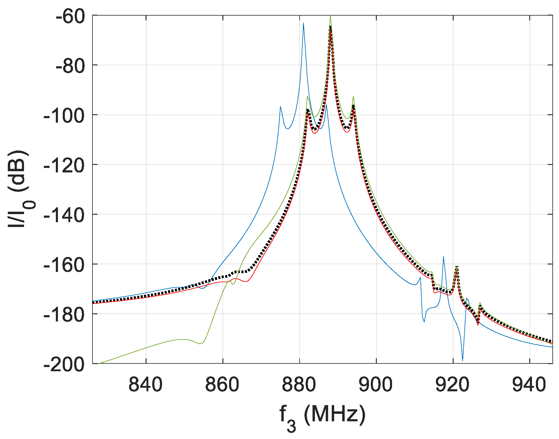
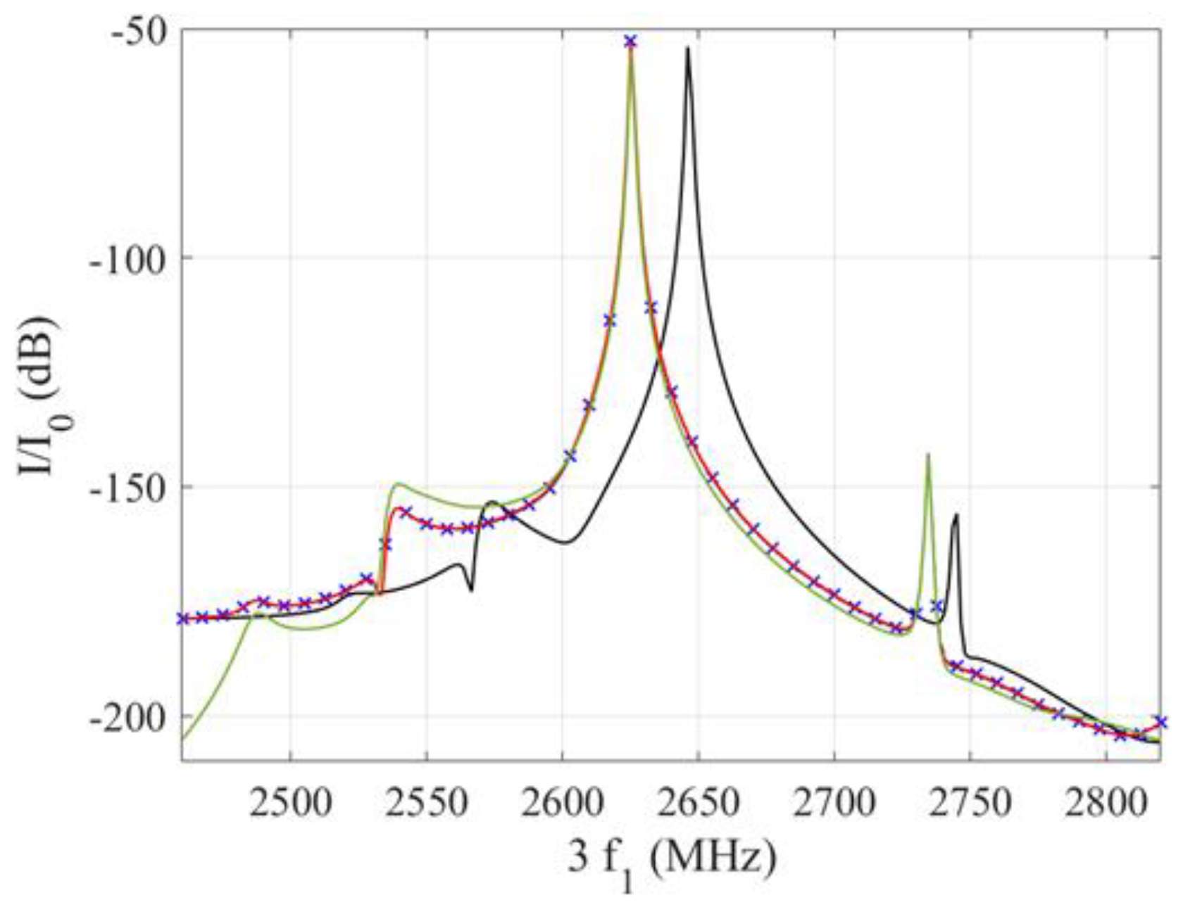
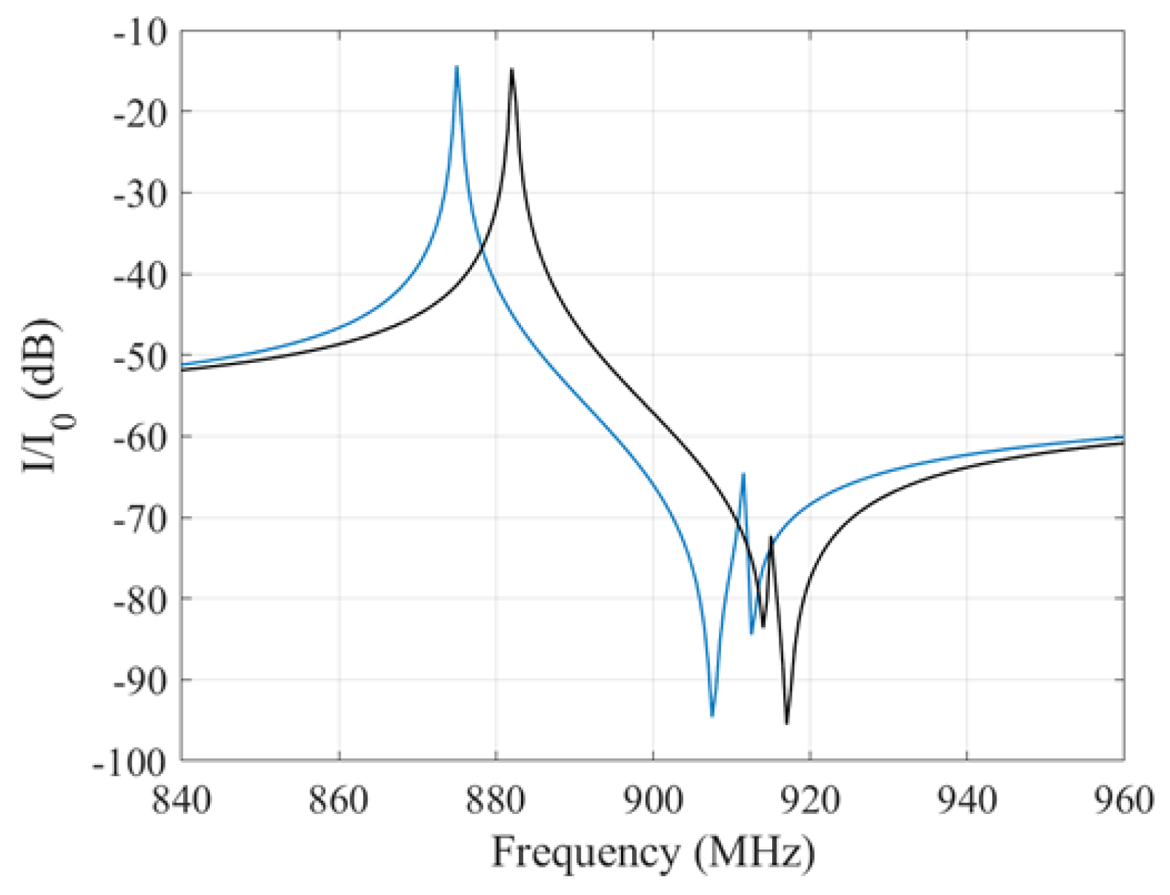
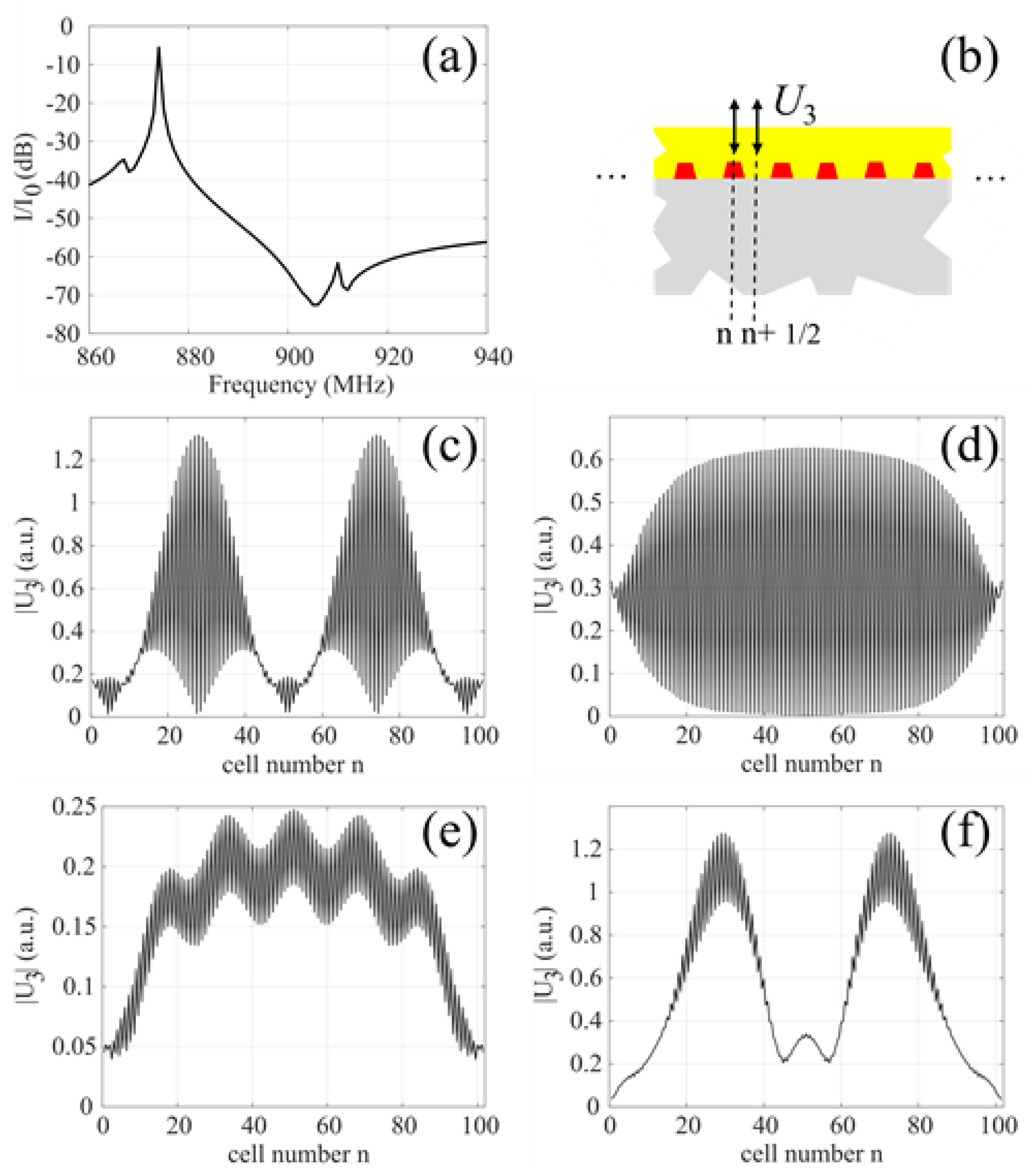
The recursion scheme outlined in the previous subsection has been implemented for the computation of displacements and electrical currents, generated by second-order nonlinearity, in TC-SAW systems consisting of finite numbers of electrodes. In Figure 11, results are shown for the displacements at the surface of the SiO₂ film at positions above the centers of the electrodes and halfway between the surface points above the centers of neighboring electrodes (Figure 11b). The pitch, metallization ratio, electrode height and film thickness were the same as those in the infinite periodic system that Figure 2, Figure 3 and Figure 4 refer to. The linear admittance of this system is shown in Figure 11a. The displacement patterns for two input frequencies as linear response to a periodic electric potential of $\pm$1 V (peak value) are shown in Figure 11c,d. The input frequency f₁ (=860 MHz) is about 14 MHz below, and f₂ (=890 MHz) about 16 MHz above the resonance frequency. Figure 11e shows the displacement pattern for the second harmonic (H2) of the input tone f₂. It varies more strongly along the length of the device than the displacement associated with its fundamental (Figure 11d). The displacement pattern of the second order intermodulation (IMD2) at frequency f₁ + f₂, is shown in Figure 11f. Similar to the pattern associated with the input tone f₁ (Figure 11c), the displacements in the center of the device are small as compared to those near the 30th and 70th cells.

8. Conclusions

In summary, a perturbation-theoretical approach, based on nonlinear electro-elasticity theory and the finite element method, has been presented, which allows for calculations of quantities in SAW devices generated by second-order and third-order nonlinearity. These include displacements and electric fields as well as electrical currents associated with intermodulations of second and third order, second and third harmonic generation and the dependence of the resonance curve and phase response of a SAW resonator on input voltage. The FEM approach works with two-dimensional elements, but fully accounts for all three Cartesian components of the mechanical and electric displacement field. Infinite periodic as well as finite systems with spatial periodicities can be treated. The application of perturbation theory is justified by the smallness of typical strains occurring in SAW devices. It leads to a hierarchy of linear boundary value problems. By this approach, complex systems become accessible to numerical simulations of nonlinear effects, which would be hard to deal with by numerical schemes solving directly nonlinear partial differential equations.

A major goal of our approach was to enable computations of third-order intermodulations on a laptop computer. This opens the possibility for the designer of SAW devices to minimize undesired nonlinear effects with the help of simulations, which can be carried out with reasonable numerical effort and which are directly based on material properties. For this purpose, algorithms were developed that increase the efficiency of certain parts of the computations. These include an alternative way of calculating IMD2 and IMD3 currents in the electrodes via overlap integrals, which avoid the computation of the IMD2/IMD3 field. In addition, an impedance boundary condition is presented to account for reflections of bulk waves from the bottom of a thick substrate and, in particular, a recursive algorithm for finite periodic systems which is related to the cascading method introduced by Koskela and Plessky for FEM computations of linear quantities in SAW devices [50,51].

The recursive scheme, introduced here in the context of electro-elastic nonlinearity, may also be applied to simulations of thermal effects in SAW devices to reduce computational effort; for example, the effect of intrinsic heating on the resonance frequency, giving rise to additional nonlinearity (e.g., [53] for the case of BAW resonators). The variation of the temperature field between different unit cells of the interdigital transducers or reflectors precludes cascading, but still allows for application of the recursive algorithm.

Prerequisite of quantitative simulations of nonlinear effects is the availability of reliable nonlinear material constants up to fourth order for all materials that fill those parts of the SAW device where comparatively large strains or electric fields occur. In the case of thin films, the required material constants may differ from those of the corresponding bulk material and may depend on details of the fabrication process.

References

1. Inoue, S.; Mitobe, S.; Hara, M.; Iwaki, M.; Tsutsumi, J.; Nakamura, H.; Ueda, M.; Satoh, Y. A precise nonlinear simulation for SAW duplexers considering nonlinear elasticity. In Proceedings of the 41st European Microwave Conference, Manchester, UK, 10–13 October 2011; pp. 599–602. [Google Scholar]
2. Inoue, S.; Hara, M.; Iwaki, M.; Tsutsumi, J.; Nakamura, H.; Ueda, M.; Satoh, Y.; Mitobe, S. A nonlinear elastic model for predicting triple beat in SAW duplexers. In Proceedings of the 2011 IEEE International Ultrasonics Symposium, Orlando, FL, USA, 18–21 October 2011; pp. 1837–1841. [Google Scholar]
3. Nakagawa, R.; Suzuki, T.; Shimizu, H.; Kyoya, H.; Katsuhiro, N. A new simulation method for nonlinear characteristics of SAW devices. In Proceedings of the IEEE European Microwave Integrated Circuit Conference, Nuremberg, Germany, 6–8 October 2013; pp. 292–295. [Google Scholar]
4. Mayer, M.; Ruile, W.; Johnson, J.; Bleyl, I.; Wagner, K.; Mayer, A.; Mayer, E. Rigorous COM and P-matrix approaches to the simulation of third-order intermodulation distortion and triple beat in SAW filters. In Proceedings of the 2013 IEEE International Ultrasonics Symposium, Prague, Czech Republic, 21–25 July 2013; pp. 1965–1968. [Google Scholar]
5. González-Rodríguez, M.; Collado, C.; Mateu, J.; Gonzalez-Arbesú, J.M.; Huebner, S.; Aigner, R. Fast simulation method of distributed nonlinearities in surface acoustic wave resonators. In Proceedings of the 2020 IEEE International Ultrasonics Symposium, Las Vegas, NV, USA, 7–11 September 2020. [Google Scholar]
6. Shim, D.S.; Feld, D.A. A general nonlinear Mason model of arbitrary nonlinearities in a piezoelectric film. In Proceedings of the 2010 IEEE International Ultrasonics Symposium, San Diego, CA, USA, 11–14 October 2010; pp. 295–300. [Google Scholar]
7. Feld, D.A.; Shim, D.S.; Fouladi, S.; Bayatpur, F. Advances in nonlinear measurement & modeling of bulk acoustic wave resonators (invited). In Proceedings of the 2014 IEEE International Ultrasonics Symposium, 3–6 September 2014; pp. 264–272. [Google Scholar]
8. Mayer, A.; Mayer, E.; Mayer, M.; Jäger, P.; Ruile, W.; Bleyl, I.; Wagner, K. Effective nonlinear constants for SAW devices from FEM calculations. In Proceedings of the 2015 IEEE International Ultrasonics Symposium, Taipei, Taiwan, 21–24 October 2015. [Google Scholar]
9. Mayer, A.; Mayer, E.; Mayer, M.; Jäger, P.; Ruile, W.; Bleyl, I.; Wagner, K. Full 2D-FEM calculations of third-order intermodulations in SAW devices. In Proceedings of the 2016 IEEE International Ultrasonics Symposium, Tours, France, 18–21 September 2016. [Google Scholar]
10. Chauhan, V.; Mayer, M.; Mayer, E.; Ruile, W.; Ebner, T.; Bleyl, I.; Wagner, K.C.; Weigel, R.; Mayer, A.P.; Hagelauer, A. Investigation on third-order intermodulation distortions due to material nonlinearities in TC-SAW devices. IEEE Trans. Ultrason. Ferroelectr. Freq. Control 2018, 65, 1914–1924. [Google Scholar] [CrossRef]
11. Pang, X.; Yong, Y.-K. Novel FEM models of intermodulation effects in BAW and SAW devices. In Proceedings of the 2019 IEEE International Ultrasonics Symposium, 6–9 October 2019; pp. 177–180. [Google Scholar]
12. Pang, X.; Yong, Y.-K. Simulation of nonlinear resonance, amplitude-frequency, and harmonic generation effects in SAW and BAW devices. IEEE Trans. Ultrason. Ferroelectr. Freq. Control 2020, 67, 422–430. [Google Scholar] [CrossRef] [PubMed]
13. Guan, P.; Shi, R.C.; Yang, Y.; Han, T. Nonlinear analysis of temperature-compensated surface acoustic wave resonators. Sci. Sin.-Phys. Mech. Astron. 2021, 46, 123456. [Google Scholar] [CrossRef]
14. Guan, P.; Shi, R.; Yang, Y.; Qin, P.; Han, T. Mechanisms of third-order harmonic in TC-SAW resonators using a nonlinear FEM model. In Proceedings of the 2021 IEEE International Ultrasonics Symposium, Xi’an, China, 11–16 September 2021. [Google Scholar]
15. Forster, T.; Chauhan, V.; Mayer, M.; Mayer, E.; Mayer, A.; Ebner, T.; Wagner, K.; Hagelauer, A. Finite element simulations for predicting nonlinear responses of layered SAW systems. In Proceedings of the 2021 IEEE International Ultrasonics Symposium, Xi’an, China, 11–16 September 2021. [Google Scholar]
16. Mayer, A.P. Surface acoustic waves in nonlinear elastic media. Phys. Rep. 1995, 256, 237–366. [Google Scholar] [CrossRef]
17. Graßl, H.P.; Reindl, L.M.; Wörz, H.-W. State-of-the-art elastic SAW convolvers. In Recent Developments in Surface Acoustic Waves; Parker, D.F., Maugin, G.A., Eds.; Springer: Berlin/Heidelberg, Germany, 1988; pp. 2–13. [Google Scholar]
18. Campbell, C.K. Surface Acoustic Wave Devices for Mobile and Wireless Communications; Academic Press: San Diego, CA, USA, 1998; Chapter 17. [Google Scholar]
19. Matlack, K.H.; Kim, J.Y.; Jacobs, L.J.; Qu, J. Review of second harmonic generation measurement techniques for material state determination in metals, J. Nondestruct. Eval. 2015, 34, 273. [Google Scholar] [CrossRef]
20. Nelson, D.F. Electric, Optic and Acoustic Interactions in Dielectrics; Wiley: New York, NY, USA, 1979; Chapters 3 and 17. [Google Scholar]
21. Tiersten, H.F.; Baumhauer, J.C. Second harmonic generation and parametric excitation of surface waves in elastic and piezoelectric solids. J. Appl. Phys. 1974, 45, 4272–4287. [Google Scholar] [CrossRef]
22. Tiersten, H.F.; Baumhauer, J.C. An analysis of second harmonic generation of surface waves in piezoelectric solids. J. Appl. Phys. 1985, 58, 1867–1875. [Google Scholar] [CrossRef]
23. Maugin, G.A. ; Nonlinear Electromechanical Effects and Applications; World Scientific: Singapore, 1985. [Google Scholar]
24. Reutov, V.P. Use of the averaged variational principle for describing multiwave interactions of elastic surface waves. Radiophys. Quantum Electron. 1973, 16, 1307–1316. [Google Scholar] [CrossRef]
25. Parker, D.F.; David, E.A. Nonlinear piezoelectric surface waves. Int. J. Engng. Sci. 1989, 27, 565–581. [Google Scholar] [CrossRef]
26. Harvey, A.P.; Tupholme, G.E. Nonlinear mode coupling of two co-directional surface acoustic waves on a piezoelectric solid, Int. J. Engng. Sci. 1991, 29, 987–998. [Google Scholar] [CrossRef]
27. Tupholme, G.E.; Harvey, A.P. Intermodulation distortion of nonlinear piezoelectric surface waves. J. Mech. Phys. Solids 1992, 40, 1651–1661. [Google Scholar] [CrossRef]
28. Taylor, D.B.; Crampin, S. Surface waves in anisotropic media: Propagation in a homogeneous piezoelectric halfspace. Proc. Roy. Soc. London 1978, A364, 161–179. [Google Scholar]
29. Tupholme, G.E. Multiple scale techniques applied to nonlinear elastic and piezoelectric surface waves. In Recent Developments in Surface Acoustic Waves; Parker, D.F., Maugin, G.A., Eds.; Springer: Berlin/Heidelberg, Germany, 1988; pp. 14–20. [Google Scholar]
30. David, E.A.; Parker, D.F. Nonlinear evolution of piezoelectric SAWs. In Recent Developments in Surface Acoustic Waves; Parker, D.F., Maugin, G.A., Eds.; Springer: Berlin/Heidelberg, Germany, 1988; pp. 21–29. [Google Scholar]
31. Harvey, A.P.; Craine, R.E.; Syngellakis, S. Nonlinear piezoelectric surface acoustic waves using the multiple scales technique. In Recent Developments in Surface Acoustic Waves; Parker, D.F., Maugin, G.A., Eds.; Springer: Berlin/Heidelberg, Germany, 1988; pp. 30–35. [Google Scholar]
32. Tupholme, G.E.; Harvey, A.P. Nonlinear surface acoustic waves on a piezoelectric solid. Int. J. Engng. Sci. 1988, 26, 1161–1168. [Google Scholar] [CrossRef]
33. Tiersten, H.F. Linear Piezoelectric Plate Vibrations; Plenum Press: New York, NY, USA, 1969; Chapter 6. [Google Scholar]
34. Leibfried, G.; Ludwig, W. Gleichgewichtsbedingungen in der Gittertheorie. Z. Für Phys. 1960, 160, 80–92, [in German]. [Google Scholar] [CrossRef]
35. Cho, Y.; Yamanouchi, K. Nonlinear, elastic, piezoelectric, electrostrictive, and dielectric constants of LiNbO3. J. Appl. Phys. 1987, 61, 875–887. [Google Scholar] [CrossRef]
36. Kovacs, G.; Anhorn, M.; Engan, H.E.; Visintini, G.; Ruppel, C.C.W. Improved material constants for LiNbO3 and LiTaO3. In Proceedings of the IEEE Symposium on Ultrasonics, Honolulu, HI, USA, 4–7 December 1990; pp. 435–438. [Google Scholar]
37. Knapp, M.; Lomonosov, A.M.; Warkentin, P.; Jäger, P.M.; Ruile, W.; Kirschner, H.-P.; Honal, M.; Bleyl, I.; Mayer, A.P.; Reindl, L.M. Accurate characterization of SiO2 thin films using surface acoustic waves. IEEE Trans. Ultrason. Ferroelectr. Freq. Control 2015, 62, 736–743. [Google Scholar] [CrossRef]
38. Bogardus, E.H. Third-order elastic constants of Ge, MgO, and fused SiO2. J. Appl. Phys. 1965, 36, 2504–2513. [Google Scholar] [CrossRef]
39. Yost, W.T.; Breazeale, M.A. Adiabatic third-order elastic constants of fused silica. J. Appl. Phys. 1973, 44, 1909–1910. [Google Scholar] [CrossRef]
40. Kondo, K.; Lio, S.; Sawaoka, A. Nonlinear pressure dependence of the elastic moduli of fused quartz up to 3 GPa. J. Appl. Phys. 1981, 52, 754–758. [Google Scholar] [CrossRef]
41. Wang, H.; Li, M. Ab initio calculations of second-, third-, and fourth-order elastic constants for single crystals. Phys. Rev. B 2009, 79, 224102. [Google Scholar] [CrossRef]
42. Lubarda, V.A. New estimates of the third-order elastic constants for isotropic aggregates of cubic crystals. J. Mech. Phys. Solids 1997, 45, 471–490. [Google Scholar] [CrossRef]
43. Kube, C.M.; Arguelles, A.; Turner, J.A. On the acoustoelasticity of polycrystalline materials. J. Acoust. Soc. Am. 2015, 138, 1498–1507. [Google Scholar] [CrossRef] [PubMed]
44. Logan, D.L. A First Course in the Finite Element Method, 4th ed.; Thomson: Toronto, Canada, 2007; chapter 10. [Google Scholar]
45. Mayer, M.; Zaglmayr, S.; Wagner, K.; Schöberl, J. Perfectly matched layer finite element simulation of parasitic acoustic wave radiation in microacoustic devices. In Proceedings of the 2007 IEEE Ultrasonics Symposium Proceedings, New York, NY, USA, 28–31 October 2007; pp. 702–706. [Google Scholar]
46. Korsch, H.J.; Jodl, H.-J.; Hartmann, T. Chaos; Springer: Berlin/Heidelberg, Germany, 2008; chapter 8. [Google Scholar]
47. Nayfeh, A.H. Introduction to Perturbation Techniques; Wiley-VCH: Weinheim, Germany, 2004. [Google Scholar]
48. Parker, D.F.; Mayer, A.P.; Maradudin, A.A. The projection method for nonlinear surface acoustic waves. Wave Motion 1992, 16, 151–162. [Google Scholar] [CrossRef]
49. Solal, M.; Kokkonen, K.; Inoue, S.; Briot, J.-B.; Abbott, B.P.; Gamble, K.J. Observation of nonlinear harmonic generation of bulk modes in SAW devices. IEEE Trans. Ultrason., Ferroelectr., Freq. Control 2017, 64, 1361–1367. [Google Scholar] [CrossRef]
50. Koskela, J.; Maniadis, P.; Willemsen, B.A.; Turner, P.J.; Hammond, R.B.; Fenzi, N.O.; Plessky, V. Hierarchical cascading in 2D FEM simulation of finite SAW devices with periodic block structure. In Proceedings of the 2016 IEEE International Ultrasonics Symposium, Tours, France, 18–21 September 2016. [Google Scholar]
51. Koskela, J.; Plessky, V.; Willemsen, B.; Turner, P.; Hammond, B.; Fenzi, N. Hierarchical cascading algorithm for 2-D FEM simulation of finite SAW devices. IEEE Trans. Ultrason. Ferroelectr. Freq. Control 2018, 65, 1933–1942. [Google Scholar] [CrossRef]
52. Plessky, V.P.; Koskela, J. Coupling-of-modes analysis of SAW devices. Int. J. High Speed Electron. Syst. 2000, 10, 867–947. [Google Scholar] [CrossRef]
53. Garcia-Pastor, D.; Collado, C.; Mateu, J.; Aigner, R. Role of SiO2 layers in third-order nonlinear effects of temperature compensated BAW resonators. In Proceedings of the 2019 IEEE International Ultrasonics Symposium, Glasgow, UK, 6–9 October 2019; pp. 76–79. [Google Scholar]
Figure 1. Geometries treated by FEM. Infinite periodic (a) and finite (b) arrangement of electrodes. Perfectly matched layers I–VII.
Acoustics 05 00045 g001
Figure 2. IMD3 current as function of frequency f3 = 2f1f2. Tone distance f1f2 = 6 MHz. Blue: Second-order and third-order elastic constants for SiO2 film from [39], material constants for LiNbO3 in S(2) from [35,36], S(3) for LiNbO3 equal to zero. Black dotted: Second-order and third-order elastic constants for SiO2 film from [37,38], material constants for LiNbO3 in S(2) from [35,36], S(3) for LiNbO3 equal to zero. Red: Second-order and third-order elastic constants for SiO2 film from [37,38], material constants for LiNbO3 in S(2) from [35,36], in S(3) for LiNbO3 only second-order and third-order elastic constants accounted for [35,36]. Green: Second-order and third-order elastic constants for SiO2 film from [37,38], S(2) and S(3) for LiNbO3 equal to zero.
Acoustics 05 00045 g002
Figure 3. H3 current as function of third-harmonic frequency 3f1. Blue (approx. equal to red curve): Second-order and third-order elastic constants for SiO2 film from [39], material constants for LiNbO3 in S(2) from [35,36], S(3) for LiNbO3 equal to zero. Black: Second-order and third-order elastic constants for SiO2 film from [37,38], material constants for LiNbO3 in S(2) from [35,36], S(3) for LiNbO3 equal to zero. Red: Second-order and third-order elastic constants for SiO2 film from [39], material constants for LiNbO3 in S(2) from [35,36], in S(3) for LiNbO3 only second-order and third-order elastic constants accounted for [35,36]. Blue crossed: Second-order and third-order elastic constants for SiO2 film from [39], material constants for LiNbO3 in S(2) from [35,36], in S(3) for LiNbO3 all second-order and third-order material constants [35,36] accounted for. Green: Second-order and third-order elastic constants for SiO2 film from [39], S(2) and S(3) for LiNbO3 equal to zero.
Acoustics 05 00045 g003
Figure 4. Magnitude of linear admittance of the TC-SAW system considered in this subsection. The geometry parameters are given in the text. Figure 2 and Figure 3 refer to this system. Second-order elastic constants of SiO2 taken from [39] (blue), from [37] (black).
Acoustics 05 00045 g004
Figure 5. Mechanism of nonlinear bulk wave generation by a surface wave at the second- and third-harmonic frequency.
Acoustics 05 00045 g005
Figure 6. Amplitude and phase response of a SAW resonator, schematically. Black: linear limit, blue: real effective third-order nonlinearity parameter N, red: complex N.
Acoustics 05 00045 g006
Figure 7. Application of impedance boundary condition at lower edge of simulation area in order to account for reflections from bottom of sample.
Acoustics 05 00045 g007
Figure 8. Displacement field of second harmonic at fixed depth (X3 = −8.3 µm). Blue: U1; green: U2; red: U3. Substrate wafer thickness 58.3 µm (top) and 208.3 µm (bottom).
Acoustics 05 00045 g008
Figure 9. IMD3 current as function of IMD3 frequency f3 = 2f1f2. Distance between input tones f1, f2: 2 MHz. Blue: total IMD3 current; red: contribution of the second harmonic of input tone f1 for substrate thickness 208.3 µm; green: total IMD3 current for semi-infinite substrate.
Acoustics 05 00045 g009
Figure 10. Truncated periodic system consisting of N + 2 cells. Grey: piezoelectric substrate, red: metal electrodes, yellow: dielectric film, white: PML. Cells 1,…,N are identical with alternating potential on their electrodes. Vertical blue lines: boundaries between neighboring cells. υ : internal degrees of freedom; κ : internal inhomogeneities; U : degrees of freedom on cell boundaries; K : inhomogeneities on cell boundaries.
Acoustics 05 00045 g010
Figure 11. Magnitude of linear admittance for a TC-SAW system with 101 electrodes (a). Displacement patterns in this system (cf). The magnitude of the vertical displacement at the surface is shown above the centers of the electrode and between the electrodes (b). Linear fields at excitation frequencies 860 MHz (c) and 890 MHz (d). Field of the second harmonic at 2 × 890 MHz (e) and of IMD2 at frequency (860 + 890) MHz (f).
Acoustics 05 00045 g011