
Correntropy-Based Constructive One Hidden Layer Neural Network
by
 ,
,
Mojtaba Nayyeri
1, 
Modjtaba Rouhani
2,
Hadi Sadoghi Yazdi
2,
Marko M. Mäkelä
3,
Alaleh Maskooki
3 and
Yury Nikulin
3,* 1
Institute for Artificial Intelligence, University of Stuttgart, 70569 Stuttgart, Germany
2
Computer Engineering Department, Ferdowsi University of Mashhad, Mashhad 1696700, Iran
3
Department of Mathematics and Statistics, University of Turku, 20014 Turku, Finland
*
Author to whom correspondence should be addressed.
Algorithms 2024, 17(1), 49; https://doi.org/10.3390/a17010049
Submission received: 29 November 2023
/
Revised: 9 January 2024
/
Accepted: 11 January 2024
/
Published: 22 January 2024
(This article belongs to the Section Algorithms for Multidisciplinary Applications)
Abstract
:One of the main disadvantages of the traditional mean square error (MSE)-based constructive networks is their poor performance in the presence of non-Gaussian noises. In this paper, we propose a new incremental constructive network based on the correntropy objective function (correntropy-based constructive neural network (C2N2)), which is robust to non-Gaussian noises. In the proposed learning method, input and output side optimizations are separated. It is proved theoretically that the new hidden node, which is obtained from the input side optimization problem, is not orthogonal to the residual error function. Regarding this fact, it is proved that the correntropy of the residual error converges to its optimum value. During the training process, the weighted linear least square problem is iteratively applied to update the parameters of the newly added node. Experiments on both synthetic and benchmark datasets demonstrate the robustness of the proposed method in comparison with the MSE-based constructive network, the radial basis function (RBF) network. Moreover, the proposed method outperforms other robust learning methods including the cascade correntropy network (CCOEN), Multi-Layer Perceptron based on the Minimum Error Entropy objective function (MLPMEE), Multi-Layer Perceptron based on the correntropy objective function (MLPMCC) and the Robust Least Square Support Vector Machine (RLS-SVM).
1. Introduction
Non-Gaussian noises, especially impulse noise, and outliers are one of the most challenging issues in training adaptive systems including adaptive filters and feedforward networks (FFNs). The mean square error (MSE), the second-order statistic, is used widely as the objective function for adaptive systems due to its simplicity, analytical tractability and linearity of its derivative. The Gaussian noise assumption beyond MSE objective functions supposes that many real-world random phenomena may be modeled by Gaussian distribution. Under this assumption, MSE could be capable of extracting all information from data whose statistic is defined solely by the mean and variance [1]. Most real-world random phenomena do not have a normal distribution and the MSE-based methods may perform unsatisfactorily in such cases.
Several types of feedforward networks have been proposed by researchers. From the architecture viewpoint, these networks can be divided into four classes including fixed structure networks, constructive networks [2,3,4,5,6], pruned networks [7,8,9,10] and pruning constructive networks [11,12,13].
The constructive networks start with a minimum number of nodes and connections, and the network size is increased gradually. These networks may have an adjustment mechanism based on the optimization of an objective function. The following literature survey focuses on the single-hidden layer feedforward networks (SLFNs) and multi-hidden layer feedforward networks with incremental constructive architecture, which are trained based on the MSE objective function.
Fahlman and Lebier [2] proposed a cascade correlation network (CCN) in which new nodes are added and trained one by one, creating a multi-layer structure. The parameters of the network are trained to maximize the correlation between the output of the new node and the residual error. The authors in [3] proposed several objective functions for training the new node. They proved that the networks with such objective functions are universal approximators. Huang et al. [4] proposed a novel cascade network. They used the orthogonal least square (OLS) method to drive a novel objective function for training new hidden nodes. Ma and Khorasani [6] proposed a constructive one hidden layer feedforward network in which its hidden unit activation functions are Hermite polynomial functions. This approach results in a more efficient capture of the underlying input–output map. They proposed a new one hidden layer constructive adaptive neural network (OHLCN) scheme in which the input and output sides of the training are separated [5]. They scaled error signals during the learning process to achieve better performance. Inefficient input connections are pruned to achieve better performance. A new constructive scheme was proposed by Wu et al. [14] based on a hybrid algorithm, which is presented by combining the Levenberg–Marquardt algorithm and the least square method. In their approach, a new randomly selected neuron is added to the network when training is entrapped into local minima.
Inspired by information theoretic learning (ITL), correntropy, which is a localized similarity measure between two random variables [15,16], has recently been utilized as the objective function for training adaptive systems. Bessa et al. [17] employed maximum correntropy criterion (MCC) for training neural networks with fixed architecture. They compared the Minimum Error Entropy (MEE) and MCC-based neural networks with MSE-based networks and reported new results in wind power prediction. Singh and Principe [18] used correntropy as the objective function in the linear adaptive filter to minimize the error between the output of the adaptive filter and the desired signal, to adjust the filter weights. Shi and Lin [19] employed a convex combination scheme to improve the performance of the MCC adaptive filtering algorithm. They showed that the proposed method has better performance compared to the original signal filter algorithm. Zhao et al. [20] combined the advantage of Kernel Adaptive Filter and MCC and proposed Kernel Maximum Correntropy (KMC). The simulation results showed that KMC has significant performance in the noisy frequency doubling problem [20]. Wu et al. [21] employed MCC to train Hammerstein adaptive filters and showed that it provides a robust method in comparison to the traditional Hammerstein adaptive filters. Chen et al. [22] studied a fixed-point algorithm for MCC and showed that under sufficient conditions convergence of the fixed-point MCC algorithm is guaranteed. The authors in [23] studied the steady-state performance of adaptive filtering when MCC is employed. They established a fixed-point equation in the Gaussian noise condition to obtain the exact value of the steady-state excess mean square error (EMSE). In non-Gaussian conditions, using the Taylor expansion approach, they derived an approximate analytical expression for the steady-state EMSE. Employing stack auto-encoders and the correntropy-induced loss function, Chen et al. [24] proposed a robust deep learning model. The authors in [25], inspired by correntropy, proposed a margin-based loss function for classification problems. They showed that in their method, outliers that produce high error have little effect on discriminant function. In [26], the authors provided a learning theory analysis for the connection between the regression model associated with the correntropy-induced loss and the least square regression model. Furthermore, they studied its convergence property and concluded that the scale parameter provides a balance between the convergence rate of the model and its robustness. Chen and Principe [27] showed that maximum correntropy estimation is a smooth maximum a posteriori estimation. They also proved that when kernel size is larger than the special value and some condition is held, maximum correntropy estimation has a unique optimal solution due to the strictly concave region of the smooth posterior distribution. The authors in [28], investigated the approximation ability of a cascade network when its input parameters are calculated by the correntropy objective function with a sigmoid kernel. They reported that their method works better than the other methods introduced in [28] when data are contaminated by noise.
MCC with Gaussian kernel is a non-convex objective function that leads to local solutions for neural networks. In this paper, we propose a new method to overcome this bottleneck by adding hidden nodes one by one until the constructive network reaches a specific amount of predefined accuracy or reaches a maximum number of nodes. We prove that the correntropy of the constructive network constitutes a strictly increasing sequence after adding each hidden node and converging to its maximum.
This paper can be considered as an extension of [28]. While in [28] the correntropy measure was based on the sigmoid kernel in the objective function to adjust the input parameters of a newly added node in a cascade network, in this paper, the kernel in the correntropy objective function is changed from sigmoid to Gaussian kernel. This objective function is then used for training both input and output parameters of the new nodes in a single-hidden layer network. The proposed method performs better than [28] for two reasons: (1) the Gaussian kernel provides better results than the sigmoid kernel as it is a local similarity measure, and (2) in contrast to [28], in this paper, correntropy is used to train both the input and output parameters of each newly added node.
In a nutshell, the proposed method has the following advantages:
- The proposed method is robust to non-Gaussian noises, especially impulse noise, since it takes advantage of the correntropy objective function. In particular, the Gaussian kernel provides better results than the sigmoid kernel. The reason for the robustness of the proposed method is discussed in Section 4 analytically, and in Section 5 experimentally.
- Most of the methods that employ correntropy as the objective function to adjust their parameters suffer from local solutions. In the proposed method, the amount of correntropy of the network is increased by adding new nodes and converging to its maximum; thus, the global solution is provided.
- The network size is determined automatically; consequently, the network does not suffer from over/underfitting, which results in satisfactory performance.
The structure of the remainder of this paper is as follows. In Section 2, some necessary mathematical notations, definitions and theorems are presented. Section 3 presents some related previous work. Then a correntropy-based constructive neural network (C2N2) is proposed in Section 4. Experimental results and a comparison with other methods are carried out in Section 5. The paper is concluded in Section 6.
2. Mathematical Notations, Definitions and Preliminaries
In this section, first, measure and function spaces that are necessary for describing previous work are defined in Section 2.1. Section 2.2 introduces the structure of the single-hidden layer feedforward network (SLFN) that is used in this paper, followed by its mathematical notations and definitions of its related variables.
2.1. Measure Space, Probability Space and Function Space
As mentioned in [3], let be the input space that is a bounded measurable subset in and be the space of all function f that is . For , the inner product is defined as follows:
where is a positive measure on input space. Under the measure , the norm in space is denoted as . The closeness between u and v is measured by
The angle between u and v is defined by
Definition 1
Definition 2
In ITL, the correlation between random variables is generalized to correntropy, which is a measure of similarity [15]. Let X and Y be two given random variables; the correntropy in the sense of [15] is defined as
where is a Mercer kernel function.
In general, a Mercer kernel function is a type of positive semi-definite kernel function that satisfies Mercer’s condition. Formally, a symmetric function is a Mercer kernel function if, for any positive integer m and any set of random variables , the corresponding Gram matrix is positive semi-definite.
In the definition of correntropy, implies the expected value of the random variable and is replaced by or if the sigmoid or Gaussian kernel (radial basis) are used, respectively. In our recent work [28], we use a sigmoid kernel, which is defined as
where are scale and offset hyperparameters of the sigmoid kernel. The offset parameter c in the sigmoid kernel influences the shape of the kernel function. A higher value of c leads to a steeper sigmoid curve, making the kernel function more sensitive to variations in the input space. It is important to note that the choice of hyperparameters, including c and , can significantly impact the performance of a machine learning model using the sigmoid kernel. These parameters are often tuned during the training process to optimize the model for a specific task or dataset.
In contrast to [28], in this paper, we use the Gaussian kernel that is represented as
where is the variance for the Gaussian function. Here, controls the width of the Gaussian kernel. A larger results in a smoother and more slowly decaying kernel, while a smaller leads to a narrower and more rapidly decaying kernel.
Let error function be defined as ; the correntropy of the error function is represented as
At the end of this subsection, we note that, alternatively, the Wasserstein distance, also known as the Earth Mover’s Distance (EMD), Kantorovich–Rubinstein metric, Mallows’s distance or optimal transport distance, can be used as a metric that quantifies the minimum cost of transforming one probability distribution into another and can therefore be used to quantify the rate of convergence when the error is measured in some Wasserstein distance [30]. The relationship between correntropy and Wasserstein distance is often explored in the context of kernelized Wasserstein distances. By using a kernel function, the Wasserstein distance can be defined in a reproducing kernel Hilbert space (RKHS). In this framework, correntropy can be seen as a special case of a kernelized Wasserstein distance when the chosen kernel is the Gaussian kernel.
2.2. Network Structure
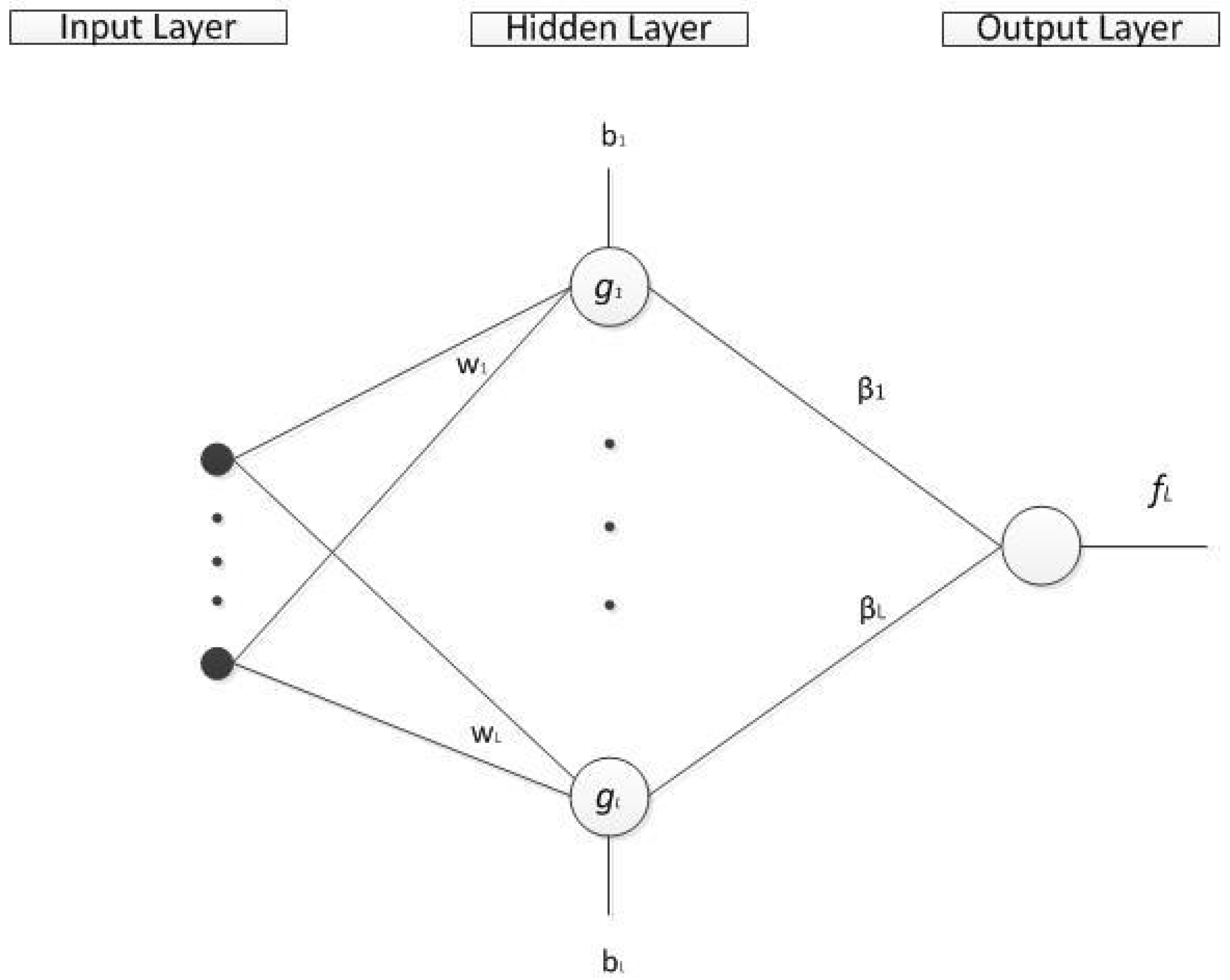
This paper focuses on the single-hidden layer feedforward network. As shown in Figure 1, it has three layers, including the input layer, the hidden layer and the output layer. Without loss of generality, this paper considers the SLFN with only one output node.
The output of SLFN with L hidden nodes is represented as follows [3]:
where is the i-th hidden node and can be one of the two following types:
- For additive nodes
- 2.
- For RBF nodes
All networks that can be generated are represented as the following functions set [3]:
where
and is a set of all possible hidden nodes. For additive nodes, we have
For the RBF case, we have
Let f be a target function that is approximated by the network with L hidden nodes. The network residual error function is defined as follows:
In practice, the function form of error is not available and the network is trained on finite data samples, which are described as , where is the d dimension input vector of the i-th training sample and is its target value. Thus, the error vector on the training samples is denoted as follows:
where is the error of the i-th training sample for the network with L hidden nodes . Furthermore, the activation vector for the L-th hidden node is
where is the output of the L-th hidden nodes for the i-th training sample .
3. Previous Work
There are several types of constructive neural networks. In this section, the networks that are proposed in [3,28] are introduced. In those methods, the network is constructed by adding a new node to the network in each step. The training process of the newly added node (L-th hidden node) is divided into two phases: the first phase is devoted to adjusting the input parameters and the second phase is devoted to adjusting the output weight. When the parameters of the new node are obtained, they are fixed and do not change during the training of the next nodes.
3.1. The Networks Introduced in [3]
For the input parameters’ adjustment in [3], several objective functions are proposed to adjust the input parameters of the newly added node in the constructive network. They are as follows [3]:
where is the objective function for the cascade correlation network, . The objective function that is used to adjust the output weight of the L-th hidden node is [3]
and is maximized if and only if [3]
which is the optimum output parameter of the new node. In [3], the authors also proved that for each of the objective functions to , the network error converges.
Theorem 1
([3]). Given span (G) is dense in and for some . If is selected so as to , then .
More detailed discussion about theorems and their proofs can be found in [3].
3.2. Cascade Correntropy Network (CCOEN) [28]
The authors in [28] proved that if the input parameters of each new node in a cascade network are assessed by using the correntropy objective function with the sigmoid kernel and its output parameter is adjusted by
then the network is a universal approximator. The following theorem investigates the approximation ability of CCOEN:
Theorem 2
([28]). Suppose is dense in . For any continuous function f and for the sequence of error similarity feedback functions , there exists a real sequence such that
holds with probability one if
It was shown that CCOEN is more robust than the networks proposed in [3] when data are contaminated by noise.
4. Proposed Method
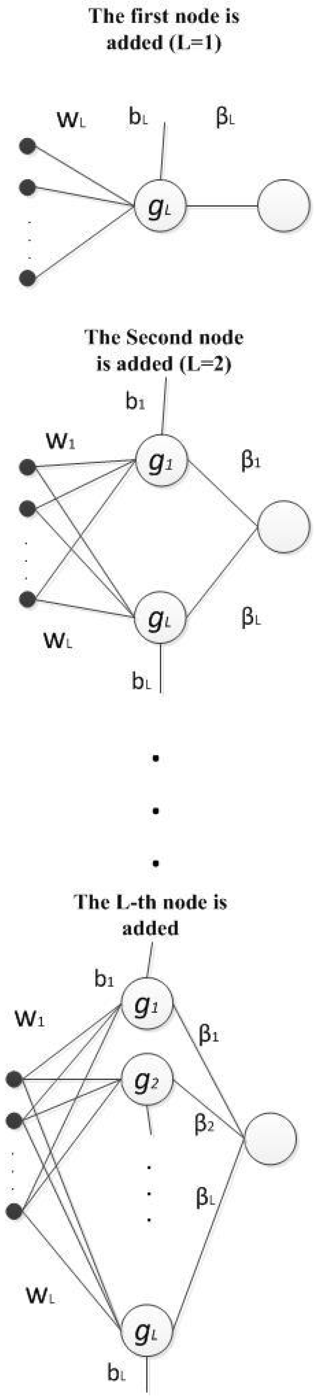
In this section, a novel constructive neural network is proposed based on the maximum correntropy criterion with the Gaussian kernel. To the best of our knowledge, it is the first time that correntropy with Gaussian kernel is employed as the objective function for training both the input and output weights of a single-hidden layer constructive network. It must be considered that the correntropy is a non-convex objective function and it is difficult to adjust the optimum solution. This section proposes a new theorem and surprisingly proves that the proposed method that is trained by using the correntropy objective function converges to the global solution. It is shown that the performance of the proposed method is excellent in the presence of non-Gaussian noise, especially impulse noise. In the proposed network, hidden nodes are added and trained one by one and the parameters of the newly added ( L-th hidden node) nodes are obtained and then fixed (see Figure 2).
This section is organized as follows: First, some preliminaries, mathematical definitions and theorems that are necessary for presenting the proposed method and proving the convergence of the method are introduced in Section 4.1. The new training strategy for the proposed method is described in Section 4.2. In Section 4.3, the convergence of the proposed method is proven when the error and activation function are continuous random variables. In practice and during the training on the dataset, the error function is not available; thus, the error vector and activation vector are used to train the new node. Regarding this fact, in Section 4.1, two optimization problems are presented to adjust the parameters of the new node based on training data samples.
4.1. Preliminaries for Presenting the Proposed Method
This section presents a new theorem for the proposed method based on special spaces, which are defined in Definitions 1 and 2.
The following lemmas, propositions and theorems are also used in the proof of the main theorem.
Lemma 1
([31]). Given is dense in for every , if and only if g is not a polynomial (almost everywhere).
Proposition 1
([32]). For , there exists a convex conjugated function ϕ, such that
Moreover, for a fixed z, the supremum is reached at .
Theorem 3
([33]). If is any sequence of random variables which are positive (take values in , increasingly converge for any , and the expectation exists for all n ), then .
Theorem 4
([33]). (Monotonicity) Let X and Y be random variables with , then , with equality if and only if almost surely.
Theorem 5
([34]). (Convergence) Every upper bounded increasing sequence converges to its supremum.
4.2. C2N2: Objective Function for Training the New Node
In this subsection, we combine the idea of constructive SLFN with the idea of correntropy and propose a new strong constructive network that is robust to impulsive noise. The proposed method employs correntropy as the objective function to adjust the input and output parameters of the network. To the best of our knowledge, it is the first time that correntropy with the Gaussian kernel has been employed for training all the parameters of a constructive SLFN. C2N2 starts with zero hidden nodes. The first hidden node is added to the network. First, the input parameters of the hidden node are calculated by employing a correntropy objective function with a Gaussian kernel. Then, they are fixed and the output parameter of the node is adjusted by the correntropy objective function with Gaussian kernel. After the parameters of the first node are obtained, they are then fixed and the next hidden node is added to the network and trained. This process is iterated until the stopping condition is satisfied.
The proposed method can be viewed as an extension of CCOEN [28] with the following differences:
- In contrast to CCOEN, which uses correntropy with a sigmoid kernel to adjust the input parameters of a cascade network, the proposed method uses correntropy with a Gaussian kernel to adjust the whole parameters of an SLFN.
- CCOEN uses correntropy to adjust the input parameters of the new node in a cascade network to provide a more robust method. However, the output parameter of the new node in a cascade network is still adjusted based on the least mean square error. In contrast, the proposed method uses correntropy with Gaussian kernel to obtain both the input and output parameters of the new node in a constructive SLFN. Therefore, the proposed method is more robust than CCOEN and other networks introduced in [3] when the dataset is contaminated by impulsive noise.
- Employing Gaussian kernel for correntropy as the objective function to adjust the network’s parameters provides a closed-form formula introduced in the next section. In other words, both the input and output parameters are adjusted by two closed-form formulas.
For the proposed network, each newly added node (L-th added node where is trained using the two phases.
In the first phase, the new node is selected from , using the following optimization problem: where
From the definition of the kernel, the most similar activation function to the residual error of L− 1 nodes network is selected from as this node is selected to maximize:
where is feature mapping. Consequently, the biggest reduction in error is obtained and the network has a more compact architecture.
In the second phase, the output parameter of the new node is adjusted whereby
These two phases are iterated and a new node is added in each iteration until the certain stopping condition is satisfied. This is discussed in Section 5.
After the parameters of the new node are tuned, the correntropy of the residual error (error of the network with L hidden nodes) is shown as
and the residual error is updated as follows:
It is important to note that this subsection only presents two optimization problems for adjusting the input and output parameters of the new node. In Section 4.4, we present a way to solve these problems.
4.3. Convergence Analysis
In this subsection, we prove that the correntropy of the newly constructed network undergoes a strictly increasing sequence and converges to its supremum. Furthermore, it is proven that the supremum equals the maximum. To prove the convergence of the correntropy of the network, the definitions, theorems and lemma that are presented in Section 4.1 are employed. To prove convergence of the proposed method, similarly to [3,28], we propose the following lemma and prove that the new node, which is obtained from the input side optimization problem, is not orthogonal to the residual error function.
Lemma 2.
Given is dense in and . There exists a real number such that is not orthogonal to , where
Employing Lemma 2 and what is mentioned in Section 4.1, the following theorem proves that the proposed method achieves its global solution.
Theorem 6.
Given an SLFN with (tangent hyperbolic) function for the additive nodes, for any continuous function f and for the sequence of hidden nodes functions, obtained based on the residual error functions, i.e., , there exists a real sequence such that
holds almost everywhere, provided that
where
The proof of Lemma 2 and Theorem 6 contain some pure mathematics contents and are placed in Appendix A.
4.4. Learning from Data Samples
In Theorem 6, we proved that the proposed network, i.e., the one hidden layer constructive neural network based on correntropy (C2N2), achieves an optimal solution. During the training process, the function form of the error is not available and the error and activation vectors are generated from the training samples. In the rest of this subsection, we propose a method to train the network from data samples.
4.4.1. Input Side Optimization
The optimization problem to adjust the input parameters is as follows:
On training data, expectation can be approximated as:
The constant term can be removed and the following problem can be solved instead :
Consider the following equality:
In this paper, the tanh function is selected as the activation function, which is bipolar and invertible. Therefore:
where ,
in which is the absolute function. The range of g (domain of is . Thus, it is necessary to rescale the error signal to be in the range. To do so, is assigned as follows:
where . Let , and therefore, the term
can be replaced by
and thus the following problem is presented to adjust the input parameters
To achieve better generalization performance, the norm of the weights needs to be kept minimized too; thus, the problem above is reformulated as
It should be considered that if , both problems from above are equivalent. Since the necessary condition for convergence is that in each step and by adding each node amount of correntropy of the error should be increased, in the experiment section, and other amounts for C are checked and the best result is selected. This guarantees convergence of the method according to Theorem 6.
The half-quadratic method is employed to adjust the input parameters. Based on Proposition 1, we have
The local solution of the above optimization problem is adjusted using the following iterative process:
i.e., the following optimization problem needs to be solved in each iterate:
Since is a constant term, it can be removed from the optimization problem. Then, the optimization problem can be multiplied by . We set . Thus, the following constraint optimization problem is obtained:
The Lagrangian is constituted as
The derivations of the Lagrangian function with respect to its variables are the following
where .
Now we consider two cases.
Case 1.
By substituting derivatives in
we obtain
Let be a diagonal matrix with ; therefore,
Case 2.
By substituting derivatives in
we obtain
Then
Thus, the input parameters are obtained by the following iterative process:
4.4.2. Output Side Optimization
When the input parameters of the new node are obtained from the previous step, the new node is named , where and the output parameter is adjusted using the following optimization problem:
The expectation can be approximated on training samples:
The constant term can be removed and the following problem can be solved instead :
Similar to the previous step, the half-quadratic method is employed to adjust the output parameter. Based on Proposition 1, we obtain
The local solution of the above optimization problem is adjusted using the following iterative process:
i.e., the following optimization problem is required to be solved in each iteration:
where is a diagonal matrix with .
The optimum output weight is adjusted by differentiating with respect to as
Finally, the output weight is adjusted by the following iterative process:
In these two phases, the parameters of the new node (L-th added node where ) are tuned and then fixed. This process is iterated for each new node until the predefined condition is satisfied. The following proposition demonstrates that for each node, the algorithm converges.
Proposition 2.
The sequences and converge.
Proof.
From Theorem 5 and Proposition 1, we have and . Thus, the non-decreasing sequence converges since the correntropy is upper bounded. □
Proposition 3.
When , the output weight that is adjusted by the correntropy criterion is equivalent to the output weight that is adjusted by the MSE-based method such as IELM.
Proof.
Suppose that , by , we have
□
The training process of the proposed method is summarized in the following Algorithm 1 (C2N2).
| Algorithm 1 C2N2 |
|
Remark 1.
The auxiliary variables and are utilized to reduce the effect of noisy data. For the samples with a high amount of error, these variables are very small; thus, these samples have slight effects on the optimization of the parameters of the network, which results in a more robust network.
5. Experimental Results
This section compares C2N2 with RBF, CCN and other constructive networks that are presented in [3]. The networks, whose hidden nodes’ input parameters are trained by the objective functions that are introduced in [3], are denoted by . In addition to the mentioned methods, the proposed method is compared to the state-of-the-art constructive networks such as the orthogonal least square cascade network (OLSCN) [4] and the one hidden layer constructive network (OHLCN) introduced in [5]. Moreover, C2N2 is also compared with state-of-the-art robust learning methods including Multi-Layer Perceptron based on MCC (MLPMCC) [17], Multi-Layer Perceptron based on Minimum Error Entropy (MLPMEE) [17] and Robust Least Square Support Vector Machine (RLS-SVM) [35] and the recent work, CCOEN [28].
The rest of this section is organized as follows. Section 5.1 describes a framework for the experiments. The presented theorem and hyperparameters and are investigated in Section 5.2. In Section 5.3, the presented method is compared to N1-N6, CCN, RBF and some state-of-the-art constructive networks including OHLCN and OLSCN. Experiments are performed on several synthetic and benchmark datasets that are contaminated with impulsive noise (one of the most popular types of non-Gaussian noise). In this part, experiments are also performed in the absence of impulsive noise. Section 5.4 compares the proposed method with state-of-the-art robust learning methods including MLPMEE, MLPMCC, RLS-SVM and CCOEN on various types of datasets.
5.1. Framework for Experiments
This part presents a framework for the experiments. The framework includes the type of activation function for C2N2 and other mentioned methods, type of kernel, kernel parameters , range of hyperparameters and dataset specification.
5.1.1. Activation Function and Kernel
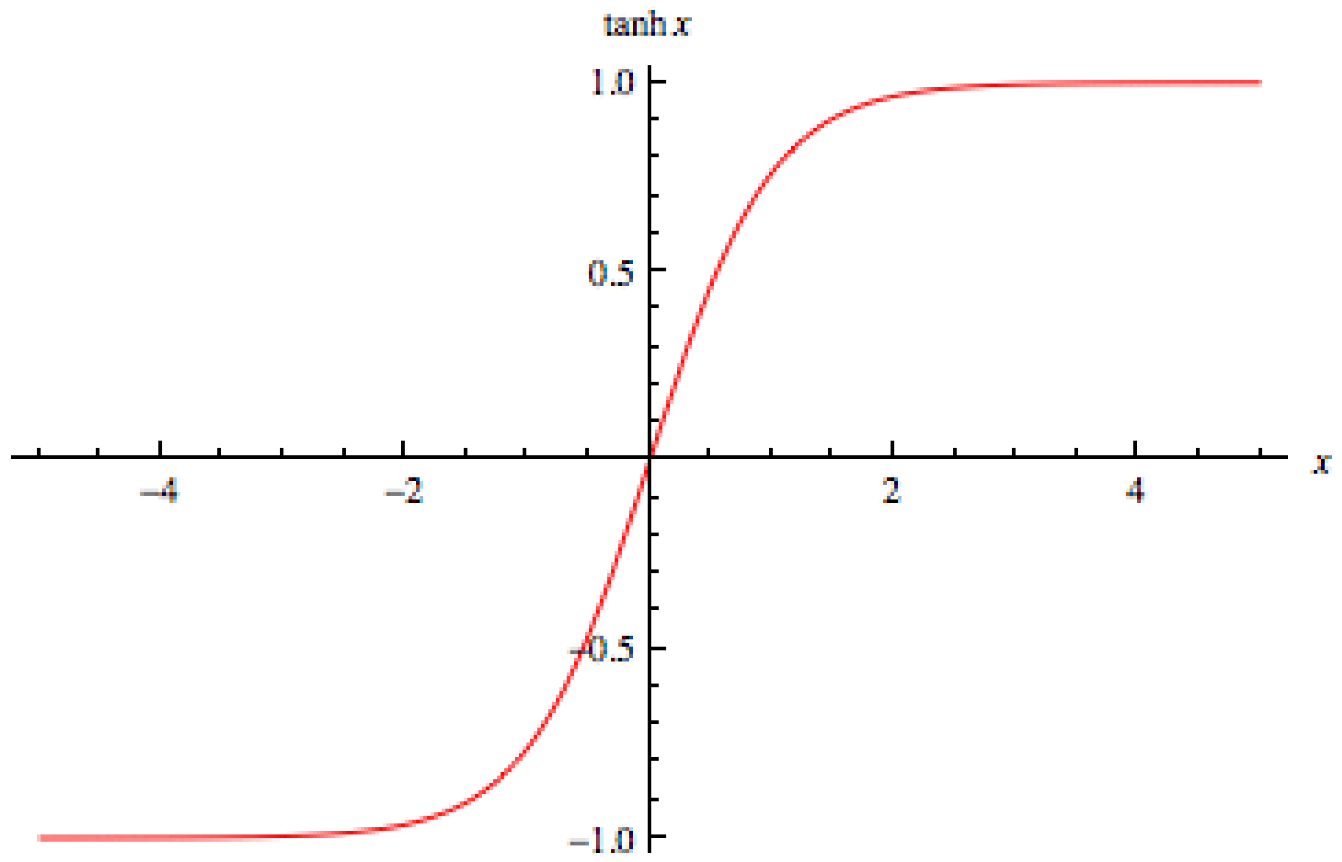
For the proposed method, the tangent hyperbolic activation function is used. It is represented as follows (see Figure 3):
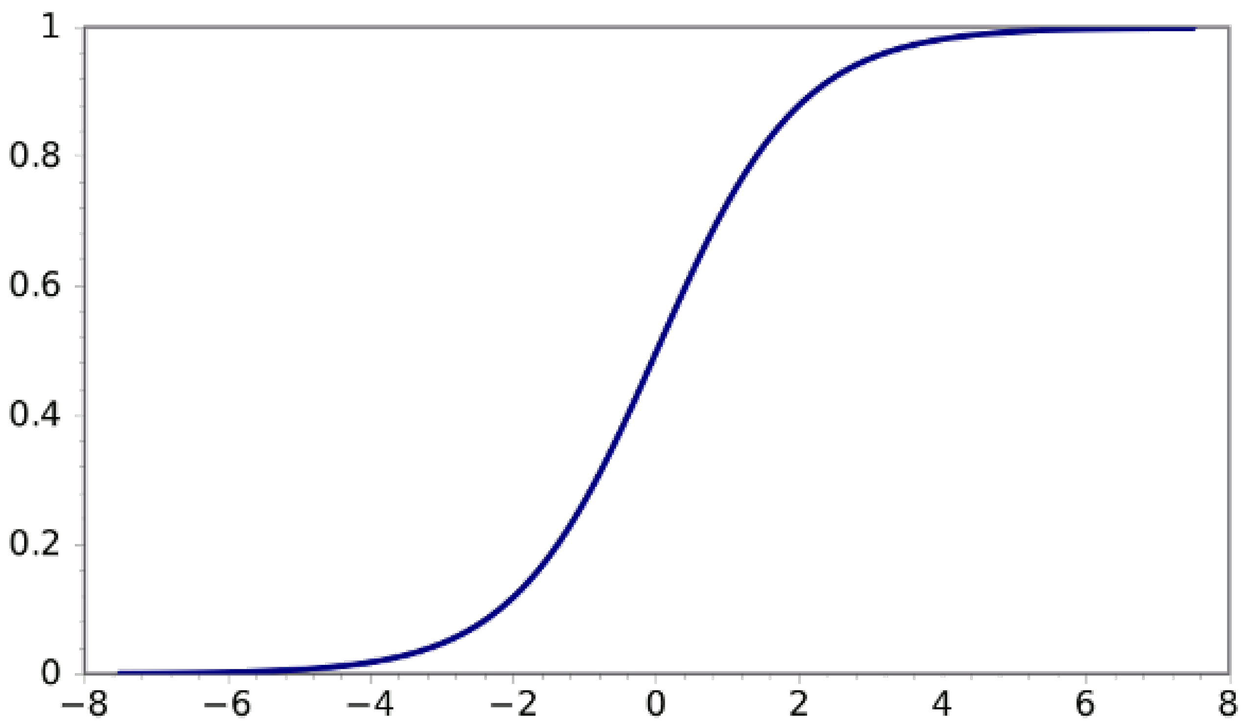
For networks , CCN, OLSCN, OHLCN, MLPMCC and MLPMEE, the sigmoid activation function is used. This function is represented and displayed as follows (see Figure 4):
For the proposed method and RLS-SVM, RBF kernel is used. It is shown as
In the experiments, the optimum kernel parameter is selected from the set
5.1.2. Hyperparameters
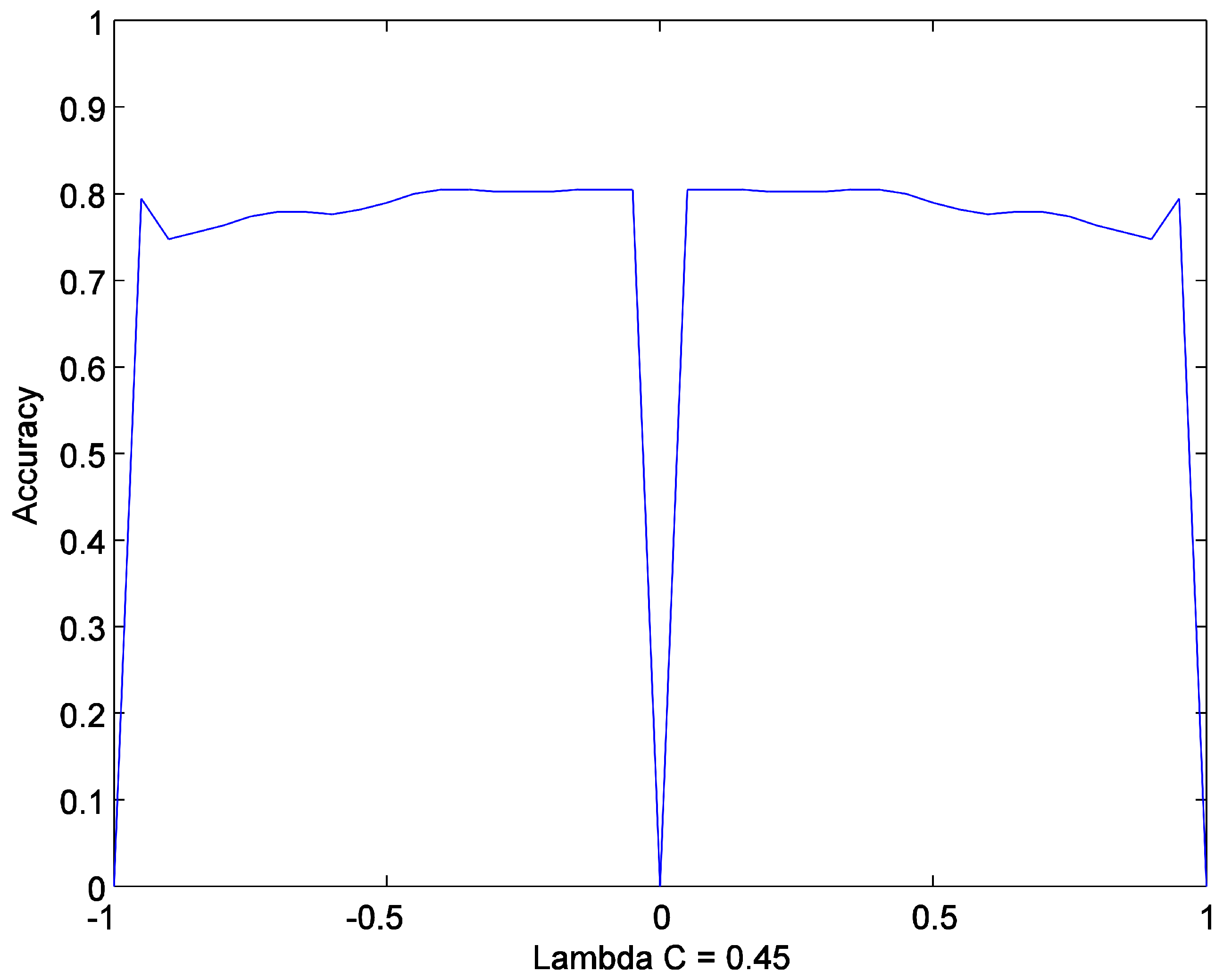
The method has three hyperparameters. These parameters help to avoid over or underfitting, which improves performance. The first parameter is a number of hidden nodes . The optimum number of hidden nodes is selected from the set . Due to the boundedness of tanh function , the error signal must be scaled to this range. Thus, should be selected from the set . Figure 5 shows that accuracy is symmetric with respect to . Thus, should be selected from the set . The possible range for is investigated in the next part.
5.1.3. Data Normalization
In this paper, the input vector of data samples is normalized into the range . For regression datasets, their targets are normalized into the range .
5.2. Convergence
This part investigates the convergence of the proposed method (Theorem 6), followed by an investigation of the hyperparameters.
5.2.1. Investigation of Theorem 6
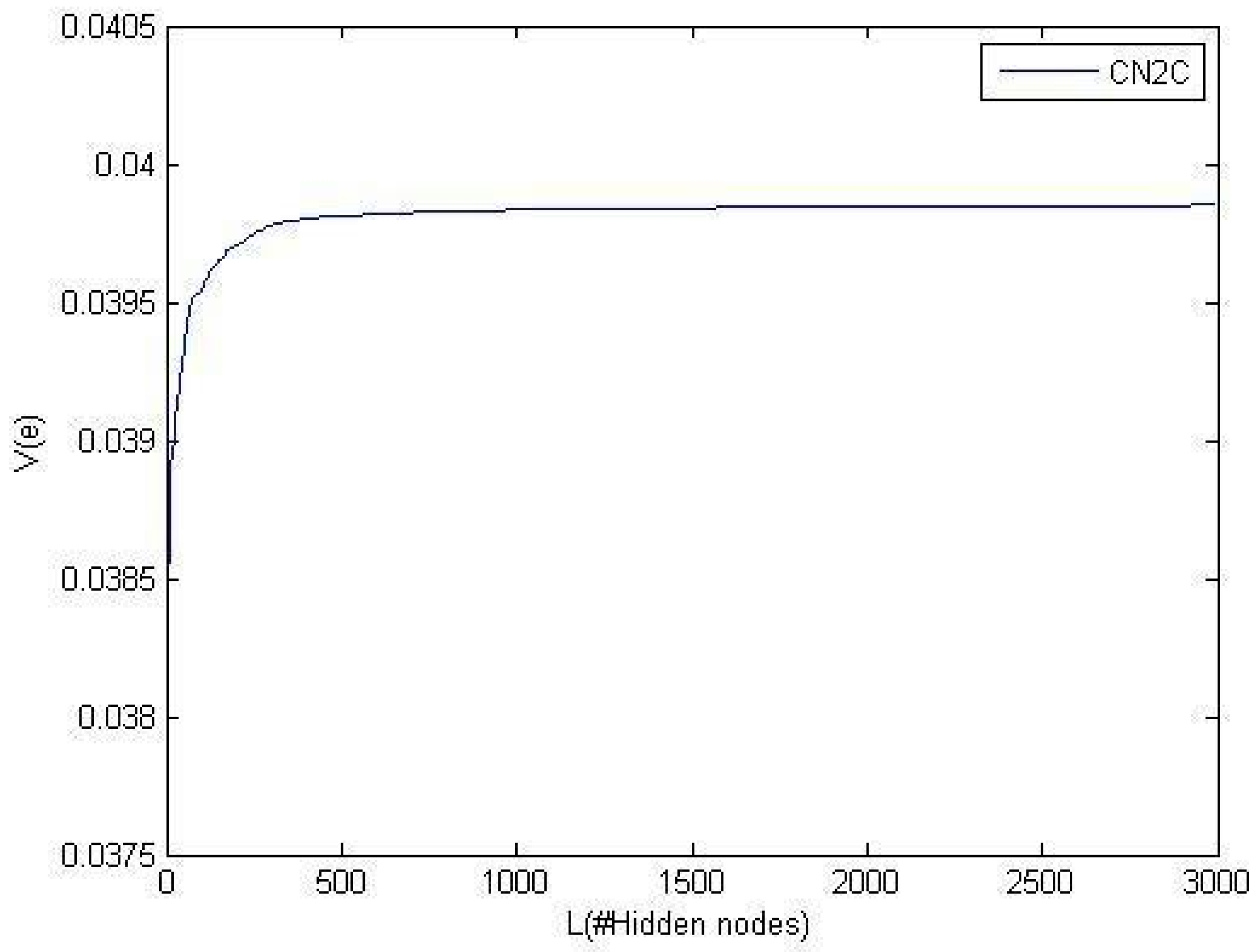
The main goal of this paper is to maximize the correntropy of the error function. Regarding the kernel definition and due to maximization of correntropy, the approximator (output of the neural network, ) has the most similarity to the target function . Theorem 6 proves that the proposed method obtains the optimal solution, i.e., the correntropy of the error function is maximized. This part investigates the convergence of the proposed method. In this experiment, the kernel parameter is set to 10; thus, the optimum value for correntropy is . Figure 6 shows the convergence of C2N2 to the optimum value in the approximation of the sinc function.
5.2.2. Hyperparameter Evaluation
To evaluate parameters and , C2N2 with only one hidden node was experimented on using the diabetes dataset. Figure 7 shows that the best amount for parameter is in the range . Thus, in the experiments, parameter is selected from the set .
5.3. Comparison
This part compares the proposed method with the networks , CCN, OHLCN, OLSCN, and RBF in the presence and absence of non-Gaussian noise. One of the worst types of non-Gaussian noise is impulsive noise.
For = 0, the accuracy is set to zero. This type of noise adversely affects the performance of MSE-based methods such as the networks , CCN, OHLCN and OLSCN. In this part and part D, we perform experiments similar to [4]. We calculated the RMSE (classification accuracy) on the testing dataset after each hidden unit was added and reported the lowest (highest) RMSE (accuracy) along with the corresponding network size. Similar to [4], experiments were carried out in 20 trials and the results (RMSE (accuracy) and number of nodes) averaged over 20 trials are listed in Table 3, Table 4, Table 5 and Table 6.
In all result tables, the best results are shown in bold and underlined. The results that are close to the best ones are in bold.
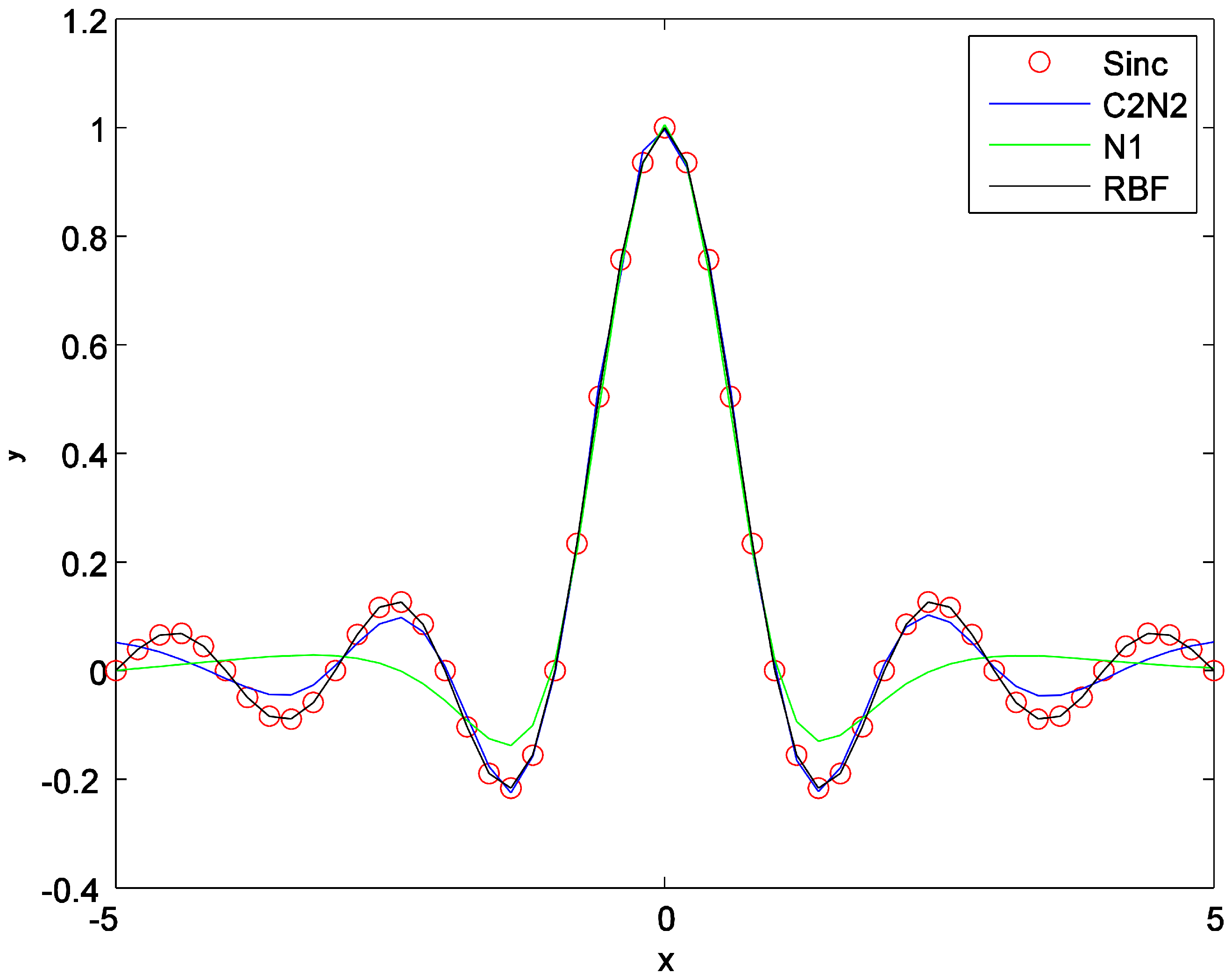
5.3.1. Synthetic Dataset (Sinc Function)
5.3.2. Other Synthetic Dataset
The following regression problems are used to evaluate the performance of the proposed method in comparison to the networks and .
where
For each of the above functions, 225 pairs are generated randomly in the interval . For each piece of training data, its target is assigned as
where is noise that is added to the target of the data samples. In this section, the index of the noise is:
For impulse noise, the outputs of five data samples are changed by extra high values using the uniform distribution.
5.4. Discussion
5.4.1. Discussion on Table 7
Table 7 compares C2N2 with the networks and . From the table, we can see that in the absence of noise, the proposed method outperforms the other methods on the datasets and . For the dataset , the best result is for the network . We added impulsive noise to the dataset and again performed experiments. From Table 7, we can see that the proposed method is more stable when data are contaminated with impulsive noise. For example, for the dataset , the RMSEs of C2N2 and to are close. However, in the presence of impulsive noise for the dataset , the RMSEs for C2N2 and to are 0.2487, 0.3676, 0.2790, and 0.3226 respectively. This means that noisy data samples have less effect on the proposed method in comparison to the other mentioned methods and the proposed method is more stable. The goal of any learning method is to increase performance. Thus, in this paper, we focus on RMSE. However, from the architecture viewpoint, the proposed method tends to have a smaller number of nodes in of the datasets.

Table 7.
Performance comparison of C2N2 and the networks and : synthetic regression dataset.
| Datasets | C2N2 | |||||||||||
|---|---|---|---|---|---|---|---|---|---|---|---|---|
|
Testing
RMSE | #N | Time (s) |
Testing
RMSE | #N | Time (s) |
Testing
RMSE | #N | Time (s) |
Testing
RMSE | #N | Time (s) | |
| 0.1358 | 0.69 | 0.1555 | 4.85 | 1.48 | 6.30 | 1.78 | 0.1536 | 7.05 | 0.81 | |||
| 6.25 | 0.91 | 0.3244 | 0.44 | 0.2460 | 0.72 | 0.2750 | 4.40 | 2.40 | ||||
| 1.09 | 5.90 | 1.91 | 4.55 | 1.57 | 5.45 | 2.18 | ||||||
| 3.98 | 0.3676 | 5.25 | 1.08 | 0.2790 | 0.89 | 0.3226 | 5.65 | 1.16 | ||||
| 1.05 | 0.0940 | 6.80 | 0.12 | 0.0943 | 1.34 | 0.0935 | 6.40 | 0.34 | ||||
| 4.15 | 1.12 | 0.2949 | 4.15 | 0.64 | 0.2309 | 0.51 | 0.2555 | 4.35 | 0.57 | |||
| 1.81 | 4.55 | 1.34 | 8.10 | 2.02 | 0.1963 | 4.70 | 0.87 | |||||
| 7.70 | 3.01 | 0.2928 | 1.54 | 0.2569 | 4.20 | 0.98 | 0.2961 | 4.85 | 0.45 | |||
5.4.2. Why C2N2 Denies Impulse Noises?
Regarding optimization problems, for noisy (impulsive noise) data, auxiliary variables are low. Thus, such data have a small role in optimization problems; parameters of the new node are obtained based on noise-free data (Remark 1). Table 8 shows the auxiliary variables for several noisy and noise-free data samples.
5.4.3. Benchmark Dataset
In this part, several regression and classification datasets are contaminated with impulse noise. At this time, as in [38], we produce impulsive noise by generating random real numbers from the following distribution function, and then we add them to data samples:
where is a Gaussian distribution function with the mean and variance . For the regression dataset, we add noise to its target. For the classification dataset, we add noise to its input feature vector. Experiments on these datasets confirm the robustness of the proposed method in comparison with , CCN and RBF, OLSCN and OHLCN.
5.4.4. Discussion on Table 3
Table 3 compares C2N2 with the networks , CCN and RBF on the Autoprice, Baloon and Pyrim datasets in the presence and absence of impulsive noise. It shows that C2N2 is more stable than the networks N4 to N6, CCN and RBF in the presence of non-Gaussian noise. For example, for the Autoprice dataset, RMSEs for C2N2, N4-N6, CCN and RBF are and , respectively. After adding noise, RMSEs are and respectively. These results confirm that the proposed method is robust to impulsive noise in comparison to the mentioned methods.
5.4.5. Discussion on Table 4
This table compares C2N2 with the networks , CCN and RBF on the Ionosphere, Colon, Leukemia and Dimdata datasets in the presence of impulsive noise. It shows that C2N2 outperforms the other mentioned methods on the Ionosphere, Colon and Leukemia datasets. For the dataset Dimdata, RBF outperforms the proposed method. However, the result is obtained with 1000 nodes for and with an average of nodes for C2N2.
5.4.6. Discussion on Table 5 and Table 6
These tables compare C2N2 with state-of-the-art constructive networks on the regression and classification datasets. They show that the best results are for C2N2. For the Housing dataset, RMSEs for C2N2, OLSCN and OHLCN are and , respectively. In the presence of impulsive noise, RMSEs are and . Thus, the proposed method has the best stability among the other mentioned state-of-the-art constructive networks when data samples are contaminated with impulsive noise. From the architecture viewpoint, OLSCN has the most compact architecture. However, it has the worst training time. Table 6 shows that C2N2 outperforms OLSCN and OHLCN in the presence of impulsive noise in the classification dataset.
5.4.7. Computational Complexity
Let L be the maximum number of hidden units to be added to the network. For each newly added node, its input parameter is adjusted as specified in Section 4.4.1. The order of adjusting the inverse of the matrix is . Thus, , where k is the constant term (number of iterations). Thus, we have
5.5. Comparison
This part compares C2N2 with state-of-the-art robust learning methods on several benchmark datasets. These methods are Robust Least Square SVM (RLS-SVM), MLPMEE and MLPMCC. As mentioned in Section 5.4, and similar to [4], in this part, experiments are performed in 20 trials and average results of RMSE (accuracy for classification) and the number of hidden nodes(#N) are reported in Table 9.
5.5.1. Discussion on Table 9
From the table, we can see that for Pyrim, Prim (noise) and baskball (noise), C2N2 absolutely outperforms the other robust methods in terms of RMSE. For Bodyfat and Bodyfat (noise), C2N2 slightly outperforms other methods in terms of RMSE. Thus, to compare them, we need to check the number of nodes and training times. For both datasets, C2N2 has a fewer number of nodes. In the presence of noise, C2N2 has a better training time in comparison to RLS-LSVM.
Thus, the proposed method outperforms the other methods for these two datasets. Among these six datasets, RLS-SVM only outperforms C2N2 in one dataset, i.e., Baskball; however, it has a worse training time and more nodes. It can be seen that among the robust methods, the proposed method has the most compact architecture.
5.5.2. Discussion on Table 10
This table compares the recent work, CCOEN, with the proposed method on three datasets in the presence and absence of noise. According to the table, the proposed method outperforms CCOEN in all cases except the Cloud dataset in the presence of noise where CCOEN has a slightly better performance with more hidden nodes. From the architecture viewpoint, the proposed method has a fewer number of nodes in comparison to CCOEN in most cases. Therefore, correntropy with the Gaussian kernel provides better results in comparison to the sigmoid kernel.
Table 10.
Performance comparison of C2N2 and the recent work. CCOEN: benchmark regression dataset.
| Dataset | C2N2 | CCOEN | ||
|---|---|---|---|---|
| Testing RMSE | #Nodes | Testing RMSE | #Nodes | |
| Abalone | 0.090 | 8.8 | ||
| Abalone (Noise) | 7.8 | |||
| Cleveland | 0.791 | 6.1 | ||
| Cleveland (Noise) | 0.821 | 8.5 | ||
| Cloud | 0.293 | 4.7 | ||
| Cloud (noise) | 0.302 | 5.6 | ||
6. Conclusions
In this paper, a new constructive feedforward network is presented that is robust to non-Gaussian noises. Most of the other existing constructive networks are trained based on the mean square error (MSE) objective function and consequently act weak in the presence of non-Gaussian noises, especially impulsive noise. Correntropy is a local similarity measure of two random variables and is successfully used as the objective function for the training of adaptive systems such as adaptive filters. In this paper, this objective function with a Gaussian kernel is utilized to adjust the input and output parameters of the newly added node in a constructive network. It is proved that the new node obtained from the input side optimization is not orthogonal to the residual error of the network. Regarding this fact, correntropy of the residual error converges to its optimum when the error and the activation function are continuous random variables in space where the triple is considered as a probability space. During the training on datasets, the function form of error is not available; thus, we provide a method to adjust the input and output parameters of the new node from training data samples. The auxiliary variables that appear in input and output side optimization problems decrease the effect of the non-Gaussian noises. For example, for impulsive noise, these variables are close to zero; thus, these data samples have little role in optimizing the parameters of the network. For the MSE-based constructive networks, the data samples that are contaminated by impulsive noises have a great role in optimizing the parameters of the network, and consequently, the network is not robust. The experiments are performed on some synthetic and benchmark datasets. For the synthetic datasets, the experiments are performed in the presence and absence of impulsive noises. We saw that for the datasets that are contaminated by impulsive noises, the proposed method has significantly better performance than the state-of-the-art MSE-based constructive network. For the other synthetic and benchmark datasets, in most cases, the proposed method has satisfactory performance in comparison to the MSE-based constructive network and radial basis function (RBF). Furthermore, C2N2 was compared with state-of-the-art robust learning methods such as MLPMEE, MLPMCC and the robust version of the Least Square Support Vector Machine and CCOEN. The performances are obtained with compact architectures due to the input parameters being optimized. We also see that correntropy with Gaussian kernel provides better results in comparison to the correntropy with sigmoid kernel.
The use of the correntropy-based function introduced in this research may also benefit networks with other architectures toward enhancing the generalization performance and robustness level. In the context of further research, the validity of similar results can be verified for various classes of neural networks. In addition, since impulsive noise is one of the worst cases of non-Gaussian noise, it can be expected that a different non-Gaussian noise will yield a result between clean data and data with impulsive noise. This should be verified in further experiments.
It is also necessary to point out here other novel modern avenues and similar research directions. For example, ref. [39] delves into modal regression, presenting a statistical learning perspective that could enrich the discussion on learning algorithms and their efficiency in different noise conditions. In particular, it points out that correntropy-based regression can be interpreted from a modal regression viewpoint when the tuning parameter goes to zero. At the same time, [40] depicts a big picture of correntropy-based regression by showing that with different choices of the tuning parameter, correntropy-based regression learns a location function.
Correntropy not only has inferential properties that could be used for neural network analysis, but another approach could be, for example, cross-sample entropy-based techniques. One such direction was shown to be effective in [41] with reported results of simulation on exchange market datasets.
Finally, it is also worth mentioning that the choice of the algorithm applied for optimizing the objective functions can influence the results. The usage of non-smooth methodology focusing on bundle-based algorithms [42] as a possible efficient tool in machine learning and neural network analysis can also be tested.
Author Contributions
All authors contributed to the paper. The experimental part was mainly done by the first author, M.N. Conceptualization was done by M.R. and H.S.Y. Verification and final editing of the manuscript was done by Y.N., A.M. and M.M.M. who played a role of a research director. All authors have read and agreed to the published version of the manuscript.
Funding
This research received no external funding.
Data Availability Statement
Data and codes can be requested from the first author.
Acknowledgments
The authors would like to express their thanks to the GA. Hodtani and Ehsan Shams Davodly for their constructive remarks and suggestions.
Conflicts of Interest
The authors declare no conflicts of interest.
Abbreviations
The following abbreviations are used in this manuscript:
| C2N2 | Correntropy-based constructive neural network |
| MCC | Maximum correntropy criterion |
| MSE | Mean square error |
| MEE | Minimum Error Entropy |
| EMSE | Excess mean square error |
| OLS | Orthogonal least square |
| CCOEN | Cascade correntropy network |
| MLPMEE | Multi-Layer Perceptron based on Minimum Error Entropy |
| MLPMCC | Multi-Layer Perceptron based on correntropy |
| RLS-SVM | Robust Least Square Support Vector Machine |
| FFN | Feedforward network |
| RBF | Radial basis function |
| ITL | Information theoretic learning |
| CGN | Cascade correlation network |
| OHLCN | One hidden layer constructive adaptive neural network |
Appendix A
Appendix A.1. Proof of Lemma 1
Proof.
Similar to [28], let where
Thus,
Let , we have,
We need to prove that exists such that
Suppose that the inequality above does not hold.
Two possible conditions may happen:
1.1. If , we have
Again, there are two possible conditions: First, . Then
.
.
Let . From the assumption and the above inequality, we have .
This is contradicted by the fact that is dense in . Second: .
.
.
Let .
From the assumption above, we have .
This is contradicted by the fact that is dense in .
- 2.
2.1. If , we have
Again, there are two possible conditions: First: . Then
,
.
Let .
.
From the assumption, we have .
This is contradicted by the fact that is dense in . Second:
.
.
Let .
From the assumption above, we have, , and this is contradicted by the fact that is dense in . Based on the above arguments, a real number exists such that the following inequality holds:
Thus, from Theorem 4, we have
Thus, there exists a real number such that
This means that and this completes the proof. □
Appendix A.2. Proof of Theorem 6
Proof.
Inspired by [3], the proof of this theorem is divided into two parts: First, we prove that the correntropy of the network strictly increases after adding each hidden node, and then we prove that the supremum of the correntropy of the network is .
Step 1: The correntropies of an SLFN with and L hidden nodes are:
respectively.
In the following, it is proved that exists such that
Let
then we have
where
Thus,
We need to prove that and exist such that
Suppose that there are no and such that
and
Then the following inequality holds,
.
and
and .
Let
Thus, . This is contradictory to being dense in ; thus, we have
.
Based on Theorem 4, the following inequality holds with probability one:
, i.e.,
almost surely.
Based on the above argument, with probability one, we have:
Based on Theorem 5, since the correntropy is strictly increasing, with probability one it converges to its supremum.
Step 2: We know that
and according to Proposition 1, we have
There is
Therefore, the optimum is
In the previous step, we showed that correntropy converges; the norm of error converges and converges to a constant term. In the case of constant , similar to [3], the error sequence constitutes a Cauchy sequence and because the mentioned probability space is complete, . Therefore,
Thus, similar to [3], we have
As we know, , and we have
and
Based on Theorem 3 and , we have . Based on step 1 and step 2, we have almost surely.
This completes the proof. □
References
- Erdogmus, D.; Principe, J.C. An error-entropy minimization algorithm for supervised training of nonlinear adaptive systems. Signal Process. IEEE Trans. 2002, 50, 1780–1786. [Google Scholar] [CrossRef]
- Fahlman, S.E.; Lebiere, C. The cascade-correlation learning architecture. In Proceedings of the Advances in Neural Information Processing Systems 2, NIPS Conference, Denver, CO, USA, 27–30 November 1989; pp. 524–532. [Google Scholar]
- Kwok, T.-Y.; Yeung, D.-Y. Objective functions for training new hidden units in constructive neural networks. Neural Netw. IEEE Trans. 1997, 8, 1131–1148. [Google Scholar] [CrossRef] [PubMed]
- Huang, G.; Song, S.; Wu, C. Orthogonal least squares algorithm for training cascade neural networks. Circuits Syst. Regul. Pap. IEEE Trans. 2012, 59, 2629–2637. [Google Scholar] [CrossRef]
- Ma, L.; Khorasani, K. New training strategies for constructive neural networks with application to regression problems. Neural Netw. 2004, 17, 589–609. [Google Scholar] [CrossRef] [PubMed]
- Ma, L.; Khorasani, K. Constructive feedforward neural networks using Hermite polynomial activation functions. Neural Netw. IEEE Trans. 2005, 16, 821–833. [Google Scholar] [CrossRef] [PubMed]
- Reed, R. Pruning algorithms-a survey. Neural Netw. IEEE Trans. 1993, 4, 740–747. [Google Scholar] [CrossRef] [PubMed]
- Castellano, G.; Fanelli, A.M.; Pelillo, M. An iterative pruning algorithm for feedforward neural networks. Neural Netw. IEEE Trans. 1997, 8, 519–531. [Google Scholar] [CrossRef] [PubMed]
- Engelbrecht, A.P. A new pruning heuristic based on variance analysis of sensitivity information. Neural Netw. IEEE Trans. 2001, 12, 1386–1399. [Google Scholar] [CrossRef]
- Zeng, X.; Yeung, D.S. Hidden neuron pruning of multilayer perceptrons using a quantified sensitivity measure. Neurocomputing 2006, 69, 825–837. [Google Scholar] [CrossRef]
- Sakar, A.; Mammone, R.J. Growing and pruning neural tree networks. Comput. IEEE Trans. 1993, 42, 291–299. [Google Scholar] [CrossRef]
- Huang, G.-B.; Saratchandran, P.; Sundararajan, N. A generalized growing and pruning RBF (GGAPRBF) neural network for function approximation. Neural Netw. IEEE Trans. 2005, 16, 57–67. [Google Scholar] [CrossRef]
- Huang, G.-B.; Saratchandran, P.; Sundararajan, N. An efficient sequential learning algorithm for growing and pruning RBF (GAP-RBF) networks. Syst. Man. Cybern. Part Cybern. IEEE Trans. 2004, 34, 2284–2292. [Google Scholar] [CrossRef] [PubMed]
- Wu, X.; Rozycki, P.; Wilamowski, B.M. A Hybrid Constructive Algorithm for Single-Layer Feedforward Networks Learning. IEEE Trans. Neural Netw. Learn. Syst. 2014, 26, 1659–1668. [Google Scholar] [CrossRef] [PubMed]
- Santamaría, I.; Pokharel, P.P.; Principe, J.C. Generalized correlation function: Definition, properties, and application to blind equalization. Signal Process. IEEE Trans. 2006, 54, 2187–2197. [Google Scholar] [CrossRef]
- Liu, W.; Pokharel, P.P.; Príncipe, J.C. Correntropy: Properties and applications in non-Gaussian signal processing. Signal Process. IEEE Trans. 2007, 55, 5286–5298. [Google Scholar] [CrossRef]
- Bessa, R.J.; Miranda, V.; Gama, J. Entropy and correntropy against minimum square error in offline and online three-day ahead wind power forecasting. Power Syst. IEEE Trans. 2009, 24, 1657–1666. [Google Scholar] [CrossRef]
- Singh, A.; Principe, J.C. Using correntropy as a cost function in linear adaptive filters. In Proceedings of the 2009 International Joint Conference on Neural Networks, Atlanta, GA, USA, 14–19 June 2009; pp. 2950–2955. [Google Scholar]
- Shi, L.; Lin, Y. Convex Combination of Adaptive Filters under the Maximum Correntropy Criterion in Impulsive Interference. Signal Process. Lett. IEEE 2014, 21, 1385–1388. [Google Scholar] [CrossRef]
- Zhao, S.; Chen, B.; Principe, J.C. Kernel adaptive filtering with maximum correntropy criterion. In Proceedings of the 2011 International Joint Conference on Neural Networks, San Jose, CA, USA, 31 July–5 August 2011; pp. 2012–2017. [Google Scholar]
- Wu, Z.; Peng, S.; Chen, B.; Zhao, H. Robust Hammerstein Adaptive Filtering under Maximum Correntropy Criterion. Entropy 2015, 17, 7149–7166. [Google Scholar] [CrossRef]
- Chen, B.; Wang, J.; Zhao, H.; Zheng, N.; Principe, J.C. Convergence of a fixed-point algorithm under Maximum Correntropy Criterion. Signal Process. Lett. IEEE 2015, 22, 1723–1727. [Google Scholar] [CrossRef]
- Chen, B.; Xing, L.; Liang, J.; Zheng, N.; Principe, J.C. Steady-state mean-square error analysis for adaptive filtering under the maximum correntropy criterion. Signal Process. Lett. IEEE 2014, 21, 880–884. [Google Scholar]
- Chen, L.; Qu, H.; Zhao, J.; Chen, B.; Principe, J.C. Efficient and robust deep learning with Correntropyinduced loss function. Neural Comput. Appl. 2015, 27, 1019–1031. [Google Scholar] [CrossRef]
- Singh, A.; Principe, J.C. A loss function for classification based on a robust similarity metric. In Proceedings of the 2010 International Joint Conference on Neural Networks (IJCNN), Barcelona, Spain, 18–23 July 2010; pp. 1–6. [Google Scholar]
- Feng, Y.; Huang, X.; Shi, L.; Yang, Y.; Suykens, J.A. Learning with the maximum correntropy criterion induced losses for regression. J. Mach. Learn. Res. 2015, 16, 993–1034. [Google Scholar]
- Chen, B.; Príncipe, J.C. Maximum correntropy estimation is a smoothed MAP estimation. Signal Process. Lett. IEEE 2012, 19, 491–494. [Google Scholar] [CrossRef]
- Nayyeri, M.; Yazdi, H.S.; Maskooki, A.; Rouhani, M. Universal Approximation by Using the Correntropy Objective Function. IEEE Trans. Neural Netw. Learn. Syst. 2018, 29, 4515–4521. [Google Scholar] [CrossRef]
- Athreya, K.B.; Lahiri, S.N. Measure Theory and Probability Theory; Springer Science & Business Media: New York, NY, USA, 2006. [Google Scholar]
- Fournier, N.; Guillin, A. On the rate of convergence in Wasserstein distance of the empirical measure. Probab. Theory Relat. Fields 2015, 162, 707–738. [Google Scholar] [CrossRef]
- Leshno, M.; Lin, V.Y.; Pinkus, A.; Schocken, S. Multilayer feedforward networks with a nonpolynomial activation function can approximate any function. Neural Netw. 1993, 6, 861–867. [Google Scholar] [CrossRef]
- Yuan, X.-T.; Hu, B.-G. Robust feature extraction via information theoretic learning. In Proceedings of the 26th Annual International Conference on Machine Learning, Montreal, QC, Canada, 14–18 June 2009; pp. 1193–1200. [Google Scholar]
- Klenke, A. Probability Theory: A Comprehensive Course; Springer Science & Business Media: New York, NY, USA, 2013. [Google Scholar]
- Rudin, W. Principles of Mathematical Analysis; McGraw-Hill: New York, NY, USA, 1964; Volume 3. [Google Scholar]
- Yang, X.; Tan, L.; He, L. A robust least squares support vector machine for regression and classification with noise. Neurocomputing 2014, 140, 41–52. [Google Scholar] [CrossRef]
- Newman, D.; Hettich, S.; Blake, C.; Merz, C.; Aha, D. UCI Repository of Machine Learning Databases; Department of Information and Computer Science, University of California: Irvine, CA, USA, 1998; Available online: https://archive.ics.uci.edu/ (accessed on 29 November 2023).
- Meyer, M.; Vlachos, P. Statlib. 1989. Available online: https://lib.stat.cmu.edu/datasets/ (accessed on 29 November 2023).
- Pokharel, P.P.; Liu, W.; Principe, J.C. A low complexity robust detector in impulsive noise. Signal Process. 2009, 89, 1902–1909. [Google Scholar] [CrossRef]
- Feng, Y.; Fan, J.; Suykens, J.A. A Statistical Learning Approach to Modal Regression. J. Mach. Learn. Res. 2020, 21, 1–35. [Google Scholar]
- Feng, Y. New Insights into Learning with Correntropy-Based Regression. Neural Comput. 2021, 33, 157–173. [Google Scholar] [CrossRef]
- Ramirez-Parietti, I.; Contreras-Reyes, J.E.; Idrovo-Aguirre, B.J. Cross-sample entropy estimation for time series analysis: A nonparametric approach. Nonlinear Dyn. 2021, 105, 2485–2508. [Google Scholar] [CrossRef]
- Bagirov, A.; Karmitsa, N.; Mäkelä, M.M. Introduction to Nonsmooth Optimization: Theory, Practice and Software; Springer International Publishing: Cham, Switzerland; Heidelberg, Germany, 2014; Volume 12. [Google Scholar]
Figure 1.
SLFN with additive nodes.

Figure 2.
Constructive network in which the last added node is referred to by L.

Figure 3.
Tangent hyperbolic function.

Figure 4.
Sigmoid function.

Figure 5.
Effect of on accuracy. Parameter is set to . The experiment is performed on the diabetes dataset with the network with only one hidden node.
Figure 5.
Effect of on accuracy. Parameter is set to . The experiment is performed on the diabetes dataset with the network with only one hidden node.

Figure 6.
Convergence of the proposed method in the approximation of Sinc function when . It converges to .
Figure 6.
Convergence of the proposed method in the approximation of Sinc function when . It converges to .

Figure 7.
Effect of hyperparameters on accuracy.

Figure 8.
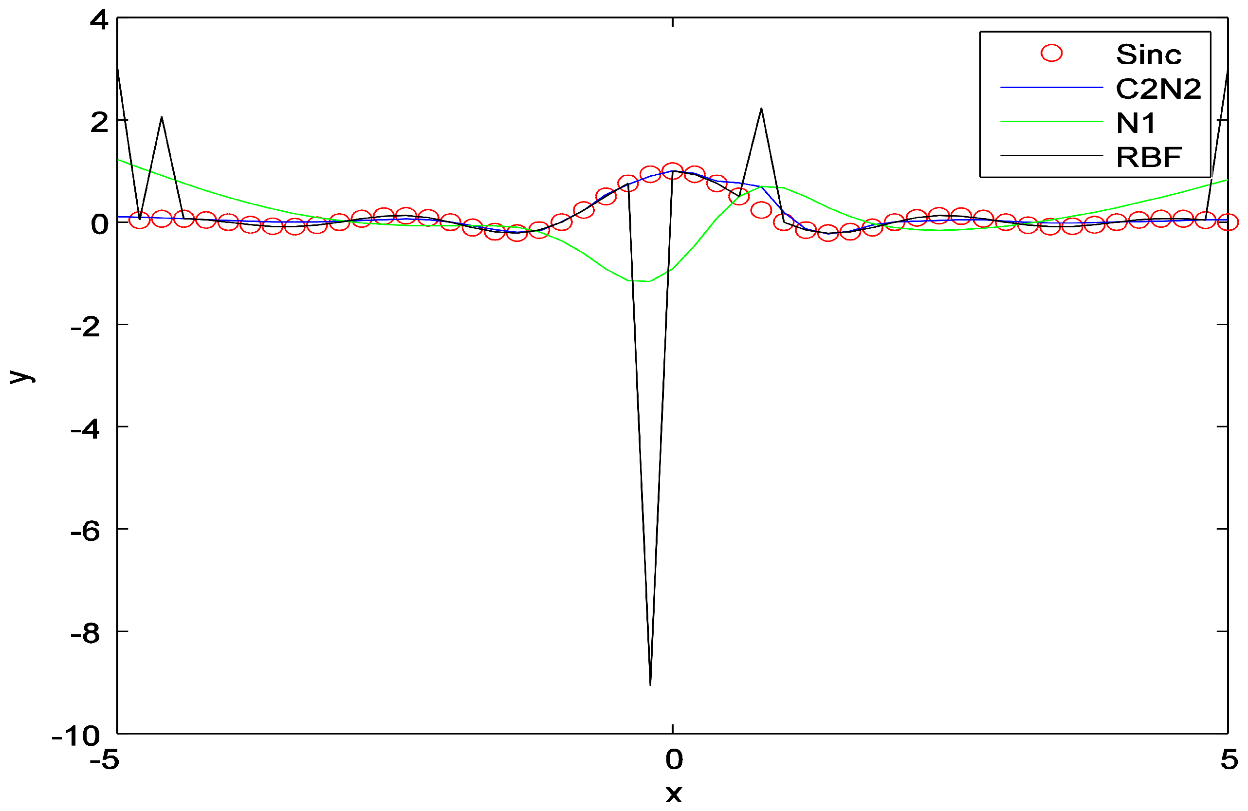
Comparison of C2N2 with RBF and the network . The experiment is performed on the approximation of the Sinc function.
Figure 8.
Comparison of C2N2 with RBF and the network . The experiment is performed on the approximation of the Sinc function.

Figure 9.
Comparison of C2N2 with RBF and the network . The experiment is performed on the approximation of the Sinc function and in the presence of impulsive noise.
Figure 9.
Comparison of C2N2 with RBF and the network . The experiment is performed on the approximation of the Sinc function and in the presence of impulsive noise.

Table 1.
Specification of the regression problem.
| Datasets | #Train | #Test | #Features |
|---|---|---|---|
| Baskball | 64 | 32 | 4 |
| Strike | 416 | 209 | 6 |
| Bodyfat | 168 | 84 | 14 |
| Quake | 1452 | 726 | 3 |
| Autoprice | 106 | 53 | 9 |
| Baloon | 1334 | 667 | 2 |
| Pyrim | 49 | 25 | 27 |
| Housing | 337 | 169 | 13 |
| Abalone | 836 | 3341 | 8 |
| Cleveland | 149 | 148 | 13 |
| Cloud | 54 | 54 | 7 |
Table 2.
Specification of the classification problem.
| Dataset | #Train | #Test | #Features |
|---|---|---|---|
| Ionosphere | 175 | 176 | 34 |
| Australian Credit | 460 | 230 | 6 |
| Diabetes | 512 | 256 | 8 |
| Colon | 32 | 30 | 2000 |
| Liver | 230 | 115 | 6 |
| Leukemia | 36 | 36 | 7129 |
| Dimdata | 1000 | 3192 | 14 |
Table 3.
Performance comparison of C2N2 and the networks , CCN and RBF: benchmark regression dataset.
Table 3.
Performance comparison of C2N2 and the networks , CCN and RBF: benchmark regression dataset.
| Datasets | C2N2 | CCN | RBF | |||||||||||||||
|---|---|---|---|---|---|---|---|---|---|---|---|---|---|---|---|---|---|---|
|
Testing
RMSE | #N |
Time
(s) |
Testing
RMSE |
Time
(s) |
Testing
RMSE |
Time
(s) |
Testing
RMSE |
Time
(s) |
Testing
RMSE |
Time
(s) |
Testing
RMSE |
Time
(s) | ||||||
| Autoprice | 4.8 | 0.54 | 0.2996 | 2 | 1.49 | 9.2 | 3.99 | 0.3681 | 5 | 6.99 | 0.2758 | 1.67 | 0.2725 | 79 | 0.008 | |||
| Autoprice (Noise) | 6.7 | 0.70 | 0.5521 | 1.07 | 0.3610 | 2.60 | 0.43 | 0.4295 | 3.77 | 1.41 | 0.4768 | 1.89 | 0.9082 | 79 | 0.009 | |||
| Baloon | 0.1065 | 5.9 | 10.73 | 0.1163 | 5.75 | 5.21 | 0.1066 | 10 | 4.96 | 0.1257 | 8.3 | 9.97 | 0.1317 | 2.09 | 150 | 0.086 | ||
| Baloon (Noise) | 5.1 | 3.25 | 0.1166 | 1.32 | 0.1252 | 8.9 | 4.66 | 0.1281 | 5 | 3.31 | 0.1358 | 2.9 | 2.12 | 1501 | 0.1351 | |||
| Pyrim | 6.7 | 0.23 | 0.0843 | 0.27 | 0.2062 | 0.07 | 0.1696 | 0.17 | 0.1694 | 0.17 | 0.0842 | 37 | 0.0090 | |||||
| Pyrim (noise) | 4.9 | 0.16 | 0.6666 | 0.32 | 0.4150 | 0.036 | 0.6203 | 0.62 | 0.5712 | 0.62 | 1.5034 | 37 | 0.0043 | |||||
Table 4.
Performance comparison of RBF, , CCN and C2N2: classification datasets.
| Datasets | RBF | CCN | C2N2 | |||||||||||||||
|---|---|---|---|---|---|---|---|---|---|---|---|---|---|---|---|---|---|---|
|
Testing
Rate (%) |
Time
(s) |
Testing
Rate (%) |
Time
(s) |
Testing
Rate (%) |
Time
(s) |
Testing
Rate (%) |
Time
(s) |
Testing
Rate (%) |
Time
(s) |
Testing
Rate (%) |
Time
(s) | |||||||
| Ionospher | 70.97 | 0.12 | 65.45 | 0.11 | 78.98 | 2.40 | 0.25 | 82.61 | 175 | 0.14 | 78.04 | 0.21 | 1.30 | 0.22 | ||||
| Colon | 62.00 | 0.02 | 63.00 | 0.03 | 62.33 | 0.38 | 90.50 | 32 | 0.12 | 64.04 | 0.29 | 0.15 | ||||||
| Leukemia | 64.44 | 0.03 | 64.44 | 0.05 | 72.44 | 0.04 | 88.61 | 36 | 0.22 | 83.71 | 0.31 | 94.72 | 1 | 0.20 | ||||
| Dimdata | 89.74 | 7.05 | 15.31 | 88.44 | 6.60 | 9.39 | 88.77 | 4.30 | 7.34 | 1000 | 4.36 | 88.37 | 8.98 | 93.73 | 3.50 | 8.29 | ||
Table 5.
Performance comparison of C2N2 and the state-of-the-art constructive networks OLSCN and OHLCN: benchmark regression dataset.
Table 5.
Performance comparison of C2N2 and the state-of-the-art constructive networks OLSCN and OHLCN: benchmark regression dataset.
| Dataset | C2N2 | OLSCN | OHLCN | ||||||
|---|---|---|---|---|---|---|---|---|---|
|
Testing
RMSE | #Nodes |
Time
(s) |
Testing
RMSE | #Nodes |
Time
(s) |
Testing
RMSE | #Nodes |
Time
(s) | |
| Housing | 5.6 | 0.79 | 0.0988 | 1.44 | 0.0993 | 2.8 | 0.38 | ||
| Housing (Noise) | 5.87 | 1.07 | 0.2411 | 1.53 | 0.1824 | 4.3 | 0.09 | ||
| Strike | 2.8 | 1.11 | 2.77 | 0.2888 | 3.3 | 0.62 | |||
| Strike (Noise) | 4.4 | 0.87 | 0.3017 | 2.21 | 0.3912 | 6.0 | 0.07 | ||
| Quake | 6.6 | 2.05 | 0.1821 | 3.88 | 0.1815 | 6 | 0.023 | ||
| Quake (noise) | 0.42 | 0.1870 | 2.21 | 0.1849 | 4 | 0.021 | |||
Table 6.
Performance comparison of C2N2 AND the state-of-the-art constructive networks OLSCN and OHLCN: benchmark classification dataset.
Table 6.
Performance comparison of C2N2 AND the state-of-the-art constructive networks OLSCN and OHLCN: benchmark classification dataset.
| Dataset | C2N2 | OLSCN | OHLCN | ||||||
|---|---|---|---|---|---|---|---|---|---|
|
Testing
RMSE | #Nodes |
Time
(s) |
Testing
RMSE | #Nodes |
Time
(s) |
Testing
RMSE | #Nodes |
Time
(s) | |
| Australian (Noise) | 3 | 0.48 | 2 | 10.88 | 1.01 | ||||
| Liver (Noise) | 4 | 0.25 | 1.01 | 53.49 | 9 | 0.02 | |||
| Diabete (noise) | 1.11 | 78.65 | 2 | 3.36 | 40.56 | 6.23 | |||
Table 8.
Amount of auxiliary variables for noisy and noise-free data. The experiment is performed on the dataset.
Table 8.
Amount of auxiliary variables for noisy and noise-free data. The experiment is performed on the dataset.
| Noisy Data | |||||
| Noise-free data | |||||
Table 9.
Performance comparison of C2N2 and the state-of-the-art robust methods MLPMEE, MLPMCC and RLS-LSVM: benchmark regression dataset.
Table 9.
Performance comparison of C2N2 and the state-of-the-art robust methods MLPMEE, MLPMCC and RLS-LSVM: benchmark regression dataset.
| Dataset | C2N2 | MLPMEE | MLPMCC | RLS-LSVM | ||||||||
|---|---|---|---|---|---|---|---|---|---|---|---|---|
|
Testing
RMSE | #Nodes |
Time
(s) |
Testing
RMSE | #Nodes |
Time
(s) |
Testing
RMSE | #Nodes |
Time
(s) |
Testing
RMSE | #Nodes |
Time
(s) | |
| Bodyfat | 0.4623 | 0.0045 | 10 | - | 40 | - | 101 | |||||
| Bodyfat (Noise) | 10 | - | 10 | - | 0.00451 | 101 | 9.651 | |||||
| Pyrim | 0.2712 | 0.0798 | 20 | - | 0.0882 | 40 | - | 0.0817 | 37.3 | |||
| Pyrim (Noise) | 10 | - | 0.12034 | 30 | - | 0.12345 | 37 | 4.495 | ||||
| Baskball | 0.12293 | 0.1352 | 30 | - | 0.13114 | 20 | - | 48 | 0.3687 | |||
| Baskball (noise) | 0.14352 | 20 | - | 0.1328 | 20 | - | 0.12839 | 48 | 22.569 | |||
Disclaimer/Publisher’s Note: The statements, opinions and data contained in all publications are solely those of the individual author(s) and contributor(s) and not of MDPI and/or the editor(s). MDPI and/or the editor(s) disclaim responsibility for any injury to people or property resulting from any ideas, methods, instructions or products referred to in the content. |
© 2024 by the authors. Licensee MDPI, Basel, Switzerland. This article is an open access article distributed under the terms and conditions of the Creative Commons Attribution (CC BY) license (https://creativecommons.org/licenses/by/4.0/).
Share and Cite
MDPI and ACS Style
Nayyeri, M.; Rouhani, M.; Yazdi, H.S.; Mäkelä, M.M.; Maskooki, A.; Nikulin, Y. Correntropy-Based Constructive One Hidden Layer Neural Network. Algorithms 2024, 17, 49. https://doi.org/10.3390/a17010049
AMA Style
Nayyeri M, Rouhani M, Yazdi HS, Mäkelä MM, Maskooki A, Nikulin Y. Correntropy-Based Constructive One Hidden Layer Neural Network. Algorithms. 2024; 17(1):49. https://doi.org/10.3390/a17010049
Chicago/Turabian StyleNayyeri, Mojtaba, Modjtaba Rouhani, Hadi Sadoghi Yazdi, Marko M. Mäkelä, Alaleh Maskooki, and Yury Nikulin. 2024. "Correntropy-Based Constructive One Hidden Layer Neural Network" Algorithms 17, no. 1: 49. https://doi.org/10.3390/a17010049
Note that from the first issue of 2016, this journal uses article numbers instead of page numbers. See further details here.