Deep Error-Correcting Output Codes

Abstract

Ensemble learning, online learning and deep learning are very effective and versatile in a wide spectrum of problem domains, such as feature extraction, multi-class classification and retrieval. In this paper, combining the ideas of ensemble learning, online learning and deep learning, we propose a novel deep learning method called deep error-correcting output codes (DeepECOCs). DeepECOCs are composed of multiple layers of the ECOC module, which combines several incremental support vector machines (incremental SVMs) as base classifiers. In this novel deep architecture, each ECOC module can be considered as two successive layers of the network, while the incremental SVMs can be viewed as weighted links between two successive layers. In the pre-training procedure, supervisory information, i.e., class labels, can be used during the network initialization. The incremental SVMs lead this procedure to be very efficient, especially for large-scale applications. We have conducted extensive experiments to compare DeepECOCs with traditional ECOC, feature learning and deep learning algorithms. The results demonstrate that DeepECOCs perform, not only better than existing ECOC and feature learning algorithms, but also related to deep learning ones in most cases.

1. Introduction

Over the last few decades, ensemble learning has attracted much attention within the machine learning and pattern recognition community. In the literature, many ensemble learning algorithms, such as error-correcting output codes (ECOC) [1], random forests [2] and boosting [3], have been proposed to handle a variety of multi-class learning problems [4,5]. Among them, ECOC are a successful framework that deals with many kinds of tasks, like feature extraction [6], text classification [7], traffic sign recognition and face recognition [8].

The traditional ECOC framework generally includes two steps: coding and decoding. In the coding step, an ECOC matrix is defined or learned from data, and the binary classifiers are trained based on the ECOC coding. In the decoding step, Hamming distance or other decoding strategies are generally applied [9]. The commonly used coding strategies include one-versus-all (OneVsAll) [10], one-versus-one (OneVsOne) [11], discriminant ECOC (DECOC) [12], ECOC optimizing node embedding (ECOCONE) [13], dense and sparse coding [14,15], and so on. Adaboost [16] and support vector machines (SVMs) [17] are generally used as the base classifiers. Since the base classifiers, such as Adaboost [16] and SVMs [17], are usually trained in the way of batch learning, this coding step is not efficient in relatively large-scale applications. To address this problem, using online classifiers may save computing resources, and meanwhile, improve the efficiency of the ECOC approaches.

In recent years, deep learning has become a research hotspot in many related areas, such as machine learning, data mining and computer vision [18]. Many deep learning algorithms have been proposed to handle challenging problems, such as image classification and retrieval [19,20], object detection [21], speech recognition [22], text recognition [23,24], and even autonomous driving [25]. Deep learning methods can be also considered as representative learning models that extract the features of the original data, layer-by-layer. Among others, some popular deep learning models include the autoencoder (AE) [26], denoising autoencoder (DAE) [27], Variational AutoEncoder (VAE) [28,29], deep belief nets (DBNs) [30], deep convolutional neural networks (CNNs) [19], recurrent neural networks (RNNs) [22] and Transformer [31,32]. However, the pre-training of some deep learning models, such as AE, DAE and DBNs, is generally in an unsupervised manner. The supervisory information is simply discarded, if any. Hence, the pre-training process is generally long and difficult to converge to a stable solution. In this case, considering supervisory information may improve its effectiveness and efficiency. In addition, due to the huge amount of parameters, some deep learning models, such as CNNs, RNNs and Transformer, may need many training data [33]. How to apply effective deep learning models in the scenarios with a limited number of data is an interesting and challenging problem. A critical problem may be overfitting, when using few available data to train a model with a tremendous amount of parameters.

In order to overcome the shortcomings of both previous ECOC and deep learning algorithms, we propose a novel deep learning algorithm called deep error-correcting output codes (DeepECOCs). DeepECOCs extend ECOC that leverage incremental support vector machines (incremental SVMs) as binary classifiers to deep models. The combined incremental SVMs speed up the learning of the ECOC module, while the supervised learning of the ECOC module sufficiently utilizes the available label information of data. Here, each ECOC module can be considered as two successive layers of a network, while the combined incremental binary classifiers correspond to the weight matrix between two successive layers. In addition, the probabilistic outputs of the combined binary classifiers can be considered as new representations of the original data. We have conducted extensive experiments to compare DeepECOCs with traditional ECOC, feature learning and deep learning algorithms. The results on 16 UCI machine learning data sets, the USPS, MNIST, CMU motion capture and CIFAR-10 data sets demonstrate that DeepECOCs perform not only better than traditional ECOC and feature learning algorithms, but are also related to deep learning models, in most cases.

The contributions of this work are highlighted as follows.

• We integrate an online learning method into the ECOC coding, which improves the efficiency of ECOC, especially for large-scale applications.
• We employ ECOC as building blocks of deep networks, which sufficiently utilizes the available label information of data and improves the effectiveness and efficiency of previous deep learning algorithms.
• We propose the DeepECOCs model, which combines the ideas of ensemble learning, online learning and deep learning.

The rest of this paper is organized as follows. In Section 2, we provide a brief review of related work. In Section 3, we present the proposed model, DeepECOCs, in detail. The experimental results are reported in Section 4, while Section 5 concludes this paper with remarks.

2. Related Work

The notable ensemble learning methods include bagging [34], boosting [3], ECOC [1] and random forests [2], among others. Bagging is a method for generating an aggregate predictor using multiple versions of a predictor. The aggregation averages over the versions when predicting a numerical outcome or conducts a plurality vote when predicting a class [34]. Boosting is a general method that combines some “weak” learning algorithms to obtain a “strong” learner [3]. In addition, the ECOC framework handles multi-classification by integrating many binary classifiers [1]. Last but not least, random forests combine multiple decision trees and inject randomness to the tree construction.

In recent years, many excellent ensemble learning systems have been proposed for a variety of applications. For instance, Sabzevari et al. present vote-boosting ensembles which use the beta distribution as an emphasis function, and prove that vote-boosting is an effective method to generate ensembles that are both accurate and robust [35]; Claesen et al. provide a free software package containing efficient routines to perform ensemble learning with SVM-based models [36]; Hu et al. propose an effective class incremental learning method, named class incremental random forests (CIRF), to enable existing activity recognition models to identify new activities [37]. However, previous ensemble learning approaches have a common shortage: their performances are often limited by memory and computing recourses and they have no capacity to handle relatively large-scale applications.

To tackle the above problem, many researchers apply the online learning methods to improve their efficiency. Escalera et al. propose a general extension of the ECOC framework to the online learning scenario [8]. They solve the problem of how to deal with the new coming class that appeared in the training set, but they do not combine the online binary classifiers. Sun et al. propose a class-based ensemble approach which can rapidly adjust to class evolution by maintaining a base learner for each class and dynamically update the base learners with new data [38]. In addition, Wang et al. propose an ensemble model that improves online bagging (OB) and undersampling-based online bagging (UOB), which overcomes the class imbalance problem in real time through resampling and time-decayed metrics [39]. These methods add the online leaning scheme to ensemble learning. However, all of these models are still “shallow” learning algorithms. In this work, we attempt to combine the advantages of ECOC and online learning, and extend the shallow models to deep architectures.

In the literature, there has been some work to extend ensemble learning models to deep architectures. Deng and Platt combine linear and log-linear stacking methods with convolutional, recurrent, and fully-connected deep neural networks for speech recognition [40]. Zhou et al. propose a novel approach that incorporates a deep learning architecture with an on-line AdaBoost framework for object tracking [41]. Maji et al. present a computational imaging framework using deep and ensemble learning for the reliable detection of blood vessels in fundus color images [42]. In this paper, we consider extending the ECOC framework with online binary classifiers to deep architectures, which is quite different from the previous methods.

In the area of deep learning, the success of existing models demonstrate that deep networks are beneficial to the representation learning tasks, especially for large scale applications [19,26,43,44]. However, as discussed in the previous section, many deep learning models are generally initialized with unsupervised methods, such as random assignments and layerwise pre-training, which result in a long training time of the deep models. In this work, we propose the DeepECOCs model, which is based on the stacked ECOC modules. When initializing DeepECOCs, the ECOC modules can be learned with the available supervisory information. Intuitively, this manner of initialization for the whole network is much closer to the best local minimum on the solution manifold than that of the existing methods. Furthermore, the idea of online learning used in the pre-training procedure makes DeepECOCs more suitable to handle relatively large-scale applications.

3. Deep Error-Correcting Output Codes (DeepECOCs)

In this section, we first introduce the traditional ECOC framework, which is the important building block of DeepECOCs. Then, we introduce the incremental support vector machine that is used in our ECOC framework. Finally, we describe the learning procedures of DeepECOCs in detail.

3.1. The ECOC Framework

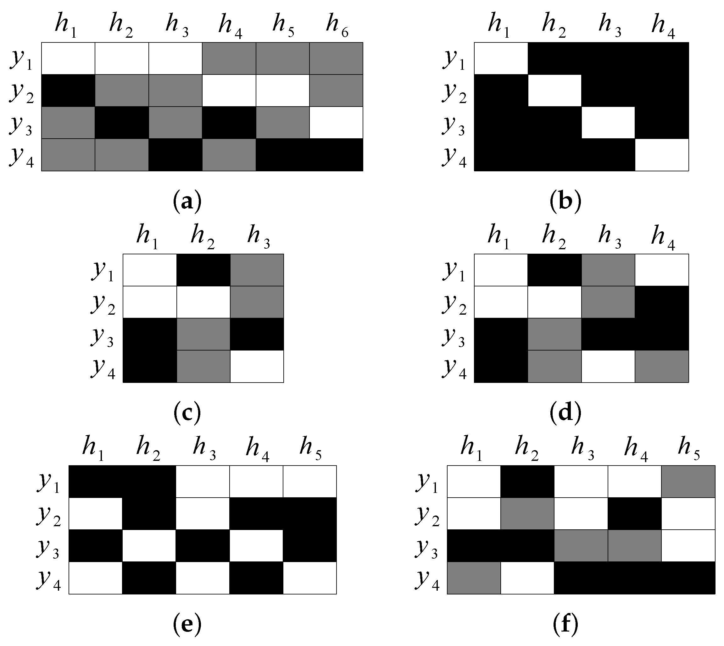
The general ECOC framework consists of two steps: coding and decoding. In the coding step, the ECOC coding matrix $\mathbf{M}\in {\{-1,0,1\}}^{C\times L}$ is first defined or learned from the training data, where each row of $\mathbf{M}$ is the codeword of a class, each column corresponds to a binary classifier (dichotomizer), L is the length of the codewords, C is the number of classes, symbol ‘1’ indicates a positive class, ‘−1’ indicates a negative class, and ‘0’ indicates the class that can be neglected during training the binary classifiers. Subsequently, the binary classifiers (dichotomizers) are trained according to the partition of the classes in each column of $\mathbf{M}$. Figure 1 shows some coding matrices encoded with different coding strategies. The white grids are coded by 1, the dark grids are coded by −1, and the gray grids are coded by 0. In the decoding step, the test data are predicted based on an adopted decoding strategy.

Applying a decoding strategy on the outputs of the binary classifier, the ECOC framework can be used for multi-class learning; meanwhile, applying the sigmoid function on the values of the discriminant functions of the binary classifiers, ECOC can be used for representation learning [6]. This is also the foundation of our DeepECOCs model. Specifically, to speed up the training of the binary classifiers in the ECOC modules of DeepECOC, we employ the online SVMs as binary classifiers [45].

3.2. Incremental Support Vector Machines (Incremental SVMs)

The Karush–Kuhn–Tucker (KKT) condition is a necessary and sufficient condition for determining whether a certain point of the convex function is an extreme point, and it has important applications in SVM.

3.2.1. KKT Conditions

To take the probabilistic outputs of the base classifiers as new representations of data, we adopt linear support vector machines (linear SVMs) as the binary classifiers (dichotomizers), which solve a quadratic programming problem

$$\begin{array}{ccc}\hfill & & \underset{\mathbf{w},b,{\xi }_i}{min}J\left(\mathbf{w}\right)=\frac{1}{2}{\parallel \mathbf{w}\parallel }^2+\lambda \sum _{i=1}^N{\xi }_i\hfill \\ & s.t.& y_{i}f\left({\mathbf{x}}_i\right)\ge 1-{\xi }_i,{\xi }_i\ge 0,i=1,\dots ,N\hfill \end{array}$$

(1)

where $\mathbf{w}$ and b are the coefficients and bias of the binary classifier, $y_i\in \{+1,-1\}$, ${\xi }_i$’s are the slack variables, and N is the number of the training data.

In the real world applications, the original sample space may not have a hyperplane that correctly divides the two types of samples. This is the need to use a kernel function to map samples from the original space to a higher dimensional feature space.

In order to overcome the limitation of off-line binary classifiers in ECOC framework, we use online SVM as binary classifiers [45] and apply it in our experiments. We rewrite the Problem (1) in a Lagrange form,

$$\underset{0\le {\alpha }_i\le C}{min}:J\left(\mathbf{w}\right)=\frac{1}{2}\sum _{i,j}{\alpha }_i{Q}_{ij}{\alpha }_j-\sum _i{\alpha }_i+b\sum _i{y}_i{\alpha }_i$$

(2)

where Q is a symmetric matrix $Q_{ij}=y_i{y}_{j}k({\mathbf{x}}_i,{\mathbf{x}}_j)$, and ${\alpha }_i$ is the Lagrange multiplier. The first-order conditions on $J\left(\mathbf{w}\right)$ reduce to the KKT conditions:

$$\begin{array}{cc}\hfill g_i=\frac{\partial J\left(\mathbf{w}\right)}{\partial {\alpha }_i}& ={\displaystyle \sum _j}{Q}_{ij}{\alpha }_j+y_{i}b-1\hfill \\ \hfill \hspace{1em}\hspace{1em}\hspace{1em}\hspace{1em}\hspace{1em}\hspace{1em}\hspace{1em}\hspace{1em}\hspace{1em}\hspace{1em}\hspace{1em} & =y_{i}f\left({\mathbf{x}}_i\right)-1\left\{\begin{array}{cc}>0;\hfill & {\alpha }_i=0\hfill \\ =0;\hfill & 0<{\alpha }_i<C\hfill \\ \le 0;\hfill & {\alpha }_i=C\hfill \end{array}\right.\hfill \end{array}$$

(3)

$$\begin{array}{ccc}\hfill \frac{\partial J\left(\mathbf{w}\right)}{\partial b}& =& \sum _j{y}_j{\alpha }_j=0\hfill \end{array}$$

(4)

The goal of incremental SVM is to preserve the KKT conditions for all previous training data when we add the unlearned examples into the solution. Based on the partial derivatives $g_i$, the training examples can be partitioned into three different categories: the set $\mathcal{S}$ of support vectors on the margin ($g_i=0$), the set $\mathcal{E}$ of error support vectors violating the condition ($g_i<0$), and the remaining set $\mathcal{R}$ of (ignored) vectors.

3.2.2. Incremental Learning Procedure

Let a be a new training sample, $X:X^{l+1}=X^l\cup a$. The incremental learning procedure is described as follows:

(1)

Initialize ${\alpha }_a$ to 0, then calculate $g_a$;

(2)

If $g_a>0$, terminate (a is not a margin or error vector);

(3)

If $g_a\le 0$, apply the largest possible increment ${\alpha }_a$ so that one of the following conditions occurs:

(a)

$g_a=0$: add a to margin set $\mathcal{S}$, terminate;

(b)

${\alpha }_a=C$: add a to error set $\mathcal{E}$, terminate;

(c)

Elements of $X^{l+1}$ migrate across $\mathcal{S}$, $\mathcal{E}$ and $\mathcal{R}$; update membership of elements, and if $\mathcal{S}$ changes, update $\mathcal{R}$ accordingly.

3.3. DeepECOCs

To combine the advantages of ECOC and deep learning algorithms, we build the DeepECOC architecture as follows

$$\mathbf{x}\stackrel{q_D}{\to }\tilde{\mathbf{x}}\underset{{\mathbf{b}}^1}{\overset{{\mathbf{W}}^1}{\to }}{\mathbf{z}}^1\underset{{\mathbf{b}}^2}{\overset{{\mathbf{W}}^2}{\to }}\cdots \underset{{\mathbf{b}}^{n-1}}{\overset{{\mathbf{W}}^{n-1}}{\to }}{\mathbf{z}}^{n-1}\stackrel{softmax}{\to }\mathbf{y},$$

(5)

where the first step makes the clean input $\mathbf{x}\in {[0,1]}^d$ partially destroyed by means of a stochastic mapping $\tilde{\mathbf{x}}\sim q_D(\tilde{\mathbf{x}}\mid \mathbf{x})$. In the corrupting process, we set a parameter called the denoising rate $\nu$. For each input $\mathbf{x}$, a fixed number $\nu d$ of components are chosen at random, and their value is forced to 0, while the others are left untouched. This operation makes the model more robust and prevents the overfitting problem in most cases [27]. Subsequently, the “corrupted“ data are taken as inputs for the DeepECOCs model. ${\mathbf{W}}^1$ and ${\mathbf{b}}^1$ are the weight matrix and bias vector learned from the first ECOC module. The output of the first hidden layer is denoted as

$${\mathbf{z}}^1=s({\left({\mathbf{W}}^1\right)}^T\mathbf{x}+{\mathbf{b}}^1),$$

(6)

where $s(·)$ is the sigmoid activation function $s\left(x\right)=\frac{1}{1+e^{-x}}$. From the second layer to the $(n-1)$-th layer, we use the stacked ECOC modules to learn the weight matrices and biases, which can be considered as weights between two successive layers. Similarly, we use the output of the $k-1$-th layer as the input of the k-th layer,

$${\mathbf{z}}^k=s({\left({\mathbf{W}}^k\right)}^T{\mathbf{z}}^{k-1}+{\mathbf{b}}^k).$$

(7)

Here, ${\mathbf{z}}^k$ can be viewed as an approximate posterior probability and new representation of the input datum $\mathbf{x}$.

For example, if we adopt the OneVsAll coding strategy for the stacked ECOC modules, we first define the coding matrix ${\mathbf{M}}^{C\times C}$, where C is the number of classes. Then, we can train C incremental SVM classifiers to obtain the weight matrix $\mathbf{W}=\{{\mathbf{w}}_1,\dots ,{\mathbf{w}}_i,\dots ,{\mathbf{w}}_C\}$ and the bias $\mathbf{b}=\{b_1,\dots ,b_i,\dots ,b_C\}$. Next, we calculate the output of the first layer by using Equation (6). Subsequently, we repeat this process layer by layer to build the DeepECOCs model. It is obvious that, if we adopt different coding strategies, we can obtain different kinds of DeepECOC architectures.

For the last layer of DeepECOCs, we employ the softmax regression for the multi-class learning. Its cost function is defined as

$$J\left(\mathbf{w}\right)=-\frac{1}{N}(\sum _{i=1}^N\sum _{j=1}^K\mathbf{I}(y_i=j)log\frac{exp\left({\mathbf{w}}_j^T{\mathbf{z}}_i^{n-1}\right)}{{\sum }_{l=1}^{K}exp\left({\mathbf{w}}_l^T{\mathbf{z}}_i^{n-1}\right)}),$$

(8)

where $\mathbf{I}\left(x\right)$ is the indicator function, and $\mathbf{I}\left(x\right)=1$ if x is true, else $\mathbf{I}\left(x\right)=0$. $y_i$ is the label corresponding to ${\mathbf{x}}_i$. It is easy to compute the probability that ${\mathbf{x}}_i$ is classified to class j,

$$p(y_i=j|{\mathbf{x}}_i,\mathbf{w})=\frac{exp\left({\mathbf{w}}_j^T{\mathbf{z}}_i^{n-1}\right)}{{\sum }_{l=1}^{K}exp\left({\mathbf{w}}_l^T{\mathbf{z}}_i^{n-1}\right)}.$$

(9)

Taking derivatives, one can show that the gradient of $J\left(\mathbf{w}\right)$ with respect to $\mathbf{w}$ is,

$$\nabla J\left(\mathbf{w}\right)=-\frac{1}{N}\sum _{i=1}^N\left[{\mathbf{x}}_i(\mathbf{I}(y_i=j)-p(y_i=j|{\mathbf{x}}_i,\mathbf{w}))\right].$$

(10)

After the initialization step, we use back propagation [46] to fine-tune the whole architecture. In the fine-tuning process, we apply the dropout technique for regularization [47]. It is a very efficient way to perform model averaging with neural networks. Through the above processes, we can finally obtain the DeepECOCs model, which is robust and easy to be applied to multi-class learning tasks. In summary, we show the training process of our DeepECOCs framework in Algorithm 1.

Note that DeepECOCs have some important advantages. Firstly, unlike previous deep learning algorithms, such as AE, DAE and DBNs, DeepECOCs are built with the ECOC modules and initialized in a supervised learning fashion. Secondly, if we adopt ternary coding strategies, due to the merit of ECOC, the weights can be learned using only part of the training data. Thirdly, in contrast to the learning of the weight matrices in previous deep learning models, the binary classifiers in each ECOC module can be learned in parallel, which may greatly speed up the learning of DeepECOCs.

Algorithm 1 The training procedure of DeepECOCs; L is the number of layers, I-SVM($\mathbf{x},\mathbf{y}$) is the incremental SVM binary classifier, $s\left(x\right)$ is the sigmoid function, and $\mathrm{softmax}\left(\mathbf{x}\right)$ is the softmax function.

Require:

The set of training samples $\mathbf{X}=\{{\mathbf{x}}_1,\dots ,{\mathbf{x}}_j,\dots ,{\mathbf{x}}_n\}$;

The labels corresponding to training samples $\mathbf{y}=\{y_1,\dots ,y_j,\dots ,y_n\}$.

Ensure:

Parameters $\mathbf{W}$ and $\mathbf{b}$.

1: Initialize the first layer input ${\mathbf{Z}}^1=\mathbf{X}$;

2: for $i=1$ to $L-1$ do

3:  Initialize the weights and bias of i-th ECOC module;

4:  ${\mathbf{W}}^i=\mathbf{0},{\mathbf{b}}^i=\mathbf{0}$;

5:  Pre-train process (ECOC coding step):

6:  (1) Learn the ECOC matrix with a coding strategy, and obtain $\mathbf{M}\in {\{-1,1\}}^{C\times P}$ (binary case) or $\mathbf{M}\in {\{-1,0,1\}}^{C\times P}$ (ternary case);

7:  (2) Train the incremental SVM binary classifiers according to $\mathbf{M}$:

8:  for $k=1$ to P do

9:   $({\alpha }_k,b_k^i)\leftarrow$ I-SVM$({\mathbf{Z}}^i,\mathbf{y})$;

10:  ${\mathbf{w}}_k^i={\sum }_{j=1}^N{\alpha }_j{y}_j{\mathbf{Z}}_j^i$;

11:   end for

12:   ${\mathbf{W}}^i=\{{\mathbf{w}}_1^i,\dots ,{\mathbf{w}}_k^i,\dots ,{\mathbf{w}}_P^i\}$;

13:   ${\mathbf{b}}^i=\{b_1^i,\dots ,b_k^i,\dots ,b_P^i\}$;

14:   ${\mathbf{z}}^{i+1}=s({\left({\mathbf{W}}^i\right)}^T{\mathbf{z}}^i+{\mathbf{b}}^i)$;

15: end for

16: ${\mathbf{z}}^L=\mathrm{softmax}\left({\mathbf{z}}^{L-1}\right)$.

17: Use the back-propagation algorithm for fine-tuning.

18: return $\mathbf{W}=\left\{{\mathbf{W}}^i\right\}$ and $\mathbf{b}=\left\{{\mathbf{b}}^i\right\}$, $i=1,\dots ,L-1$.

3.4. Combining Convolutional Neural Networks (CNNs) with DeepECOCs

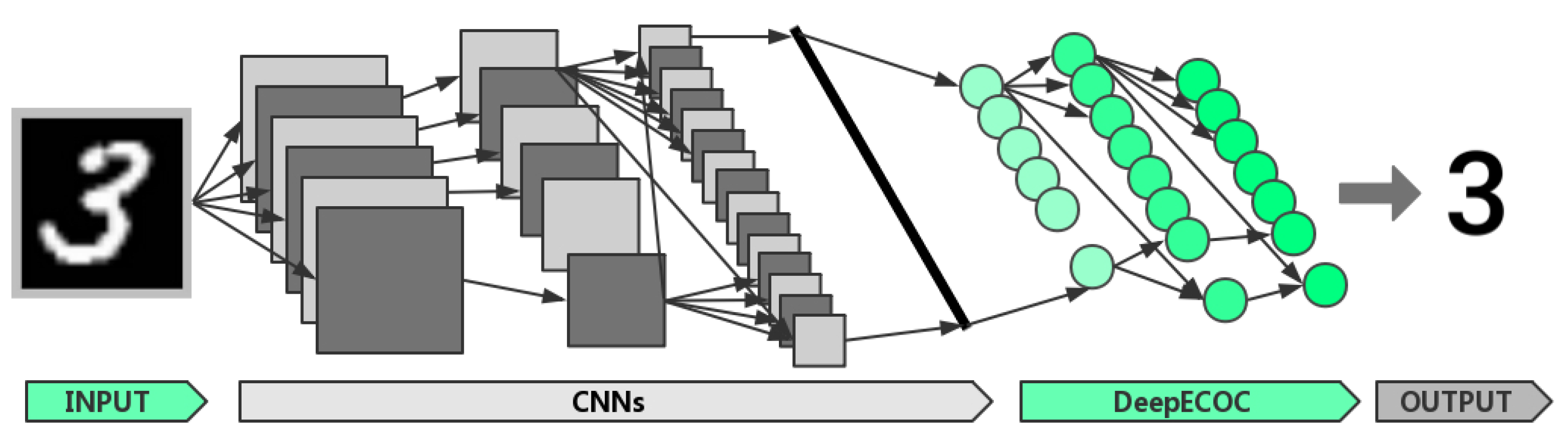
CNNs can effectively extract features from images and videos [48,49], while DeepECOCs can be used as a strong and flexible classifier. Here, we construct a new deep architecture to integrate the advantages of CNNs and DeepECOCs. Figure 2 illustrates such a deep architecture. In the next section, we demonstrate that this architecture can improve the accuracy of the original CNNs.

The training process of this combined neural architecture consists of three steps. Firstly, we train the original CNNs as usual. Secondly, we take the output of the fully connected layer before the classifier as the input of DeepECOCs, and train DeepECOCs. Finally, we fine-tune the whole network by training it for a few epochs.

4. Experiments

To evaluate the effectiveness of the proposed method, DeepECOCs, we conducted 6 experiments. In the first one, we compared DeepECOCs with some deep learning models and a single-layer ECOC framework on 16 small and medium data sets from the UCI machine learning repository (http://archive.ics.uci.edu/ml/ (accessed on 19 October 2023)). In the second one, we used the USPS handwritten digits data set (https://www.csie.ntu.edu.tw/~cjlin/libsvmtools/datasets/multiclass.html#usps (accessed on 19 October 2023)) and tested DeepECOCs with a different number of hidden layers. In the third one, we used the MNIST data set (http://yann.lecun.com/exdb/mnist/ (accessed on 19 October 2023)) to further demonstrate the effectiveness of DeepECOCs on handwritten digits recognition tasks. In the fourth one, to demonstrate the effectiveness of DeepECOCs on action recognition applications, we applied it to the CMU motion capture data set (http://mocap.cs.cmu.edu/ (accessed on 19 October 2023)). For all the data sets we mentioned above, to equate the scales of the data features and ease the training of the base classifiers, the features were normalized within $[0,1]$ [50]. In the fifth part, the CIFAR-10 data set (http://www.cs.toronto.edu/~kriz/cifar.html (accessed on 19 October 2023)) was used to demonstrate the effectiveness of DeepECOCs on image classification tasks compared with the related deep neural networks. Finally, we tested DeepECOCs on improving the effectiveness of CNNs. In the following, we present the experimental results in detail.

4.1. Classification on 16 UCI Data Sets

In these experiments, we first compared the effect of using traditional SVMs against that using online SVMs to build the ECOC framework. The detail of the UCI data sets is shown in

Table 1. Details of the UCI data sets (I: Instances; A: attributes; C: classes).

Problem	♯ of I	♯ of A	♯ of C	Problem	♯ of I	♯ of A	♯ of C
Dermatology	366	34	6	Yeast	1484	8	10
Iris	150	4	3	Satimage	6435	36	7
Ecoli	336	8	8	Letter	20,000	16	26
Wine	178	13	3	Pendigits	10,992	16	10
Glass	214	9	7	Segmentation	2310	19	7
Thyroid	215	5	3	Optdigits	5620	64	10
Vowel	990	10	11	Shuttle	14,500	9	7
Balance	625	4	3	Vehicle	846	18	4

. We used 4 coding strategies, including one-versus-all, one-versus-one, DECOC and ECOCONE (initialized by one-versus-one). The linear loss-weighted (LLW) decoding strategy was applied for all the methods [9]. We chose SVMs with RBF kernel function as the traditional binary classifier (for short, LibSVM) [17]. The results based on the 10-fold cross validation are shown in

Table 2. Classification accuracy on the 16 UCI data sets obtained by comparing LibSVM and incremental SVM. The best results for each scenario are highlighted in bold face.

Problem	OneVsOne		OneVsAll		DECOC		ECOCONE
	LibSVM	I-SVM	LibSVM	I-SVM	LibSVM	I-SVM	LibSVM	I-SVM
Dermatology	0.9671	0.9770	0.7928	0.9605	0.9671	0.9638	0.9671	0.9770
Iris	0.9333	0.9333	0.7030	0.7030	0.9333	0.9333	0.9333	0.9333
Ecoli	0.5944	0.6507	0.3940	0.4553	0.5281	0.5828	0.5944	0.6556
Wine	0.9892	0.9892	0.9731	0.9731	0.9892	0.9731	0.9839	0.9892
Glass	0.4838	0.4189	0.3216	0.3270	0.2973	0.3486	0.3027	0.5378
Thyroid	0.5897	0.6239	0.5897	0.6239	0.5897	0.4017	0.5897	0.6239
Vowel	0.4187	0.4956	0.3953	0.6591	0.2736	0.3278	0.4476	0.4956
Balance	0.8927	0.8927	0.9042	0.9042	0.8927	0.8927	0.8927	0.8927
Yeast	0.4741	0.5744	0.2383	0.2760	0.3751	0.5693	0.4147	0.6000
Satimage	0.8361	0.8692	0.7620	0.8334	0.7411	0.8532	0.8305	0.8604
Letter	0.7443	0.8216	0.2166	0.4536	0.7530	0.8375	0.7440	0.8120
Pendigits	0.9688	0.9859	0.9021	0.9773	0.9065	0.9758	0.9691	0.9850
Segmentation	0.8595	0.8872	0.6187	0.6759	0.7969	0.6706	0.8601	0.8872
OptDigits	0.9492	0.9860	0.8866	0.9649	0.8793	0.9808	0.9492	0.9860
Shuttle	0.9178	0.9475	0.8312	0.9034	0.8352	0.9407	0.9179	0.9532
Vehicle	0.6324	0.7595	0.7378	0.4892	0.6054	0.7243	0.6324	0.7595

. We can observe that incremental SVM performs better than LibSVM when applied to build the ECOC framework in most cases. Moreover, it is easy to handle the relative large-scale applications.

Then, we compared DeepECOCs with AE [26], DAE [27] and the single-layer ECOC framework [9]. We built our DeepECOCs with different coding design methods. They were one-versus-all, one-versus-one, discriminant ECOC (DECOC) and ECOC optimizing node embedding (ECOCONE). Here, because the ECOCONE’s initial codings were different (initialized by one-versus-all, one-versus-one and DECOC), the coding strategies of DeepECOCs had 6 types. In our experiments, we adopted 3 hidden layers DeepECOCs with 0.1 denoising rate and 0.1 dropout rate,

$$\mathbf{x}\stackrel{q_D}{\to }\tilde{\mathbf{x}}\underset{{\mathbf{b}}^1}{\overset{{\mathbf{W}}^1}{\to }}{\mathbf{z}}^1\underset{{\mathbf{b}}^2}{\overset{{\mathbf{W}}^2}{\to }}{\mathbf{z}}^2\underset{{\mathbf{b}}^3}{\overset{{\mathbf{W}}^3}{\to }}{\mathbf{z}}^3\stackrel{softmax}{\to }\mathbf{y}.$$

(11)

For the fine-tuning process, we used the stochastic gradient descent algorithm. The learning rate and epoches for different data sets were given in

Table 3. Details of the learning rate $\eta$ and epoch on the UCI data sets.

Problem	$\mathit{\eta }$	Epoch	Problem	$\mathit{\eta }$	Epoch
Dermatology	0.1	2000	Yeast	0.01	4000
Iris	0.1	400	Satimage	0.01	4000
Ecoli	0.1	2000	Letter	0.01	8000
Wine	0.1	2000	Pendigits	0.01	2000
Glass	0.01	4000	Segmentation	0.01	8000
Thyroid	0.1	800	Optdigits	0.01	2000
Vowel	0.1	4000	Shuttle	0.1	2000
Balance	0.1	4000	Vehicle	0.1	4000

. The autoencoder and denoising autoencoder’s architectures were same as the DeepECOCs with ECOCONE (initializing by one-versus-one) coding design method. For the single-layer ECOC framework, we chose the best results from [9] as the compared results. The average classification accuracy and standard deviation based on a 10-fold cross validation were reported.

Table 4. Classification accuracy and standard deviation obtained by DeepECOCs and the compared approaches on the 16 UCI data sets. V1∼V6 represents DeepECOCs with different coding strategies, including OneVsOne, OneVsAll, DECOC and ECOCONE (initialized by OneVsOne, OneVsAll and DECOC). The best results are highlighted in boldface.

Problem	Single	AE	DAE	V1	V2	V3	V4
Dermatology	0.9513	0.9429 ± 0.0671	0.9674 ± 0.0312	0.9731 ± 0.0314	0.8852 ± 0.0561	0.9722 ± 0.0286	0.8834  ± 0.0349
Iris	0.9600	0.9600 ± 0.0562	0.9333 ± 0.0889	0.8818 ± 0.0695	0.8137 ± 0.0768	0.9667 ± 0.0471	0.9667 ± 0.0471
Ecoli	0.8147	0.7725 ± 0.0608	0.8000 ± 0.0362	0.8275  ± 0.0427	0.7868 ± 0.0633	0.9102 ± 0.0701	0.9183 ± 0.0611
Wine	0.9605	0.9765 ± 0.0264	0.9563 ± 0.0422	0.9063  ± 0.0793	0.9625 ± 0.0604	0.9875 ± 0.0264	0.9625 ± 0.0437
Glass	0.6762	0.6669 ± 0.1032	0.6669 ± 0.0715	0.7563  ± 0.0653	0.6875  ± 0.0877	0.8013  ± 0.0476	0.7830  ± 0.0893
Thyroid	0.9210	0.9513 ± 0.0614	0.9599 ± 0.0567	0.8901 ± 0.1177	0.9703 ± 0.0540	0.9647 ± 0.0431	0.9560 ± 0.0633
Vowel	0.7177	0.6985 ± 0.0745	0.7101 ± 0.0756	0.7020 ± 0.0529	0.6563 ± 0.0721	0.7628 ± 0.0716	0.6874 ± 0.0438
Balance	0.8222	0.8036 ± 0.0320	0.8268 ± 0.0548	0.8528 ± 0.0534	0.8108 ± 0.0634	0.8879 ± 0.1331	0.9090 ± 0.0438
Yeast	0.5217	0.5641 ± 0.0346	0.5891 ± 0.0272	0.5861 ± 0.0318	0.5368 ± 0.0582	0.6080 ± 0.0385	0.5968 ± 0.0378
Satimage	0.8537	0.8675 ± 0.0528	0.8897 ± 0.0304	0.8763 ± 0.0576	0.8238 ± 0.0453	0.8977 ± 0.0752	0.9108 ± 0.0483
Letter	0.9192	0.9234 ± 0.0547	0.9381 ± 0.0641	0.9498 ± 0.0587	0.9322 ± 0.0251	0.9553 ± 0.0327	0.9465 ± 0.0414
Pendigits	0.9801	0.9831 ± 0.0123	0.9886 ± 0.0034	0.9828 ± 0.0047	0.9768 ± 0.0034	0.9917 ± 0.0021	0.9817 ± 0.0082
Segmentation	0.9701	0.9584 ± 0.0317	0.9596 ± 0.0211	0.9683 ± 0.0412	0.9567 ± 0.0527	0.9757 ± 0.0296	0.9724 ± 0.0371
Optdigits	0.9982	0.9785 ± 0.0101	0.9856 ± 0.0088	0.9882 ± 0.0104	0.9845 ± 0.0122	0.9934 ± 0.0027	0.9901 ± 0.0033
Shuttle	0.9988	0.9953 ± 0.0012	0.9976 ± 0.0014	0.9991 ± 0.0017	0.9983 ± 0.0018	0.9996 ± 0.0012	0.9993 ± 0.0010
Vehicle	0.7315	0.6987 ± 0.0521	0.7348 ± 0.0454	0.7128 ± 0.0384	0.6624 ± 0.0472	0.7466 ± 0.0481	0.7097 ± 0.0521
Mean rank	5.2500	6.3125	4.9375	4.3125	7.0625	1.4375	3.1875

shows the average classification accuracy and standard deviation on the 16 UCI data sets. Except for the OptDigits data set, DeepECOCs consistently achieved the best results compared with autoencoder, denoising autoencoder and single-layer ECOC framework. On the OptDigits data set, indeed, DeepECOCs achieved a comparative result with the single-layer ECOC framework. In addition, DeepECOCs with an ECOCONE coding strategy achieved the best results in most cases. From the mean rank value, we can observe that DeepECOC with an ECOCONE strategy (initialized by one-versus-one and DECOC) far surpasses other methods.

4.2. Classification on the USPS Data Set

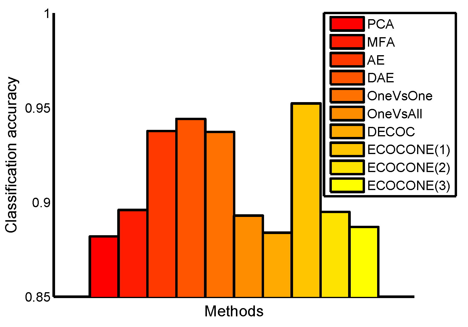
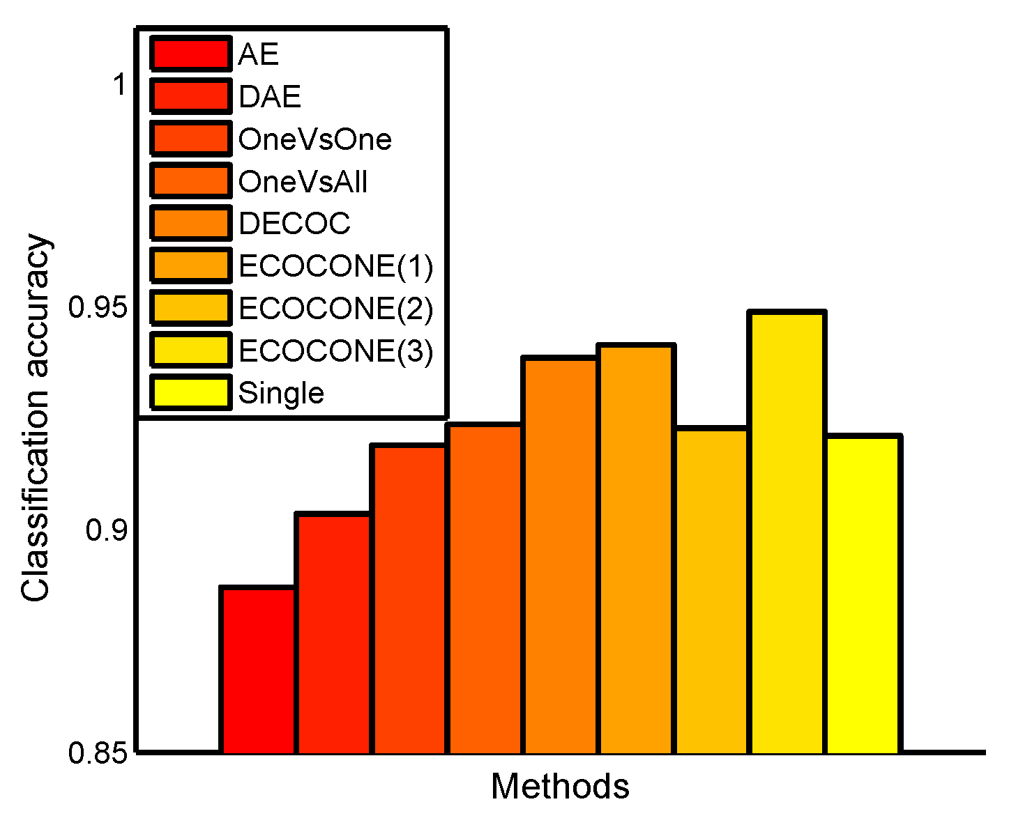
The USPS handwritten digits data set includes 7291 training samples and 2007 test samples from 10 classes with 256 dimensional features. Our experiments on this data set were divided into 2 parts. Firstly, we compared DeepECOCs with two traditional feature learning models (including a principal component analysis (PCA) [51] and marginal Fisher analysis (MFA) [52]), AE, DAE and single-layer ECOC framework. For MFA, the number of nearest neighbors for constructing the intrinsic graph was set to 5, while that for constructing the penalty graph was set to 15. For DeepECOCs, we also used 6 coding design methods, as in the previous experiments. We used a batch gradient descent for the fine-tuning process; the batch size was set to 100, the learning rate was set to 1, the number of epoch was set to 40,000 and the denoising rate and dropout rate were set to 0.1. We also used the incremental SVMs with an RBF kernel as base classifiers. For the single-layer ECOC framework, we adopted ECOCONE (initializing by one-versus-one) as the coding design method and linear loss-weighted (LLW) decoding strategy. The experimental results are shown in Figure 3.

From Figure 3, we can observe that DeepECOCs with the ECOCONE (initializing by one-versus-one) coding strategy achieved the best result among other methods, including traditional feature learning models, existing deep learning methods and a single-layer ECOC framework. However, if we used other coding design strategies (except ECOCONE initialized by one-versus-one), the DeepECOCs did not outperform an autoencoder and denoising autoencoder.

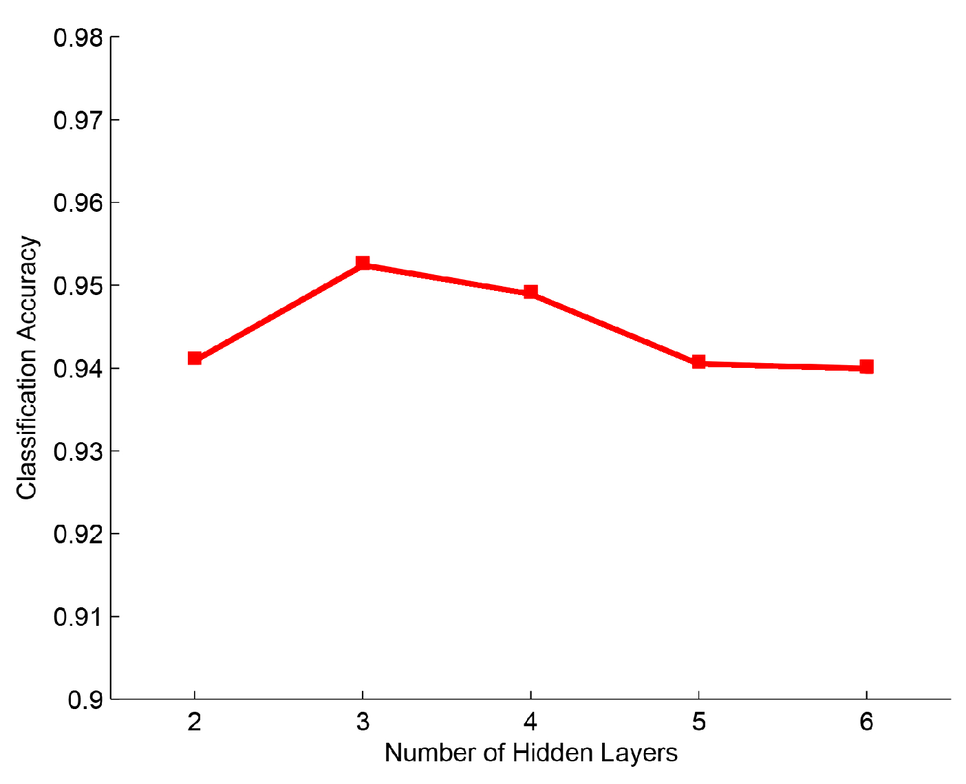
In the second part, we evaluated DeepECOCs with a different number of hidden layers, and we used 2 to 6 hidden layers in our experiments. The parameter settings were the same as in the first part. Figure 4 shows the experimental results. We can observe that DeepECOCs obtained the best result when adopting 3 hidden layers. When the number of hidden layers was less than 3, the accuracies obtained by DeepECOCs increased, and the number of the hidden layers increased. When with the number of the hidden layers was more than 3, the performance of DeepECOCs decreased.

4.3. Classification on the MNIST Data Set

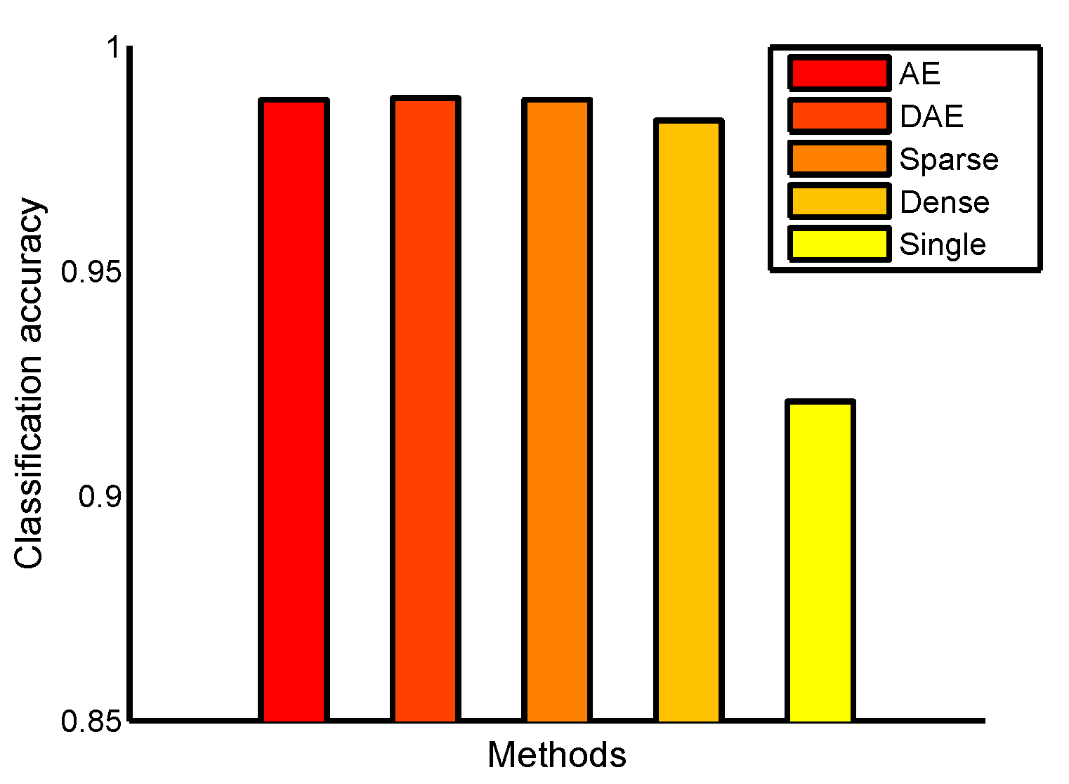
MNIST includes a training set of 60,000 samples and a test set of 10,000 samples with 784 dimensional features. We designed an architecture for the autoencoder, denoising autoencoder and DeepECOCs. The architecture is 784-$Z_1$-$Z_2$-$Z_3$-10. Here, $Z_i$ denotes the hidden layer learned from some coding strategies. We designed this architecture because we wanted to make the autoencoder and denoising autoencoder have the same structures as DeepECOCs. In order to make DeepECOCs adapt to this structure, we used the dense and sparse coding design methods that controlled the codeword length. The denoising rate and dropout rate were set to 0.1, the batch size was set to 100, the learning rate was set to 0.01, and the number of epochs was set to 80,000. Figure 5 shows the comparison results. We can observe that DeepECOCs achieve comparable results with the autoencoder and denoising autoencoder, but perform better than the single-layer ECOC framework.

Figure 6 shows the experimental results with a new deep architecture. We can observe that DeepECOCs outperform other compared methods. In addition, DeepECOCs with the ECOCONE (initialized by DECOC) coding strategy achieved the best result. Note that, in this scenario, all the deep networks shared the same architecture.

4.4. Classification on the CMU Mocap Data Set

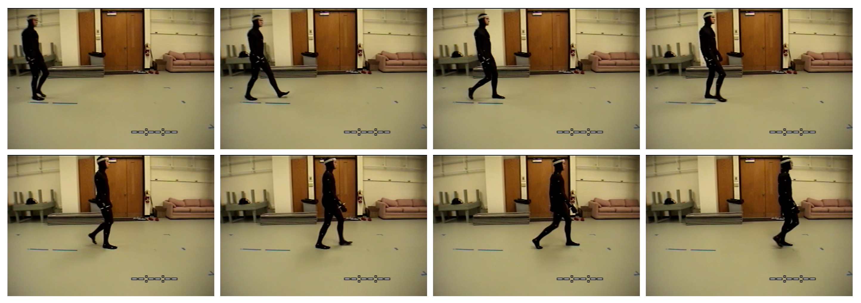
The CMU mocap data set includes three categories, namely, jumping, running and walking. We chose 49 video sequences of four subjects. For each sequence, the features were generated using Lawrence’s method [53], with a dimensionality of 93. Figure 7 shows one video sequence from the CMU mocap data set. We used 3 hidden layers for all deep learning methods. The learning rate was set to 0.1 and the epoch was set to 400. The other parameters were the same as in the previous experiments. The average classification accuracy based on the 10-fold cross validation are reported in

Table 5. The classification accuracy on the CMU mocap data set. The best results for each scenario are highlighted in bold face.

Problem	AE	DAE	V1	V2	V4	V5
CMU	0.6171	0.6422	0.8030	0.6364	0.7652	0.6030

.

From Table 5, we can easily observe that DeepECOCs achieved the best results in the CMU mocap data set, and DeepECOCs with a one-versus-one coding strategy far surpass other methods.

4.5. Classification on the CIFAR-10 Data set

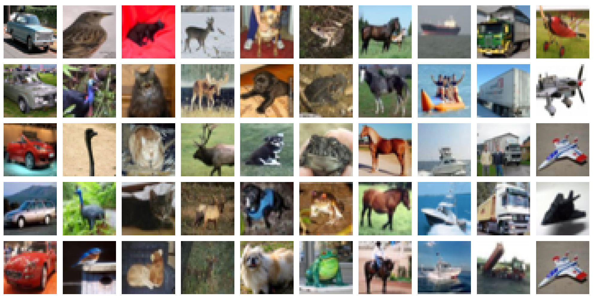
The CIFAR-10 data set consists of 60,000 $32\times 32$ colour images in 10 classes, with 6000 images per class. There are 50,000 training images and 10,000 test images. Figure 8 shows some samples from the 10 categories. For the purpose of reducing computational cost, we attempted to create a compact representation of the data using an efficient local binary patterns algorithm. As a result, the representation of dimensionality 36 and 256 were adopted and the data were normalized to [0, 1], as well. We also used 3 hidden layers for all deep learning methods. The learning rate was set to 0.1, and the epoch was set to 4000. Other parameters were the same as the previous experiments. The classification accuracy are reported in

Table 6. The classification accuracy on the CIFAR-10 data set. The best results for each scenario are highlighted in bold face.

Problem	AE	DAE	V1	V2
CIFAR(36)	0.3501	0.3678	0.4530	0.3895
CIFAR(256)	0.4352	0.4587	0.4936	0.4521
Problem	V3	V4	V5	V6
CIFAR(36)	0.4031	0.5089	0.4517	0.4752
CIFAR(256)	0.5236	0.5588	0.4589	0.5224

.

From Table 6, we can observe that DeepECOCs achieved the best results. Since we compressed the data using the local binary pattern algorithm, the results are not comparable with the state-of-the-art results. However, for the compared methods, they are fair. In this case, DeepECOCs with the ECOCONE (initialized by one-versus-one) coding strategy achieved better results than the autoencoder and denoising autoencoder. This means that DeepECOCs are general models to handle real world applications and can often achieve desirable results. In addition, from all of the above experiments, we can basically conclude that DeepECOCs with the ECOCONE (initialized by one-versus-one) coding strategy often perform very well.

4.6. Combining CNNs with DeepECOCs

In this experiment, we combined CNNs and DeepECOCs to improve the performance of the original CNNs. The CIFAR-10 data set was used. We first trained a ResNet for 200 epochs, as the baseline model (denoted as ResNet-baseline). Then, we trained it from scratch for 50 epochs, and subsequently, used the flattened output of the last convolutional layer to train DeepECOCs. Here, the architecture of DeepECOCs was m-505-225-220-10, where m was the dimension of the flattened features, and the coding strategy of the ECOC modules was the dense coding. Finally, the whole CNNs+DeepECOCs model (denoted as ResNet-DeepECOCs) was fine-tuned for 80 epochs.

Table 7. The classification accuracy obtained on the CIFAR-10 data set. The best result is highlighted in boldface.

Methods	ResNet-Baseline	ResNet-DeepECOCs
Accuracy	0.9098	0.9208

shows the obtained results. As we can observe, DeepECOCs improve the performance of the original CNNs.

5. Conclusions

In this paper, we propose a novel deep learning model, called deep error-correcting output codes (DeepECOCs). DeepECOCs extend the traditional ECOC framework in a deep architecture fashion. Extensive experiments on 16 data sets from the UCI machine learning repository, the USPS and MNIST handwritten digits, the CMU motion capture data set and the CIFAR-10 data set, demonstrate the superiority of DeepECOCs over the related ECOC, feature learning and deep learning methods.

In future work, we would like to develop new coding strategies that may improve the learnability of DeepECOCs on broader applications than we have tested in this paper. Moreover, for the training of the base classifiers, parallel computing is one way to improve the learning efficiency. Hence, we will implement parallel computing to speed up the optimization of DeepECOCs. Additionally, we plan to combine DeepECOCs with Transformer models [31], using the attention mechanism of Transformer models to extract useful features for DeepECOCs, in contrast to the combination of DeepECOCs and CNNs introduced in Section 3.4. In this case, we may achieve the state-of-the-art learning results on different tasks, such as object recognition and detection.

References

- Dietterich, T.G.; Bakiri, G. Solving multiclass learning problems via error-correcting output codes. J. Artif. Intell. Res. 1995, 2, 263–286. [Google Scholar] [CrossRef]
- Breiman, L. Random Forests. Mach. Learn. 2001, 45, 5–32. [Google Scholar] [CrossRef]
- Schapire, R.E. A Brief Introduction to Boosting. IJCAI 2010, 14, 377–380. [Google Scholar]
- Kumar, A.; Kaur, A.; Singh, P.; Driss, M.; Boulila, W. Efficient Multiclass Classification Using Feature Selection in High-Dimensional Datasets. Electronics 2023, 12, 2290. [Google Scholar] [CrossRef]
- Saeed, M.M.; Saeed, R.A.; Abdelhaq, M.; Alsaqour, R.; Hasan, M.K.; Mokhtar, R.A. Anomaly Detection in 6G Networks Using Machine Learning Methods. Electronics 2023, 12, 3300. [Google Scholar] [CrossRef]
- Zhong, G.; Liu, C.L. Error-correcting output codes based ensemble feature extraction. Pattern Recognit. 2013, 46, 1091–1100. [Google Scholar] [CrossRef]
- Ghani, R. Using error-correcting codes for text classification. In Proceedings of the ICML ’00: Seventeenth International Conference on Machine Learning, Stanford, CA, USA, 29 June–2 July 2000; pp. 303–310. [Google Scholar]
- Escalera, S.; Masip, D.; Puertas, E.; Radeva, P.; Pujol, O. Online error correcting output codes. Pattern Recognit. Lett. 2011, 32, 458–467. [Google Scholar] [CrossRef]
- Escalera, S.; Pujol, O.; Radeva, P. On the decoding process in ternary error-correcting output codes. IEEE Trans. Pattern Anal. Mach. Intell. 2010, 32, 120–134. [Google Scholar] [CrossRef]
- Nilsson, N.J. Learning Machines; McGraw-Hill: New York, NY, USA, 1965. [Google Scholar]
- Hastie, T.; Tibshirani, R. Classification by pairwise coupling. Ann. Stat. 1998, 26, 451–471. [Google Scholar] [CrossRef]
- Pujol, O.; Radeva, P.; Vitria, J. Discriminant ECOC: A heuristic method for application dependent design of error correcting output codes. IEEE Trans. Pattern Anal. Mach. Intell. 2006, 28, 1007–1012. [Google Scholar] [CrossRef]
- Escalera, S.; Pujol, O.; Radeva, P. ECOC-ONE: A novel coding and decoding strategy. In Proceedings of the ICPR, Hong Kong, China, 20–24 August 2006; Volume 3, pp. 578–581. [Google Scholar]
- Escalera, S.; Pujol, O.; Radeva, P. Separability of ternary codes for sparse designs of error-correcting output codes. Pattern Recognit. Lett. 2009, 30, 285–297. [Google Scholar]
- Allwein, E.L.; Schapire, R.E.; Singer, Y. Reducing multiclass to binary: A unifying approach for margin classifiers. J. Mach. Learn. Res. 2001, 1, 113–141. [Google Scholar]
- Freund, Y.; Schapire, R.E. Experiments with a new boosting algorithm. In Proceedings of the ICML, Machine Learning, Bari, Italy, 3–6 July 1996; Volume 96, pp. 148–156. [Google Scholar]
- Chang, C.C.; Lin, C.J. LIBSVM: A library for support vector machines. Acm Trans. Intell. Syst. Technol. 2011, 2, 27. [Google Scholar] [CrossRef]
- Han, K.; Wang, Y.; Chen, H.; Chen, X.; Guo, J.; Liu, Z.; Tang, Y.; Xiao, A.; Xu, C.; Xu, Y.; et al. A Survey on Vision Transformer. IEEE Trans. Pattern Anal. Mach. Intell. 2023, 45, 87–110. [Google Scholar] [CrossRef] [PubMed]
- Krizhevsky, A.; Sutskever, I.; Hinton, G. ImageNet classification with deep convolutional neural networks. In Proceedings of the Advances in Neural Information Processing Systems 25 (NIPS 2012), Lake Tahoe, NV, USA, 3–6 December 2012; pp. 1106–1114. [Google Scholar]
- Zhang, R.; Lin, L.; Zhang, R.; Zuo, W.; Zhang, L. Bit-scalable deep hashing with regularized similarity learning for image retrieval and person re-identification. IEEE Trans. Image Process. 2015, 24, 4766–4779. [Google Scholar] [CrossRef] [PubMed]
- Szegedy, C.; Liu, W.; Jia, Y.; Sermanet, P.; Reed, S.; Anguelov, D.; Erhan, D.; Vanhoucke, V.; Rabinovich, A. Going deeper with convolutions. In Proceedings of the CVPR, Boston, MA, USA, 7–12 June 2015; pp. 1–9. [Google Scholar]
- Hinton, G.; Deng, L.; Yu, D.; Dahl, G.E.; Mohamed, A.r.; Jaitly, N.; Senior, A.; Vanhoucke, V.; Nguyen, P.; Sainath, T.N.; et al. Deep neural networks for acoustic modeling in speech recognition: The shared views of four research groups. Signal Process. Mag. IEEE 2012, 29, 82–97. [Google Scholar] [CrossRef]
- Severyn, A.; Moschitti, A. Learning to rank short text pairs with convolutional deep neural networks. In Proceedings of the SIGIR ’15: 38th International ACM SIGIR Conference on Research and Development in Information, Santiago, Chile, 9–13 August 2015; pp. 373–382. [Google Scholar]
- Zheng, Y.; Cai, Y.; Zhong, G.; Chherawala, Y.; Shi, Y.; Dong, J. Stretching deep architectures for text recognition. In Proceedings of the 2015 13th International Conference on Document Analysis and Recognition (ICDAR), Tunis, Tunisia, 23–26 August 2015; pp. 236–240. [Google Scholar]
- Chitta, K.; Prakash, A.; Jaeger, B.; Yu, Z.; Renz, K.; Geiger, A. TransFuser: Imitation with Transformer-Based Sensor Fusion for Autonomous Driving. IEEE Trans. Pattern Anal. Mach. Intell. 2023, 45, 12878–12895. [Google Scholar] [CrossRef]
- Hinton, G.; Salakhutdinov, R. Reducing the dimensionality of data with neural networks. Science 2006, 313, 504–507. [Google Scholar] [CrossRef]
- Vincent, P.; Larochelle, H.; Bengio, Y.; Manzagol, P.-A. Extracting and composing robust features with denoising autoencoders. In Proceedings of the ICML ’08: 25th International Conference on Machine Learning, Helsinki, Finland, 5–9 July 2008; pp. 1096–1103. [Google Scholar]
- Mak, H.W.L.; Han, R.; Yin, H.H.F. Application of Variational AutoEncoder (VAE) Model and Image Processing Approaches in Game Design. Sensors 2023, 23, 3457. [Google Scholar] [CrossRef]
- Sharif, S.A.; Hammad, A.; Eshraghi, P. Generation of whole building renovation scenarios using variational autoencoders. Energy Build. 2021, 230, 110520. [Google Scholar] [CrossRef]
- Hinton, G.E.; Osindero, S.; Teh, Y.W. A fast learning algorithm for deep belief nets. Neural Comput. 2006, 18, 1527–1554. [Google Scholar] [CrossRef] [PubMed]
- Vaswani, A.; Shazeer, N.; Parmar, N.; Uszkoreit, J.; Jones, L.; Gomez, A.N.; Kaiser, L.U.; Polosukhin, I. Attention is All you Need. In Proceedings of the Advances in Neural Information Processing Systems 30: Annual Conference on Neural Information Processing Systems 2017, Long Beach, CA, USA, 4–9 December 2017; Volume 30. [Google Scholar]
- Dirgova Luptakova, I.; Kubovcik, M.; Pospichal, J. Wearable Sensor-Based Human Activity Recognition with Transformer Model. Sensors 2022, 22, 1911. [Google Scholar] [CrossRef] [PubMed]
- Zhao, X.; Zhang, S.; Shi, R.; Yan, W.; Pan, X. Multi-Temporal Hyperspectral Classification of Grassland Using Transformer Network. Sensors 2023, 23, 6642. [Google Scholar] [CrossRef] [PubMed]
- Breiman, L. Bagging Predictors. Mach. Learn. 1996, 24, 123–140. [Google Scholar] [CrossRef]
- Sabzevari, M.; Martínez-Muñoz, G.; Suárez, A. Vote-boosting ensembles. Pattern Recognit. 2018, 83, 119–133. [Google Scholar] [CrossRef]
- Claesen, M.; Smet, F.D.; Suykens, J.A.; Moor, B.D. EnsembleSVM: A library for ensemble learning using support vector machines. J. Mach. Learn. Res. 2014, 15, 141–145. [Google Scholar]
- Hu, C.; Chen, Y.; Hu, L.; Peng, X. A novel random forests based class incremental learning method for activity recognition. Pattern Recognit. 2018, 78, 277–290. [Google Scholar] [CrossRef]
- Sun, Y.; Tang, K.; Minku, L.; Wang, S.; Yao, X. Online Ensemble Learning of Data Streams with Gradually Evolved Classes. IEEE Trans. Knowl. Data Eng. 2016, 28, 1532–1545. [Google Scholar] [CrossRef]
- Wang, S.; Minku, L.L.; Yao, X. Resampling-Based Ensemble Methods for Online Class Imbalance Learning. IEEE Trans. Knowl. Data Eng. 2015, 27, 1356–1368. [Google Scholar] [CrossRef]
- Deng, L.; Platt, J.C. Ensemble deep learning for speech recognition. In Proceedings of the INTERSPEECH, Singapore, 14–18 September 2014; pp. 1915–1919. [Google Scholar]
- Zhou, X.; Xie, L.; Zhang, P.; Zhang, Y. An ensemble of deep neural networks for object tracking. In Proceedings of the 2014 IEEE International Conference on Image Processing (ICIP), Paris, France, 27–30 October 2014; pp. 843–847. [Google Scholar]
- Maji, D.; Santara, A.; Mitra, P.; Sheet, D. Ensemble of Deep Convolutional Neural Networks for Learning to Detect Retinal Vessels in Fundus Images. arXiv 2016, arXiv:1603.04833. [Google Scholar]
- Trigeorgis, G.; Bousmalis, K.; Zafeiriou, S.; Schuller, B. A deep semi-nmf model for learning hidden representations. In Proceedings of the ICML’14: 31st International Conference on International Conference on Machine Learning, Beijing, China, 21–26 June 2014; pp. 1692–1700. [Google Scholar]
- Sak, H.; Senior, A.; Beaufays, F. Long short-term memory recurrent neural network architectures for large scale acoustic modeling. In Proceedings of the INTERSPEECH, Singapore, 14–18 September 2014; pp. 338–342. [Google Scholar]
- Poggio, T.; Cauwenberghs, G. Incremental and decremental support vector machine learning. NIPS 2001, 13, 409. [Google Scholar]
- Rumelhart, D.E.; Hinton, G.E.; Williams, R.J. Learning representations by back-propagating errors. Cogn. Model. 1988, 5, 3. [Google Scholar]
- Hinton, G.E.; Srivastava, N.; Krizhevsky, A.; Sutskever, I.; Salakhutdinov, R.R. Improving neural networks by preventing co-adaptation of feature detectors. arXiv 2012, arXiv:1207.0580. [Google Scholar]
- Carballo, J.A.; Bonilla, J.; Fernández-Reche, J.; Nouri, B.; Avila-Marin, A.; Fabel, Y.; Alarcón-Padilla, D.C. Cloud Detection and Tracking Based on Object Detection with Convolutional Neural Networks. Algorithms 2023, 16, 487. [Google Scholar] [CrossRef]
- Mao, Y.J.; Tam, A.Y.C.; Shea, Q.T.K.; Zheng, Y.P.; Cheung, J.C.W. eNightTrack: Restraint-Free Depth-Camera-Based Surveillance and Alarm System for Fall Prevention Using Deep Learning Tracking. Algorithms 2023, 16, 477. [Google Scholar] [CrossRef]
- Il Kim, S.; Noh, Y.; Kang, Y.J.; Park, S.; Lee, J.W.; Chin, S.W. Hybrid data-scaling method for fault classification of compressors. Measurement 2022, 201, 111619. [Google Scholar]
- Jolliffe, I. Principal Component Analysis; Wiley Online Library: Hoboken, NJ, USA, 2002. [Google Scholar]
- Yan, S.; Xu, D.; Zhang, B.; Zhang, H.J.; Yang, Q.; Lin, S. Graph embedding and extensions: A general framework for dimensionality reduction. IEEE Trans. Pattern Anal. Mach. Intell. 2007, 29, 40–51. [Google Scholar] [CrossRef]
- Lawrence, N.D.; Quionero-Candela, J. Local distance preservation in the GP-LVM through back constraints. In Proceedings of the ICML ’06: 23rd International Conference on Machine Learning, Pittsburgh, PA, USA, 25–29 June 2006; pp. 513–520. [Google Scholar]
Figure 1.
6 coding matrices encoded with different coding strategies. (a) one-versus-one. (b) one-versus-all. (c) DECOC. (d) ECOCONE. (e) Dense random. (f) Sparse random.
Figure 2.
A deep architecture combining CNNs and DeepECOCs. The CNN module produces a vector presentation of data as shown with the long black bar. DeepECOC takes this data representation as input and performs the classification task. This deep architecture can be trained in an end-to-end manner.
Figure 3.
Classification accuracy on the USPS data set. ECOCONE(1)∼ECOCONE(3) are the different initial coding strategies used in ECOCONE for DeepECOCs.
Figure 4.
Classification accuracy with different numbers of hidden layers on the USPS data set.
Figure 5.
Classification accuracy on the MNIST data set. The architecture is 784-500-500-2000-10.
Figure 6.
Classification accuracy on the MNIST data set. The architecture is 784----10.
Figure 7.
One video sequence from the CMU mocap data set.
Figure 8.
CIFAR-10 color images from the 10 categories. Each column corresponds to one category.