
Similarity Measurement and Classification of Temporal Data Based on Double Mean Representation


School of Computer Science, China University of Geosciences (Wuhan), 388 Lumo Road, Wuhan 430074, China
*
Author to whom correspondence should be addressed.
Algorithms 2023, 16(7), 347; https://doi.org/10.3390/a16070347
Submission received: 16 June 2023
/
Revised: 14 July 2023
/
Accepted: 14 July 2023
/
Published: 19 July 2023
(This article belongs to the Special Issue Algorithms for Time Series Forecasting and Classification)
Abstract
:Time series data typically exhibit high dimensionality and complexity, necessitating the use of specific approximation methods to perform computations on the data. The currently employed compression methods suffer from varying degrees of feature loss, leading to potential distortions in similarity measurement results. Considering the aforementioned challenges and concerns, this paper proposes a double mean representation method, SAX-DM (Symbolic Aggregate Approximation Based on Double Mean Representation), for time series data, along with a similarity measurement approach based on SAX-DM. Addressing the trade-off between compression ratio and accuracy in the improved SAX representation, SAX-DM utilizes the segment mean and the segment trend distance to represent corresponding segments of time series data. This method reduces the dimensionality of the original sequences while preserving the original features and trend information of the time series data, resulting in a unified representation of time series segments. Experimental results demonstrate that, under the same compression ratio, SAX-DM combined with its similarity measurement method achieves higher expression accuracy, balanced compression rate, and accuracy, compared to SAX-TD and SAX-BD, in over 80% of the UCR Time Series dataset. This approach improves the efficiency and precision of similarity calculation.
1. Introduction
Time series data refer to a sequence of data points arranged in chronological order. The widespread use of smartphones, various sensors, RFID, and other devices in recent years has laid a solid foundation for the generation of massive amounts of time series data. For efficient data mining and querying of time series data, it is crucial to employ a rational and effective representation method. Time series data representation methods can be broadly classified into four categories: data-adaptive representation methods, non-data-adaptive representation methods, model-based representation methods, and data-indicative representation methods, as described in Table 1. The content of this overview is derived from the literature [1].
(1) Data-adaptive representation methods express the original time series data as a combination of arbitrary-length segments, aiming to minimize the error in global representation. For example, the commonly used Singular Value Decomposition (SVD) method [4] is a typical data-adaptive representation method. It seeks c representative orthogonal vectors of dimensionality k (c ≤ k) and maps the original time series data into a smaller space, achieving dimensionality reduction. Another approach, the Piecewise Linear Approximation (PLA) method proposed by Keogh et al. in 1998 [11], fits the original time series data using line segments. Furthermore, the improved Piecewise Constant Approximation (PCA) method [12] approximates each time series data segment using a constant. Similarly, the Adaptive Piecewise Constant Approximation (APCA) method [13] divides the original time series data into variable-length segments and represents each segment using mean and time-scale values. Symbolic Aggregate Approximation (SAX) [14,15] partitions the original data and uses means to represent each segment. Then, based on the normal distribution of the values in the time series data, the means are mapped to symbols, transforming the complete time series data into a string.
Data-adaptive representation methods effectively capture the characteristics of the original time series data. However, due to the unequal lengths of the segments, similarity measurement based on this representation method becomes challenging.
(2) In non-data-adaptive representation methods, the non-data-adaptive representation methods based on frequency domain transformation convert time series data from the time domain to the frequency domain and represent the time series data using the spectral information in the frequency domain. Commonly used methods include Discrete Fourier Transform (DFT) [2], Discrete Wavelet Transform (DWT) [3], Discrete Cosine Transform (DCT) [4], and others. These methods approximate the original time series data by taking the first k coefficients after a certain transformation, achieving compression and reducing the dimensionality of the time series data. Although parameter determination for domain-transformation-based representation methods is challenging and requires extensive parameter tuning experiments, non-data-adaptive methods based on piecewise approximation have also emerged. Examples include Piecewise Aggregate Approximation (PAA) [5], Indexable Piecewise Linear Aggregation (IPLA) [8], and other methods. Non-data-adaptive representation methods use equally sized segments to approximate the time series data. While the approximation quality may not be as good as that of data-adaptive representation methods, using such methods for similarity measurement is relatively straightforward and simple.
Non-data-adaptive representation methods use equally sized segments to approximate the time series data. Although the approximation quality may not be as good as that of data-adaptive representation methods, using these methods for similarity measurement is more direct and simpler.
(3) Model-based representation methods assume that time series data are stochastic and use models such as AutoRegressive (AR) [24], AutoRegressive Moving Average (ARMA) [25], and Hidden Markov Models (HMMs) [26] for fitting. This approach requires the data to conform to certain assumptions and mathematical deduction theories; otherwise, distortion may occur. Additionally, time series data are complex in structure and contain a significant amount of noise, which poses significant challenges in constructing accurate models.
(4) The aforementioned three types of representation methods allow users to customize the data compression ratio (the ratio of the original sequence length to the processed sequence length). However, determining this parameter is often challenging and can significantly affect the quality of the approximation. In contrast, data-indicative representation methods can automatically define the compression ratio based on the original time series data. Common methods in this category include data pruning [21] and tree-based representation methods [22].
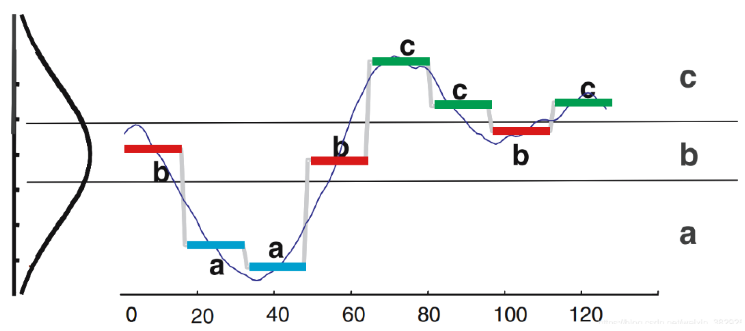
Among these, the SAX (Symbolic Aggregate Approximation) family of representation methods has received significant attention from researchers. As a data-adaptive representation method, SAX is known for its simplicity and comprehensibility. Its implementation mainly involves three steps: Z-normalizing the dataset, applying Piecewise Aggregate Approximation (PAA) for dimensionality reduction, and finally, performing symbolic representation. SAX has two important parameters: the dimensionality reduction parameter (w) and the alphabet size (α). Figure 1 illustrates the process of symbolization approximation for time series data of dimensionality 128. The original time series data are transformed into a string of length 8, represented as “baabccbc,” which contains three characters (a, b, c).
However, considering the complexity and diversity of time series data, using only the mean of time series data segments to represent their information may overlook some important features, resulting in limited expressive power of SAX. Therefore, several improved representation methods based on SAX have been proposed, such as SAX-TD [16] and SAX-BD [17]. These methods enhance the accuracy of similarity measurement by incorporating additional key feature information for each time series data subsegment during compression and dimensionality reduction.
The SAX-TD method represents the trend distance using the distance from the endpoint value to the mean, but it has limitations for sequences with complex variations. The SAX-BD method represents the trend distance using the distance from the maximum and minimum values to the mean, but it requires more symbol representations and has poor dimensionality reduction performance.
In this paper, we propose a new method called SAX-DM, where “DM” stands for Double Mean. To better quantify the trend of the subsegments, we further divide the segments obtained by the PAA algorithm into two parts. We use the distance from the mean of the left part to the overall mean as the symbol of trend distance, which intuitively represents the trend of the subsegments. However, considering the issue of positive and negative values, we represent the trend direction by the difference between the left mean and the time average. Since the PAA algorithm has already normalized the time series data, the range of the trend distance is Δq ∈ [−1, 1].
Compared to SAX-TD and SAX-BD, SAX-DM provides a better representation of the overall trend of time series data segments with complex variations. Additionally, SAX-DM only adds an extra character on top of SAX, requiring fewer symbols. In our experiments, we propose a novel similarity measurement method based on the SAX-DM representation. The experimental results demonstrate that SAX-DM outperforms SAX-BD and SAX-TD in terms of effectiveness. Furthermore, we prove that our novel distance measurement method guarantees a lower bound on the Euclidean distance while maintaining a more compact lower bound than the original SAX method.
2. Related Work
Assuming that time series data follow a normal distribution, according to mathematical principles, we can transform the original sequence data into a sequence that conforms to the standard normal distribution. The SAX representation method draws inspiration from this idea. It first segments the transformed sequence data and calculates the mean for each segment. Then, these means are mapped to corresponding probability intervals based on their magnitudes. If we assign a letter to each interval, we obtain a sequence of letters, which forms the basis of the SAX. Through this process, the SAX is able to transform the original continuous time series data into a discrete symbol sequence, thereby simplifying the representation and processing of the data.
2.1. Distance Calculation by SAX
The implementation of SAX mainly consists of three steps: Z-normalization of the dataset, dimensionality reduction using PAA, and finally symbolization. First of all, it is common to normalize the time series data so that each time series has a mean of 0 and a variance of 1 because time series data with different offsets and amplitudes are not directly comparable. Then, using a sliding-window approach, the original time series data are divided into w equal-length subsequences, and each subsequence is represented by its mean value. The normalized time series data follow a normal distribution, which provides mathematical support for dividing the probability distribution corresponding to the time series data into equal area regions and can ensure that the probability of the time series data falling into each interval is equal. The number of regions is determined by the input parameter α, which also represents the size of the character set. Each region is then represented by a symbol. Finally, based on the region in which the mean value of each subsequence falls, the corresponding symbol for that region is used to replace the subsequence, resulting in the symbolization approximation representation of the time series data.
Assuming we have two time series data Q and C with the same length n, which is divided into w time segments represented as q and c, and are the symbol strings obtained after applying the SAX algorithm. The SAX distance between Q and C can be calculated as the sum of the distance between each corresponding symbol and can be expressed as follows:
2.2. Two Improvements of SAX Distance Measure for Time Series
2.2.1. SAX-TD
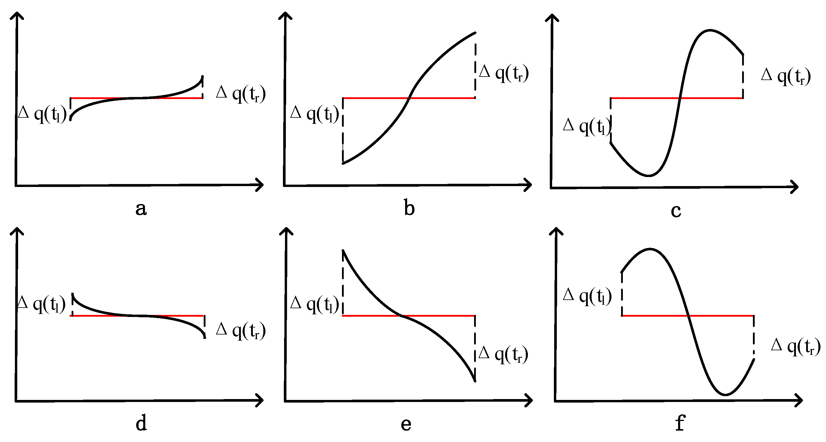
In order to enhance the accuracy of the SAX representation, it is important to preserve the trend information of the time series data during the dimensionality reduction process. For instance, the authors of reference [16] propose storing a value and a symbol in SAX to improve the distance calculation. They introduce an improvement method called SAX-TD, which utilizes the start and end points of segments to calculate the trend distance. There are several scenarios for the trend variation of time series data segments, as illustrated in Figure 2. In this figure, tl represents the left endpoint, which is the starting endpoint, and tr represents the right endpoint, which is the end endpoint.
The trend is indeed an important feature of time series data and plays a crucial role in their classification and analysis. For instance, if the endpoint value is greater than the starting point value, it indicates an upward trend, while the opposite suggests a downward trend. To describe this trend more accurately, it is necessary to use the actual values instead of the symbolized mapping when calculating the trend distance.
For the given time series data q and c, their trend distance is calculated as follows:
where and represents the left and right endpoint values of the time series segment, ∆q(t) represents the distance from the endpoint value to the average value of the line segment in the sequence, and q(∆c(t) represents the corresponding distance of another sequence), calculated using Formula (3):
Although each segment has a starting point and an endpoint, in practice, the starting point of the next segment is actually the endpoint of the previous segment. Therefore, it is possible to embed the trend distance into the SAX symbolized sequence. As a result, the time series data Q and C can be expressed using the following representation:
represents a sequence symbolized by SAX, and Δq(1), Δq(2), …, Δq(x) represents the trend of the time series data represented by the distance between the endpoint values and the mean values. Δq(x + 1) represents the change in the last point.
The distance measure formula for the time series data Q and C can be expressed as follows:
where represents the distance calculated using the SAX distance measure algorithm, represents the distance calculated using Equation (2), n represents the length of q and c, and w represents the number of time segments.
2.2.2. SAX-BD
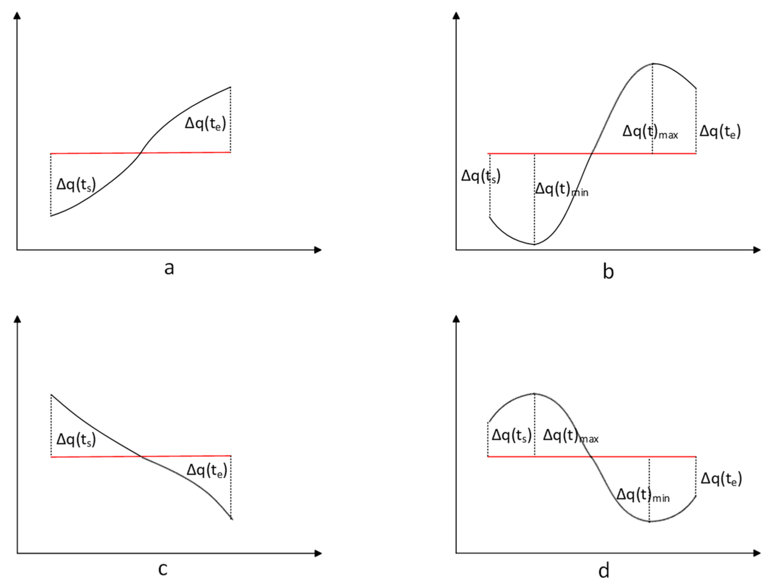
Reference [17] and others suggest adding boundary distance as a new consideration instead of trend distance and propose the algorithm SAX-BD. This algorithm considers that, for each segmented time series fragment, there are maximum and minimum points, and their distances to the mean value are referred to as the boundary distance. The average of the segment’s boundary distances contributes to a more accurate measurement of the different trends in the time series data. Details are provided below.
From Figure 3, we can observe that the maximum and minimum values within each time segment serve as the boundaries. The boundary distance of a is denoted as and , as shown in Equations (5) and (6):
In fact, the SAX-BD algorithm computes the trend changes (i.e., the boundary distance) of a as and , and these values are equivalent to and . Therefore, it is evident that SAX-BD can also effectively distinguish between them. For cases a and b, the distance calculated using SAX-TD is 0. However, in the SAX-BD approach, the distance calculated using SAX-BD is not equal to 0, indicating the potential for differentiation between these two sequences. Regarding the situations c and d, according to the TD and BD methods, it is as follows:
- for case c,
- for case d,
Similar to the SAX-TD distance measurement concept, the following SAX-BD distance measurement formula can be used for temporal data Q and C:
3. Our Method, SAX-DM
3.1. SAX-DM Design and Analysis
In the SAX algorithm, expressing the information of a time series segment solely based on its mean would overlook some important features, resulting in limited expressive power. The SAX-TD method represents trend distance using the distance from the endpoints to the mean, which has certain limitations for sequences with complex variations. The SAX-BD method represents trend distance using the distance from the maximum and minimum values to the mean, requiring more symbols for representation and resulting in poor dimensionality reduction.
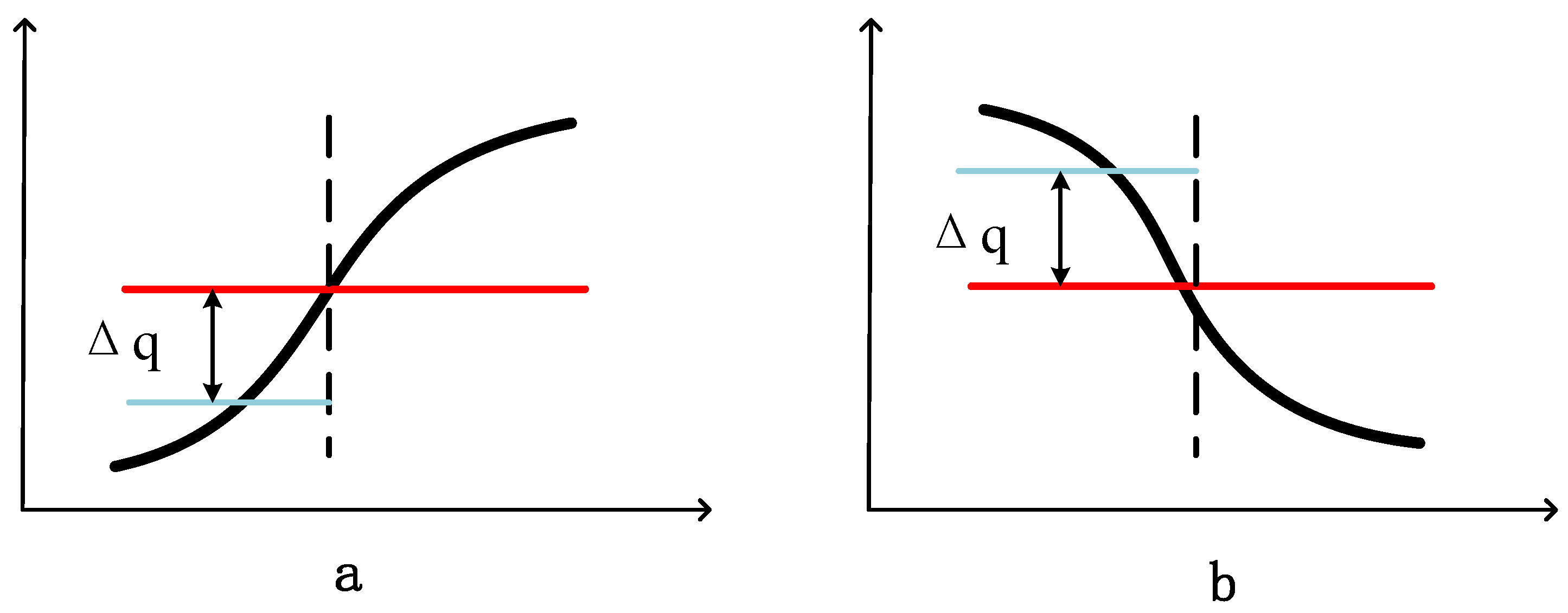
In this paper, we propose a new approach that utilizes the mean and trend of time series subsegments as key information. To better quantify the trend of the subsegments, we further divide the segments obtained through the PAA algorithm into two parts. The distance from the mean of the left part to the overall mean is used as the trend distance, which intuitively represents the trend of the subsegment. However, considering the issue of positive and negative values, we use the difference between the left mean and the time average mean to represent the trend. Since the PAA algorithm already normalizes the time series data, the trend distance range is Δq ∈ [−1, 1]. Figure 4 illustrates some examples of determining the trend distance. When the left mean in the segment is smaller than the overall mean, the trend is considered increasing, and the trend distance is positive, as shown in example in Figure 4a. When the left mean in the segment is larger than the overall mean, the trend is considered decreasing, and the trend distance is negative, as shown in example in Figure 4b.
Compared to SAX-TD and SAX-BD, SAX-DM can better represent the overall trend of time series data segments with complex variations, while requiring fewer symbols. For a segment with the mean value , its trend distance Δq can be represented within the range [−1, 1]. Therefore, when dividing time series data into n parts, it can be expressed as follows:
3.2. Similarity Measurement Based on SAX-DM Expression Method
In this paper, the Euclidean distance is employed as the fundamental method for measuring similarity. For a sequence approximated using SAX-DM, it can be viewed as a point in a w-dimensional space. Therefore, the computation of similarity between time series data can be transformed into calculating the distance between different points in this w-dimensional space.
Before proceeding, let us review the method for calculating Euclidean distance on the original time series data. Suppose we have two time series data, , . The Euclidean distance between them is the straight-line distance between the points represented by the two time series data objects in an n-dimensional space. It can be calculated using the following formula:
Due to the high-dimensional nature of time series data, calculating distances on the original time series data can lead to significant memory pressure and a substantial number of computations. This process is also susceptible to noise and deformations in the data. Therefore, it is common to compress and reduce the dimensionality of the original time series data and extract features. One popular method for compression and dimensionality reduction is using Piecewise Aggregate Approximation (PAA). After applying PAA, the similarity distance can be calculated using the following formula:
Each time series data subsegment uses the mean as a feature information:
In this article, trend distance is used to represent temporal data fragments. Firstly, a representation based on trend distance is defined. For temporal data Q and C, the following expressions are defined:
According to the above expression, the formula for calculating the trend distance based on the left mean value is defined as follows:
The distance measurement can be represented by the following equation:
In order to address the memory pressure and computational efficiency issues associated with high-dimensional time series data, it is generally necessary to compress and reduce the dimensionality of the original data and extract features. In this paper, the PAA method is employed to segment the original time series data, and the average value and change trend of subsegments are used as the key information for each subsegment. This approach aims to improve the compression ratio of the approximate representation while preserving the essential features of the original data as much as possible. Furthermore, by considering the trend of temporal data changes, the similarity measurement method based on the approximate representation proposed in this paper can calculate similarity more accurately.
3.3. Lower Bound
The SAX algorithm, when applied for dimensionality reduction, offers one of its most important features, that is providing a lower-bound distance measurement called the boundary distance. The lower bound is useful to control errors and accelerate computations. However, when performing spatial queries on the dimensionally reduced original sequence, there is a risk of false negatives. To reduce the occurrence of false negatives after dimensionality reduction, it is important to design algorithms that satisfy a good lower-bound property.
Next, we will prove that the distance we propose also serves as a lower bound for the Euclidean distance.
The lower bound of the PAA distance for the Euclidean distance is given by the following expression:
To prove that DMIST is also a lower bound for the Euclidean distance, we reiterate some of the proofs here. Let Q and C be the means of the time series data Q and C, respectively. Firstly, we consider the single-frame case (i.e., w = 1), and according to Equation (15), we can obtain
Recall that q is the average value of the temporal data, so can use . This also applies to each point c in . Equation (15) can be rewritten as follows:
Because and , we can obtain the following inequality (which clearly exists in the boundary distance ):
Substituting Equation (16) into Equation (17), we obtain
MINDIST conducted a lower-bound analysis of the PAA distance, namely,
In Equation (20), and are, respectively, the symbolic representations of Q and C in the original SAX. By transitivity, the following inequality is correct:
Recalling Equation (15), this means
N frames can be obtained by applying a single-frame proof on each frame, namely,
The quality of the lower boundary distances is usually measured by the compactness of the lower boundaries (TLB):
The value of TLB is within the range [0, 1]. The higher the TLB value, the better the quality. Recalling the distance metric in the equation, we can obtain that , which means that SAX-DM has a tighter lower bound than the original SAX distance.
4. Experimental Validation
In this section, we compare the classification results of SAX-DM representation with other representations on time series data through experiments. Firstly, we introduce the experimental dataset, followed by an explanation of the experimental methodology and parameter settings. Finally, we evaluate the advantages of SAX-DM based on the comprehensive assessment of classification accuracy and error rate.
4.1. Datasets
The evaluation of SAX-DM’s classification performance utilized the UCR Time Series Archive [28], which is a widely used collection of time series datasets in the field of time series data mining. This dataset was introduced in 2002 and has been continuously expanded over time. Due to its inclusion of time series datasets from various domains, it has become an important resource in the time series data mining community and is recommended by researchers working with time series data.
Initially, the dataset contained only 16 datasets. However, since its introduction in 2002, it has been expanded, and it currently includes 128 datasets. These datasets cover seven different domains: Device, ECG, Image, Motion, Sensor, Simulated, and Spectro. After careful analysis and verification of the data, it was found that some datasets had missing values, with some missing data lengths exceeding half of their original data lengths. As the similarity measurement method based on the approximate expression in this paper relies on the concept of Euclidean distance and is applicable to equally sized time series data, it cannot calculate the similarity between time series data of unequal lengths. Therefore, some datasets were excluded from the analysis. In the end, this paper selected 100 datasets from the UCR Time Series Archive, covering the aforementioned seven domains, for the purpose of conducting time series data classification experiments. The list of datasets used can be found in Table 2.
4.2. Experimental Methods and Parameter Settings
Since the SAX-DM, SAX, SAX-TD, and SAX-BD methods are all based on PAA for segmenting time series data, they involve the parameter window size, denoted as “w.” Additionally, the SAX, SAX-TD, and SAX-BD methods also involve the parameter symbol table size, denoted as “alpha.” For each dataset, we defined a set of parameter settings according to the specifications shown in Table 3. The range for the parameter “w” was set from 5 to 20, and the range for the parameter “alpha” was set from 3 to 16. For each dataset, we compared the classification accuracy obtained with different parameter settings and retained the best result for comparison. Furthermore, under the condition of achieving the best classification accuracy for each method, we compared the length ratio of the original sequence to the corresponding sequence obtained by different methods.
4.3. Experimental Results and Analysis
We compared the classification accuracy and error rate of SAX-DM with those of ED, SAX, SAX-TD, and SAX-BD. The experimental results show that in most of the datasets, SAX-DM achieved comparable accuracy to SAX-TD and SAX-BD, with the additional advantage of lower classification error rates.
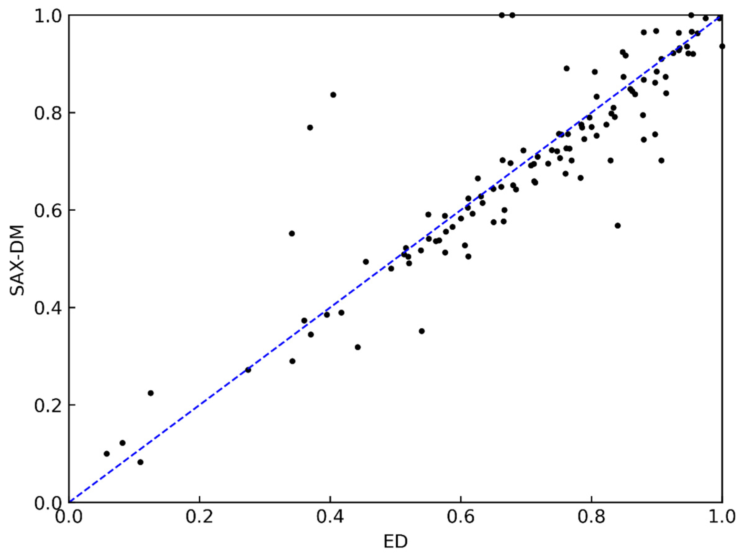
Figure 5 presents the comparison results between the SAX-DM and ED methods. Each point in the graph represents a dataset, where the x-axis represents the classification accuracy using the ED method, and the y-axis represents the classification accuracy using the SAX-DM method. Intuitively, the more points above the diagonal line, the more datasets in which the SAX-DM achieved higher accuracy compared to the ED method. After statistical analysis, it was found that SAX-DM had a slightly lower classification accuracy than ED in 67% of the datasets. This is because the Euclidean distance, which directly measures similarity on the original time series data without compression and dimension reduction, achieves high accuracy but puts a significant burden on computer memory and has lower computational efficiency. It is typically used as a comparative method to assess the viability of an approach and is not directly used for data mining tasks. Subsequent experiments on the data compression ratio did not require a comparison with the ED method. Although the SAX-DM may perform worse or on par with the Euclidean distance method in most datasets, the accuracy gap is within 0.1 for 80% of the datasets, indicating that it achieves effective data dimension reduction while maintaining a reasonably close accuracy level compared to the Euclidean distance method.
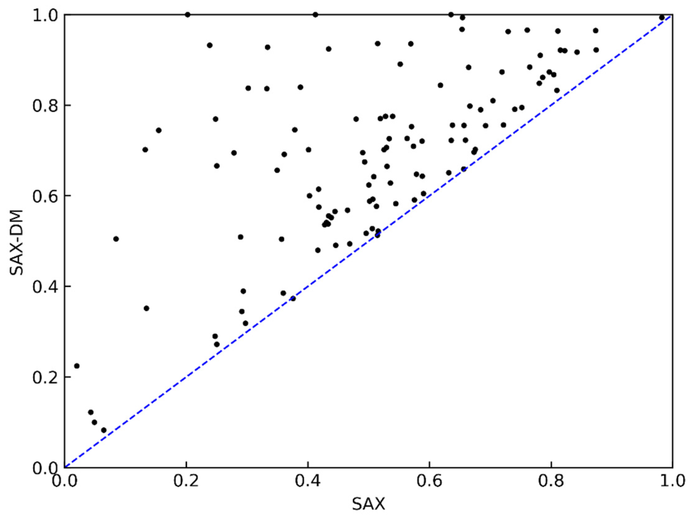
The comparison results between the SAX-DM and SAX methods in terms of classification accuracy are shown in Figure 6. The x-axis represents the classification accuracy using the SAX method, while the y-axis represents the classification accuracy using the SAX-DM method. The results represent the average classification accuracy for both representation methods under all α and w parameters, reflecting the overall classification performance. The results are evident, as using the SAX-DM method for approximate representation and similarity measurement in classification tasks yielded a higher accuracy in 98% of the datasets.
Compared to SAX, the SAX-DM further incorporates trend distance expression, allowing for better representation of the trend characteristics in time series data. However, this comes at the cost of sacrificing some data compression and dimension reduction rates. In practical usage, different methods can be chosen based on the application’s requirements for similarity accuracy in queries.
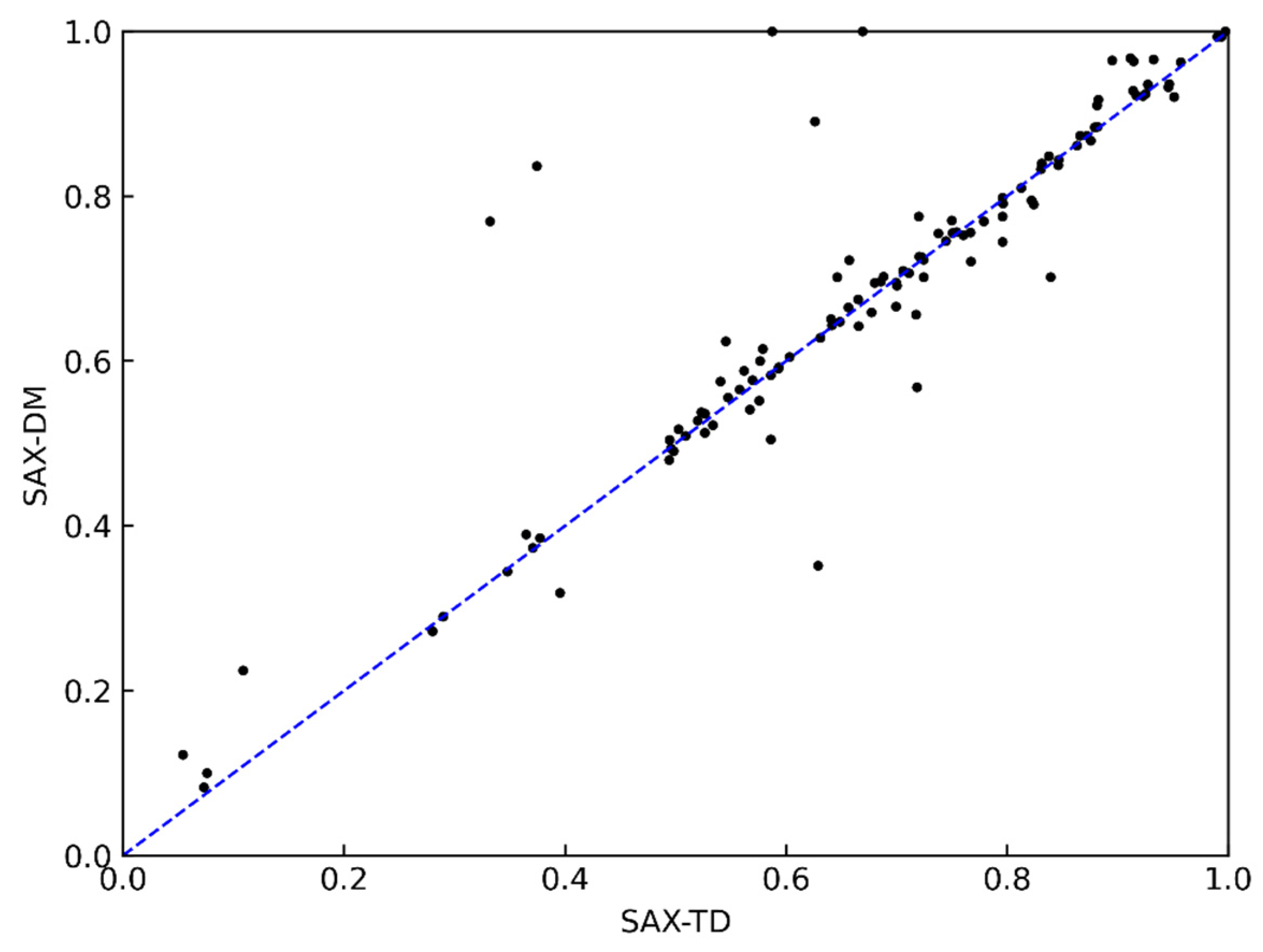
Figure 7 presents the comparison results between the SAX-DM and SAX-TD representation methods. From the figure, it can be observed that the two methods achieved similar accuracy in the classification task. When considering the reasons behind this, SAX-TD introduces a representation approach for capturing the trend by measuring the distance between the left and right endpoint values and the overall mean of the time series data. It combines this trend information with the mean value for symbolization. This approach is almost identical to the feature extraction methodology used in this paper, but it has certain limitations in practical applications. As the right endpoint value of one segment in time series data can be used as the left endpoint value of the next segment, when the number of segments is large, it is possible to approximate two symbols representing one segment. However, when the time series data have a small number of segments, the number of symbols required for the approximation representation increases.
In contrast, the SAX-DM method proposed in this paper can represent any segment of the time series data with two symbols, while still achieving a comparable classification accuracy to SAX-TD. Therefore, the SAX-DM method is more suitable for subsequent similarity query tasks on massive time series data. Additionally, the mean and trend distance can be further encoded to enhance compression and dimensionality reduction, thereby improving the compression ratio of the time series data approximation method.
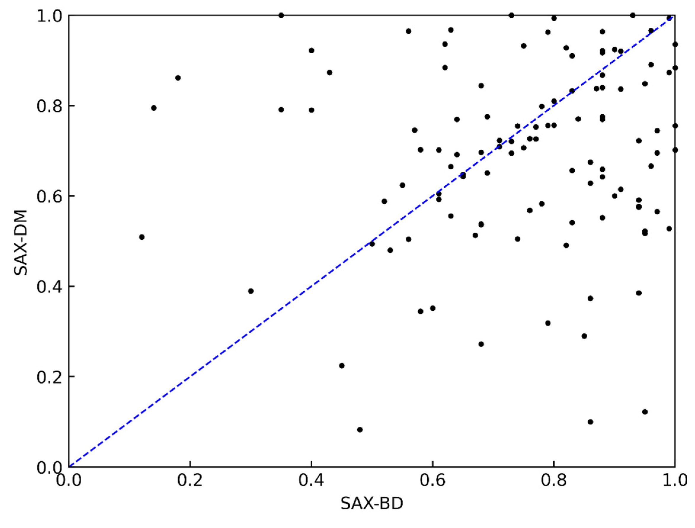
The comparison results between the SAX-DM and SAX-BD methods are shown in Figure 8. From the figure, it can be observed that the SAX-BD method performed better in the classification task on 60% of the datasets, and its classification accuracy varied significantly across different datasets. Considering the reasons behind this, the SAX-BD method incorporates the left and right extreme values in addition to the mean value to represent the time series data, while the SAX-DM method focuses on extracting the mean feature. Therefore, there is a significant difference in the expression effect of these two methods for data with smooth or drastic changes. Although SAX-BD achieves higher classification accuracy, it uses three features for dimensionality reduction, resulting in a lower compression ratio, which makes it unsuitable for subsequent similarity query tasks on large-scale time series data.
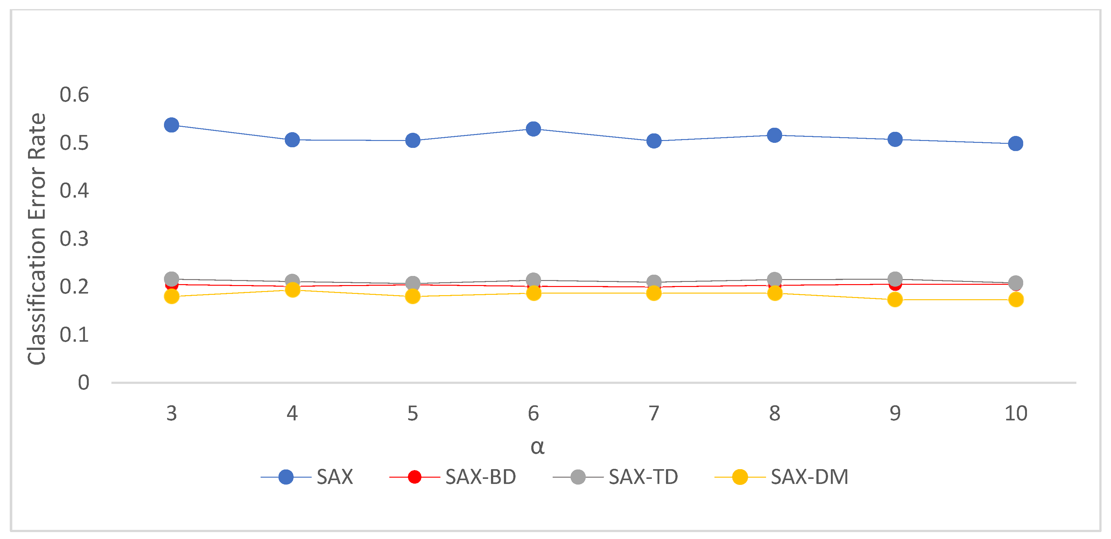
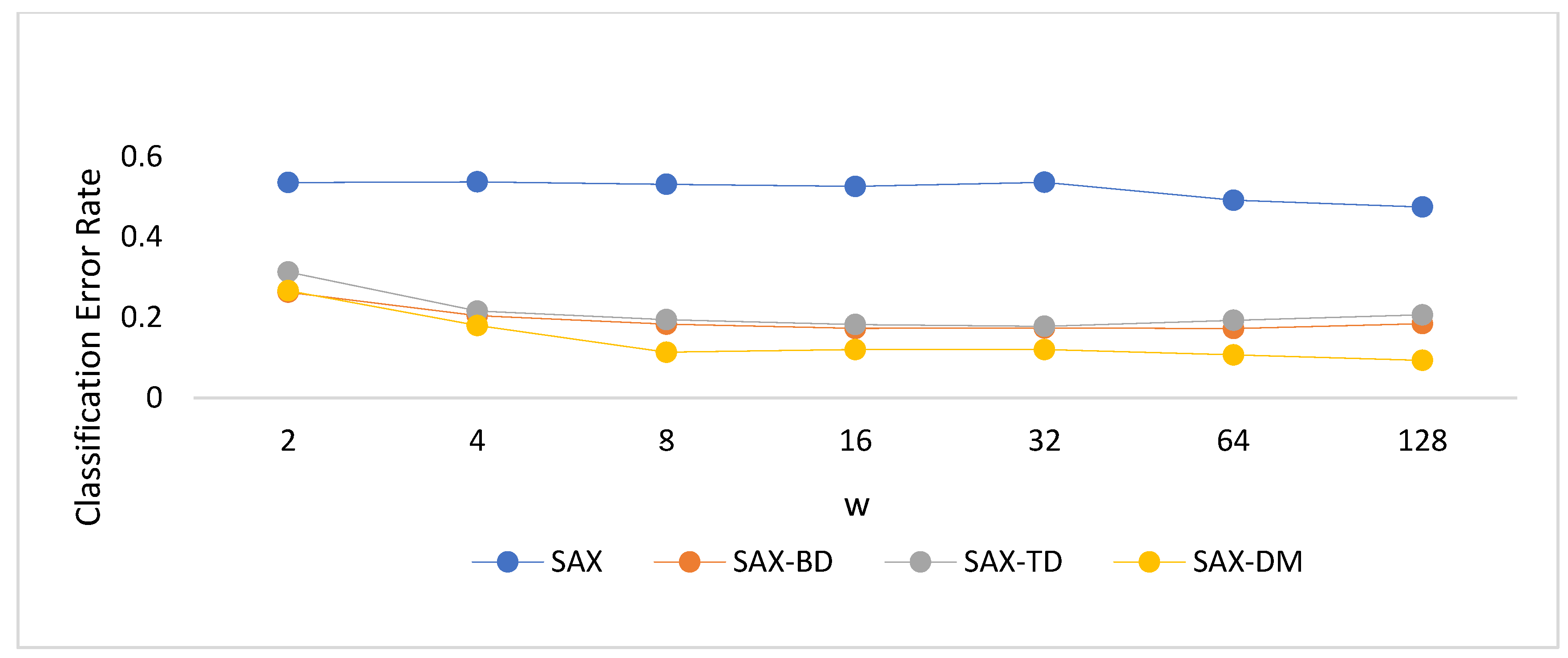
Figure 9 illustrates the comparison of classification error rates among the SAX, SAX-TD, SAX-BD, and SAX-DM methods using the classic ECG dataset as experimental data. Different α and w parameters were set for the evaluation. From the graph, it can be observed that the α parameter had a negligible impact on the classification accuracy, while the w parameter, when too large or too small, affected the accuracy. Based on the results depicted in the graph, the optimal value for the w parameter can be chosen as 16.
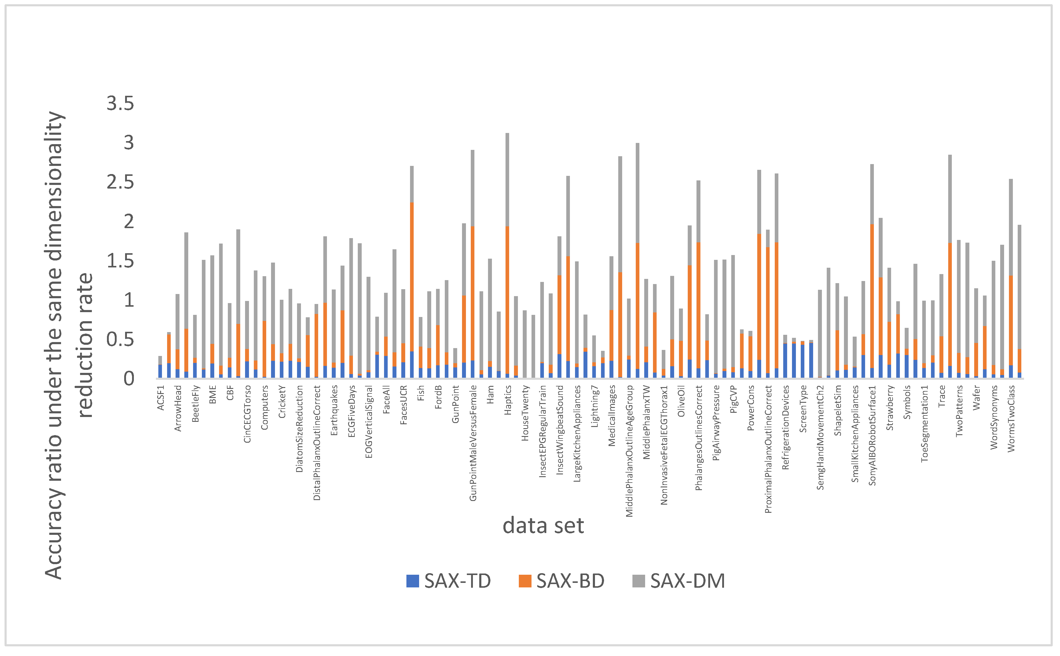
Since comparing compression ratios alone cannot fully demonstrate the advantages of expression methods, Figure 10 compares the classification accuracy of SAX, SAX-TD, SAX-BD, and SAX-DM at the same compression ratio, using SAX’s compression ratio as the benchmark. A higher value in the graph indicates better overall performance in terms of compression ratio and accuracy. It is evident from the graph that SAX-DM method performed exceptionally well and had a more convenient index item conversion method. In general, the SAX-DM method is more suitable for similarity queries in time series data, especially in scenarios that require a large number of iterations, as it effectively reduces computer memory pressure and enhances data mining efficiency.
5. Conclusions
The SAX-DM algorithm is proposed in this paper, taking into account the strengths and limitations of SAX-TD and SAX-BD. SAX-TD has limitations in handling complex sequences with varying patterns, while SAX-BD requires more symbols for representation. Our novel representation method adds an additional character to the original SAX, allowing for an intuitive representation of the change trend in subsegments. SAX-DM not only uses fewer characters to represent time series but also employs a new boundary distance measure to quantify time series similarity. Furthermore, we demonstrate that our distance measure maintains a lower bound on the Euclidean distance. Using this distance measure significantly reduces classification error rate, improves efficiency, and enhances accuracy in similarity calculations.
Author Contributions
Conceptualization, Z.H.; Methodology, Z.H. and C.Z.; Software, C.Z.; validation, Z.H., C.Z. and Y.C.; formal analysis, Y.C.; investigation, Y.C.; data curation, Y.C.; writing—original draft preparation, C.Z.; Writing—review & editing, Z.H. and C.Z.; visualization, Y.C.; supervision, Z.H.; Project administration, Z.H.; funding acquisition, Z.H. All authors have read and agreed to the published version of the manuscript.
Funding
This research was funded by the National Key Research and Development Program of China (2022YFF0801200,2022YFF0801203) and the National Natural Science Foundation of China (41972306).
Data Availability Statement
The data used in this experiment can be accessed through the URL https://www.cs.ucr.edu/~eamonn/time_series_data_2018/, accessed on 10 June 2023.
Acknowledgments
The work described in this paper was supported by the National Key Research and Development Program of China (2022YFF0801200,2022YFF0801203) and the National Natural Science Foundation of China (41972306). Thanks for the reviewers’ constructive comments; they really help us improve this paper.
Conflicts of Interest
The authors declare no conflict of interest.
References
- He, Z.; Wu, C.; Liu, G.; Tian, Y.; Zhang, X.; Chen, Q. Overview of similarity measurement and indexing methods for geoscience time series Big data. Bull. Geol. Sci. Technol. 2020, 39, 44–50. [Google Scholar]
- Agrawal, R.; Faloutsos, C.; Swami, A. Efficient similarity search in sequence databases. In Proceedings of the Foundations of Data Organization and Algorithms: 4th International Conference, FODO’93, Chicago, IL, USA, 13–15 October 1993; Springer: Berlin/Heidelberg, Germany, 1993; pp. 69–84. [Google Scholar]
- Chan, K.P.; Fu AW, C. Efficient time series matching by wavelets. In Proceedings of the 15th International Conference on Data Engineering (Cat. No. 99CB36337), Sydney, Australia, 23–26 March 1999; pp. 126–133. [Google Scholar]
- Korn, F.; Jagadish, H.V.; Faloutsos, C. Efficiently supporting ad hoc queries in large datasets of time sequences. SIGMOD Rec. 1997, 26, 289–300. [Google Scholar] [CrossRef]
- Yi, B.K.; Faloutsost, C. Fast Time Sequence Indexing for Arbitrary Lp Norms. 2000, pp. 385–394. Available online: https://www.vldb.org/conf/2000/P385.pdf (accessed on 10 February 2023).
- Fu, T.C.; Chung, F.L.; Luk, R.; Ng, C.-M. Representing financial time series based on data point importance. Eng. Appl. Artif. Intell. 2008, 21, 277–300. [Google Scholar] [CrossRef]
- Cai, Y.; Ng, R.T. Indexing Spatio-Temporal Trajectories with Chebyshev Polynomials. In Proceedings of the 2004 ACM SIGMOD International Conference on Management of Data, Paris, France, 13–18 June 2004; pp. 599–610. [Google Scholar]
- Chen, Q.; Chen, L.; Lian, X.; Liu, Y.; Yu, X. Indexable PLA for Efficient Similarity Search. In Proceedings of the 33rd International Conference on Very Large Data Bases, Vienna, Austria, 23–27 September 2007; pp. 435–446. [Google Scholar]
- Stefan, A.; Athitsos, V.; Das, G. The Move-Split-Merge Metric for Time Series. IEEE Trans. Knowl. Data Eng. 2013, 25, 1425–1438. [Google Scholar] [CrossRef] [Green Version]
- Zhang, Z.; Tang, P.; Duan, R. Dynamic time warping under pointwise shape context. Inf. Sci. 2015, 315, 88–101. [Google Scholar] [CrossRef]
- Keogh, E.J.; Pazzani, M.J. An enhanced representation of time series which allows fast and accurate classification, clustering and relevance feedback. InKdd 1998, 98, 239–243. [Google Scholar]
- Keogh, E.J. A Simple Dimensionality Reduction Technique for Fast Similarity Search in Large Time Series Databases. 2000, pp. 122–133. Available online: http://www.cs.ucr.edu/~eamonn/pakdd200_keogh.pdf (accessed on 16 February 2023).
- Chakrabarti, K.; Mehrotra, S.; Pazzani, M.; Keogh, E. Locally Adaptive Dimensionality Reduction for Indexing Large Time Series Databases. ACM Trans. Database Syst. 2002, 27, 188–228. [Google Scholar] [CrossRef] [Green Version]
- Lin, J.; Keogh, E.J.; Lonardi, S.; Chiu, B. A symbolic representation of time series, with implications for streaming algorithms. In Proceedings of the 8th ACM SIGMOD Workshop on Research Issues in Data Mining and Knowledge Discovery, San Diego, CA, USA, 13 June 2003; pp. 2–11. [Google Scholar]
- Lin, J.; Keogh, E.; Wei, L.; Lonardi, S. Experiencing SAX: A novel symbolic representation of time series. Data Min. Knowl. Discov. 2007, 15, 107–144. [Google Scholar] [CrossRef] [Green Version]
- Sun, Y.; Li, J.; Liu, J.; Sun, B.; Chow, C. An improvement of symbolic aggregate approximation distance measure for time series. Neurocomputing 2014, 138, 189–198. [Google Scholar] [CrossRef]
- He, Z.; Long, S.; Ma, X.; Zhao, H. A Boundary Distance-Based Symbolic Aggregate Approximation Method for Time Series Data. Algorithms 2020, 13, 284. [Google Scholar] [CrossRef]
- He, Z.; Zhang, C.; Ma, X.; Liu, G. Hexadecimal Aggregate Approximation Representation and Classification of Time Series Data. Algorithms 2021, 14, 353. [Google Scholar] [CrossRef]
- Yang, D.; Kang, Y. Distance- and Momentum-Based Symbolic Aggregate Approximation for Highly Imbalanced Classification. Sensors 2022, 22, 5095. [Google Scholar] [CrossRef] [PubMed]
- Huang, J.; Xu, X.; Cui, X.; Kang, J.; Yang, H. Time series data symbol aggregation approximation method for fusing trend information. Appl. Res. Comput. 2023, 40, 86–90. [Google Scholar]
- Ratanamahatana, C.; Keogh, E.; Bagnall, A.J.; Lonardi, S. A novel bit level time series representation with implication of similarity search and clustering. In Advances in Knowledge Discovery and Data Mining, Proceedings of the 9th Pacific-Asia Conference, PAKDD 2005, Hanoi, Vietnam, 18–20 May 2005; Springer: Berlin/Heidelberg, Germany, 2005; pp. 771–777. [Google Scholar]
- Baydogan, M.G.; Runger, G.C. Learning a symbolic representation for multivariate time series classification. Data Min. Knowl. Discov. 2015, 29, 400–422. [Google Scholar] [CrossRef]
- Azzouzi, M.; Nabney, I.T. Analysing time series structure with hidden Markov models. In Neural Networks for Signal Processing VIII, Proceedings of the 1998 IEEE Signal Processing Society Workshop (Cat. No. 98TH8378), Cambridge, UK, 31 August–3 September 1998; IEEE: Piscataway, NJ, USA, 1998; pp. 402–408. [Google Scholar]
- Serra, J.; Kantz, H.; Serra, X.; Andrzejak, R.G. Predictability of Music Descriptor Time Series and its Application to Cover Song Detection. IEEE Trans. Audio Speech Lang. Process. 2012, 20, 514–525. [Google Scholar] [CrossRef] [Green Version]
- Baydogan, M.G.; Runger, G.C. Time series representation and similarity based on local autopatterns. Data Min. Knowl. Discov. 2016, 30, 476–509. [Google Scholar] [CrossRef]
- Ye, Y.; Jiang, J.; Ge, B.; Dou, Y.; Yang, K. Similarity measures for time series data classification using grid representation and matrix distance. Knowl. Inf. Syst. 2019, 60, 1105–1134. [Google Scholar] [CrossRef]
- Su, Z.; Liu, Q.; Zhao, C.; Sun, F. A Traffic Event Detection Method Based on Random Forest and Permutation Importance. Mathematics 2022, 10, 873. [Google Scholar] [CrossRef]
- Dau, H.A.; Bagnall, A.; Kamgar, K.; Yeh, C.-C.M.; Zhu, Y.; Gharghabi, S.; Ratanamahatana, C.A.; Keogh, E. The UCR Time Series Archive. IEEE/CAA J. Autom. Sin. 2019, 6, 6–18. [Google Scholar] [CrossRef]
Figure 1.
Symbolized approximate representation of time series data SAX.

Figure 2.
Some examples of SAX-TD. (a–f) represent the trend distances calculated by the SAX-TD method for representing sequences of various common shapes.
Figure 2.
Some examples of SAX-TD. (a–f) represent the trend distances calculated by the SAX-TD method for representing sequences of various common shapes.

Figure 3.
Some cases of SAX-BD. (a–d) represent four sequences with the same size mean, where the left and right endpoints of (a,b) are the same, while the maximum and minimum values of (c,d) are the same, respectively.
Figure 3.
Some cases of SAX-BD. (a–d) represent four sequences with the same size mean, where the left and right endpoints of (a,b) are the same, while the maximum and minimum values of (c,d) are the same, respectively.

Figure 4.
Schematic diagram of SAX-DM trend distance. (a) represents the trend distance calculated by the SAX-DM method for sequences with an upward trend. (b) represents the trend distance calculated by the SAX-DM method for sequences with a downward trend.
Figure 4.
Schematic diagram of SAX-DM trend distance. (a) represents the trend distance calculated by the SAX-DM method for sequences with an upward trend. (b) represents the trend distance calculated by the SAX-DM method for sequences with a downward trend.

Figure 5.
Comparison results of SAX-DM and ED.

Figure 6.
Comparison results of SAX-DM and SAX.

Figure 7.
Comparison results of SAX-DM and SAX-TD.

Figure 8.
Comparison results of SAX-DM and SAX-BD.

Figure 9.
Comparison of classification error rates under different α and w conditions.


Figure 10.
SAX and its improved method accuracy and compression ratio.


Table 1.
Main representation methods of time series data.
| Representation | Publication Time | Type | Algorithm Complexity | Method Source |
|---|---|---|---|---|
| Discrete Fourier Transform (DFT) | 1993 | T1 | O(n(log(n))) | [2] |
| Discrete Wavelet Transform (DWT) | 1999 | T1 | O(n) | [3] |
| Discrete Cosine Transform (DCT) | 1997 | T1 | N | [4] |
| Partitioned Aggregation Approximation (PAA) | 2000 | T1 | O(n) | [5] |
| Perceived Importance Points (PIPs) | 2001 | T1 | N | [6] |
| Chebyshev Polynomials (CHEBs) | 2004 | T1 | N | [7] |
| Indexable Piecewise Linear Approximation (IPLA) | 2007 | T1 | N | [8] |
| Move Split Merge (MSM) | 2013 | T1 | N | [9] |
| Graphical-Content-Based DTW (SC DTW) | 2015 | T1 | N | [10] |
| Singular Value Decomposition (SVD) | 1997 | T2 | O(Mn2) | [4] |
| Piecewise Linear Approximation (PLA) | 1998 | T2 | O(n(log(n))) | [11] |
| Piecewise Constant Approximation (PCA) | 2000 | T2 | N | [12] |
| Adaptive Partitioning Constant Approximation (APCA) | 2002 | T2 | O(n) | [13] |
| Symbolized Aggregate Approximation (SAX) | 2003 | T2 | O(n) | [14,15] |
| SAX Based on Trend Distance (SAX-TD) | 2014 | T2 | N | [16] |
| SAX Based on Boundary Distance (SAX-BD) | 2020 | T2 | N | [17] |
| Hexadecimal Aggregate Approximation (HAX) | 2021 | T2 | N | [18] |
| Point Aggregation Approximation (PAX) | 2021 | T2 | N | [18] |
| Symbol Aggregation Approximation Based on Distance and Momentum | 2022 | T2 | N | [19] |
| Convergence Trend Symbol Aggregation Approximation (SAX-TI) | 2023 | T2 | N | [20] |
| Clipped Data | 2005 | T3 | N | [21] |
| Tree-Based Representation Method | 2015 | T3 | N | [22] |
| Hidden Markov Models (HMMs) | 1998 | T4 | N | [23] |
| Automatic Regression Model | 2012 | T4 | N | [24] |
| Representation Method Based on Local Automatic Mode | 2016 | T4 | N | [25] |
| Grid-Based Representation Method | 2019 | T4 | N | [26] |
| Based on Random Forest and Ranking Importance | 2022 | T4 | N | [27] |
N: author not listed. T1: non-data-adaptive representation methods. T2: data-adaptive representation methods. T3: data-indicative representation methods. T4: model-based representation methods.
Table 2.
List of time series datasets.
| Id | Type | Name | Train | Test | Class | Length |
|---|---|---|---|---|---|---|
| 1 | Device | ACSF1 | 100 | 100 | 10 | 1460 |
| 2 | Image | Adiac | 390 | 391 | 37 | 176 |
| 3 | Image | ArrowHead | 36 | 175 | 3 | 251 |
| 4 | Spectro | Beef | 30 | 30 | 5 | 470 |
| 5 | Image | BeetleFly | 20 | 20 | 2 | 512 |
| 6 | Image | BirdChicken | 20 | 20 | 2 | 512 |
| 7 | Simulated | BME | 30 | 150 | 3 | 128 |
| 8 | Sensor | Car | 60 | 60 | 4 | 577 |
| 9 | Simulated | CBF | 30 | 900 | 3 | 128 |
| 10 | Traffic | Chinatown | 20 | 343 | 2 | 24 |
| 11 | Sensor | CinCECGTorso | 40 | 1380 | 4 | 1639 |
| 12 | Spectro | Coffee | 28 | 28 | 2 | 286 |
| 13 | Device | Computers | 250 | 250 | 2 | 720 |
| 14 | Motion | CricketX | 390 | 390 | 12 | 300 |
| 15 | Motion | CricketY | 390 | 390 | 12 | 300 |
| 16 | Motion | CricketZ | 390 | 390 | 12 | 300 |
| 17 | Image | DiatomSizeReduction | 16 | 306 | 4 | 345 |
| 18 | Image | DistalPhalanxOutlineAgeGroup | 400 | 139 | 3 | 80 |
| 19 | Image | DistalPhalanxOutlineCorrect | 600 | 276 | 2 | 80 |
| 20 | Image | DistalPhalanxTW | 400 | 139 | 6 | 80 |
| 21 | Sensor | Earthquakes | 322 | 139 | 2 | 512 |
| 22 | ECG | ECG200 | 100 | 100 | 2 | 96 |
| 23 | ECG | ECGFiveDays | 23 | 861 | 2 | 136 |
| 24 | EOG | EOGHorizontalSignal | 362 | 362 | 12 | 1250 |
| 25 | EOG | EOGVerticalSignal | 362 | 362 | 12 | 1250 |
| 26 | Spectro | EthanolLevel | 504 | 500 | 4 | 1751 |
| 27 | Image | FaceAll | 560 | 1690 | 14 | 131 |
| 28 | Image | FaceFour | 24 | 88 | 4 | 350 |
| 29 | Image | FacesUCR | 200 | 2050 | 14 | 131 |
| 30 | Image | FiftyWords | 450 | 455 | 50 | 270 |
| 31 | Image | Fish | 175 | 175 | 7 | 463 |
| 32 | Sensor | FordA | 3601 | 1320 | 2 | 500 |
| 33 | Sensor | FordB | 3636 | 810 | 2 | 500 |
| 34 | HRM | Fungi | 18 | 186 | 18 | 201 |
| 35 | Motion | GunPoint | 50 | 150 | 2 | 150 |
| 36 | Motion | GunPointAgeSpan | 135 | 316 | 2 | 150 |
| 37 | Motion | GunPointMaleVersusFemale | 135 | 316 | 2 | 150 |
| 38 | Motion | GunPointOldVersusYoung | 136 | 315 | 2 | 150 |
| 39 | Spectro | Ham | 109 | 105 | 2 | 431 |
| 40 | Image | HandOutlines | 1000 | 370 | 2 | 2709 |
| 41 | Motion | Haptics | 155 | 308 | 5 | 1092 |
| 42 | Image | Herring | 64 | 64 | 2 | 512 |
| 43 | Device | HouseTwenty | 40 | 119 | 2 | 2000 |
| 44 | Motion | InlineSkate | 100 | 550 | 7 | 1882 |
| 45 | EPG | InsectEPGRegularTrain | 62 | 249 | 3 | 601 |
| 46 | EPG | InsectEPGSmallTrain | 17 | 249 | 3 | 601 |
| 47 | Sensor | InsectWingbeatSound | 220 | 1980 | 11 | 256 |
| 48 | Sensor | ItalyPowerDemand | 67 | 1029 | 2 | 24 |
| 49 | Device | LargeKitchenAppliances | 375 | 375 | 3 | 720 |
| 50 | Sensor | Lightning2 | 60 | 61 | 2 | 637 |
| 51 | Sensor | Lightning7 | 70 | 73 | 7 | 319 |
| 52 | Spectro | Meat | 60 | 60 | 3 | 448 |
| 53 | Image | MedicalImages | 381 | 760 | 10 | 99 |
| 54 | Traffic | MelbournePedestrian | 1194 | 2439 | 10 | 24 |
| 55 | Image | MiddlePhalanxOutlineAgeGroup | 400 | 154 | 3 | 80 |
| 56 | Image | MiddlePhalanxOutlineCorrect | 600 | 291 | 2 | 80 |
| 57 | Image | MiddlePhalanxTW | 399 | 154 | 6 | 80 |
| 58 | Sensor | MoteStrain | 20 | 1252 | 2 | 84 |
| 59 | ECG | NonInvasiveFetalECGThorax1 | 1800 | 1965 | 42 | 750 |
| 60 | ECG | NonInvasiveFetalECGThorax2 | 1800 | 1965 | 42 | 750 |
| 61 | Spectro | OliveOil | 30 | 30 | 4 | 570 |
| 62 | Image | OSULeaf | 200 | 242 | 6 | 427 |
| 63 | Image | PhalangesOutlinesCorrect | 1800 | 858 | 2 | 80 |
| 64 | Sensor | Phoneme | 214 | 189 | 39 | 1024 |
| 65 | Hemodynamics | PigAirwayPressure | 104 | 208 | 52 | 2000 |
| 66 | Hemodynamics | PigArtPressure | 104 | 208 | 52 | 2000 |
| 67 | Hemodynamics | PigCVP | 104 | 208 | 52 | 2000 |
| 68 | Sensor | Plane | 105 | 105 | 7 | 144 |
| 69 | Power | PowerCons | 180 | 180 | 2 | 144 |
| 70 | Image | ProximalPhalanxOutlineAgeGroup | 400 | 205 | 3 | 80 |
| 71 | Image | ProximalPhalanxOutlineCorrect | 600 | 291 | 2 | 80 |
| 72 | Image | ProximalPhalanxTW | 400 | 205 | 6 | 80 |
| 73 | Device | RefrigerationDevices | 375 | 375 | 3 | 720 |
| 74 | Spectrum | Rock | 20 | 50 | 4 | 2844 |
| 75 | Device | ScreenType | 375 | 375 | 3 | 720 |
| 76 | Spectrum | SemgHandGenderCh2 | 300 | 600 | 2 | 1500 |
| 77 | Spectrum | SemgHandMovementCh2 | 450 | 450 | 6 | 1500 |
| 78 | Spectrum | SemgHandSubjectCh2 | 450 | 450 | 5 | 1500 |
| 79 | Simulated | ShapeletSim | 20 | 180 | 2 | 500 |
| 80 | Image | ShapesAll | 600 | 600 | 60 | 512 |
| 81 | Device | SmallKitchenAppliances | 375 | 375 | 3 | 720 |
| 82 | Simulated | SmoothSubspace | 150 | 150 | 3 | 15 |
| 83 | Sensor | SonyAIBORobotSurface1 | 20 | 601 | 2 | 70 |
| 84 | Sensor | SonyAIBORobotSurface2 | 27 | 953 | 2 | 65 |
| 85 | Spectro | Strawberry | 613 | 370 | 2 | 235 |
| 86 | Image | SwedishLeaf | 500 | 625 | 15 | 128 |
| 87 | Image | Symbols | 25 | 995 | 6 | 398 |
| 88 | Simulated | SyntheticControl | 300 | 300 | 6 | 60 |
| 89 | Motion | ToeSegmentation1 | 40 | 228 | 2 | 277 |
| 90 | Motion | ToeSegmentation2 | 36 | 130 | 2 | 343 |
| 91 | Sensor | Trace | 100 | 100 | 4 | 275 |
| 92 | ECG | TwoLeadECG | 23 | 1139 | 2 | 82 |
| 93 | Simulated | TwoPatterns | 1000 | 4000 | 4 | 128 |
| 94 | Simulated | UDM | 36 | 144 | 3 | 150 |
| 95 | Sensor | Wafer | 1000 | 6164 | 2 | 152 |
| 96 | Spectro | Wine | 57 | 54 | 2 | 234 |
| 97 | Image | WordSynonyms | 267 | 638 | 25 | 270 |
| 98 | Motion | Worms | 181 | 77 | 5 | 900 |
| 99 | Motion | WormsTwoClass | 181 | 77 | 2 | 900 |
| 100 | Image | Yoga | 300 | 3000 | 2 | 426 |
Table 3.
Approximate expression method parameters.
| Method | Parameter |
|---|---|
| ED | null |
| SAX-DM | |
| SAX | |
| SAX-TD | |
| SAX-BD |
Disclaimer/Publisher’s Note: The statements, opinions and data contained in all publications are solely those of the individual author(s) and contributor(s) and not of MDPI and/or the editor(s). MDPI and/or the editor(s) disclaim responsibility for any injury to people or property resulting from any ideas, methods, instructions or products referred to in the content. |
© 2023 by the authors. Licensee MDPI, Basel, Switzerland. This article is an open access article distributed under the terms and conditions of the Creative Commons Attribution (CC BY) license (https://creativecommons.org/licenses/by/4.0/).
Share and Cite
MDPI and ACS Style
He, Z.; Zhang, C.; Cheng, Y. Similarity Measurement and Classification of Temporal Data Based on Double Mean Representation. Algorithms 2023, 16, 347. https://doi.org/10.3390/a16070347
AMA Style
He Z, Zhang C, Cheng Y. Similarity Measurement and Classification of Temporal Data Based on Double Mean Representation. Algorithms. 2023; 16(7):347. https://doi.org/10.3390/a16070347
Chicago/Turabian StyleHe, Zhenwen, Chi Zhang, and Yunhui Cheng. 2023. "Similarity Measurement and Classification of Temporal Data Based on Double Mean Representation" Algorithms 16, no. 7: 347. https://doi.org/10.3390/a16070347
Note that from the first issue of 2016, this journal uses article numbers instead of page numbers. See further details here.