
On a Hypothetical Model with Second Kind Chebyshev’s Polynomial–Correction: Type of Limit Cycles, Simulations, and Possible Applications

1
Faculty of Mathematics and Informatics, University of Plovdiv Paisii Hilendarski, 24, Tzar Asen Str., 4000 Plovdiv, Bulgaria
2
Institute of Mathematics and Informatics, Bulgarian Academy of Sciences, Acad. G. Bonchev Str., Bl. 8, 1113 Sofia, Bulgaria
*
Author to whom correspondence should be addressed.
†
These authors contributed equally to this work.
Algorithms 2022, 15(12), 462; https://doi.org/10.3390/a15120462
Submission received: 2 November 2022
/
Revised: 30 November 2022
/
Accepted: 30 November 2022
/
Published: 6 December 2022
(This article belongs to the Special Issue Computational Methods and Optimization for Numerical Analysis)
Abstract
:In this article, we explore a new extended Lienard-type planar system with “corrections” of the second kind Chebyshev’s polynomial . The number and type of limit cycles are also studied. The discussion on the —component of the solution of the Lienard system is connected to searching for the solution of the synthesis of filters and electrical circuits. Numerical experiments, depicting our outcomes using CAS MATHEMATICA, are presented.
1. Introduction
Hilbert [1] proposed 23 mathematical problems, of which the second part of the 16th one is to find the maximal number of limit cycles and their relative locations for polynomial vector fields. A large part of the scientific articles is concerned with the Lienard system , where is a small parameter and and are polynomials of degree m and n.
The Melnikov polynomial is defined as
Perko and collaborators [4,5] ensure the needful information about radii and the number of limit cycles. More precisely, the system (1) for small enough has at most nlimit cycles asymptotic to circles of radii as if and only if then-th degree polynomial in ,
has n positive roots .
Denote by the second kind Chebyshev’s polynomial. The polynomials participate in the solution to some of the practical tasks [6]. In this article, we explore a new extended Lienard-type planar system with the polynomial . The number and type of limit cycles is also investigated. The discussion (in Section 2.3) is on —the component of the solution of Lienard system that is connected to the solution of some practical issues such as the synthesis of “adaptive” filters and electrical circuits. Numerical examples, confirming the results we obtained through CAS MATHEMATICA, are received.
2. Main Results–Simulations
2.1. Extended Lienard-Type Planar System
The next model will be investigated:
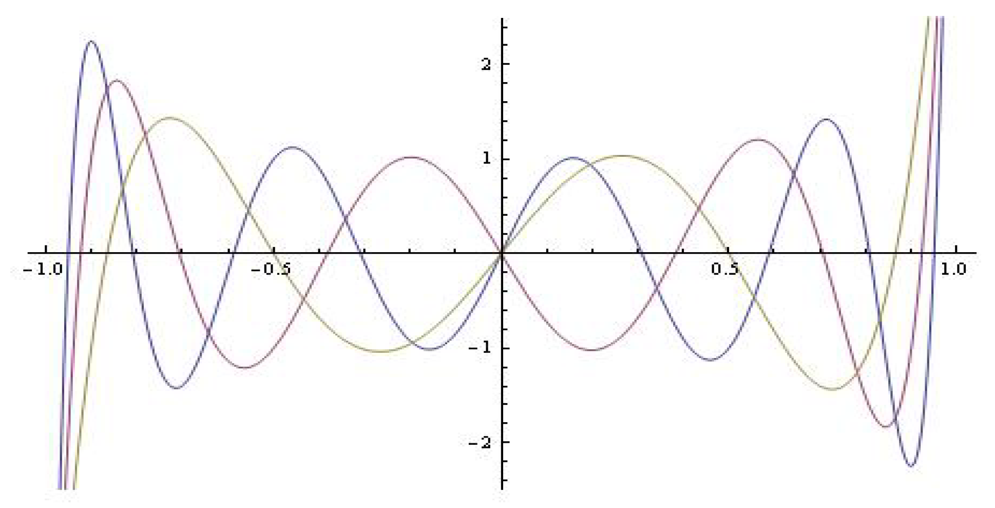
where and for is the Chebyshev’s polynomial of the second kind. For example, for we have (see Figure 1)
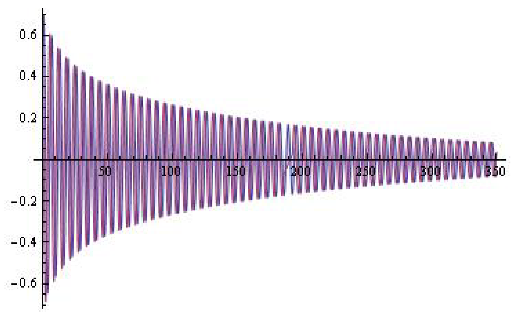
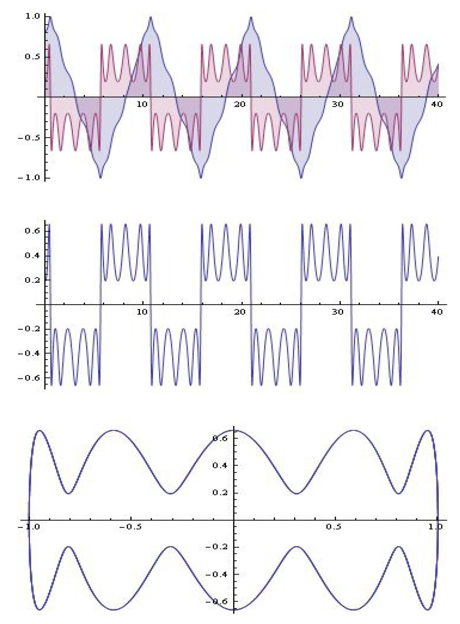
Under stated circumstances it can be indicated that the Lienard’s-type system (1) has a limit cycle. The proof of existence of the limit cycle is based on the check of the circumstances in Lienard’s theorem [3], and we will skip it. The process for user-initiated coefficient and , with the model (5) for , is shown in Figure 2. For and and , see Figure 3. The simulation for and , with the model (5) for , , is shown in Figure 4. For and ; , , see Figure 5.
2.2. The New Model in the Light of Melnikov’s Considerations
The case . Let us explore the model
where , . The following is correct:
Proposition 1.
The Lienard-type system (6) for , and for all small enough for has a limit cycle with multiplicity–2.
Proof.
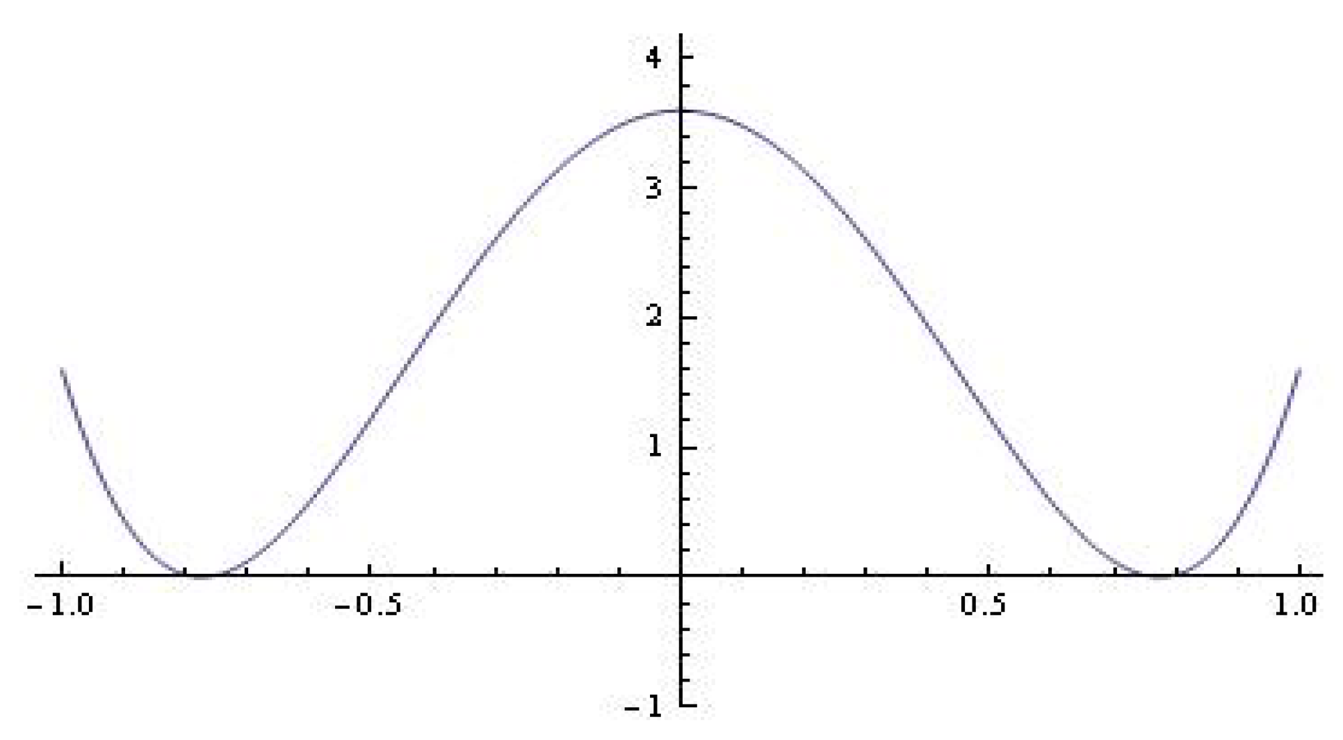
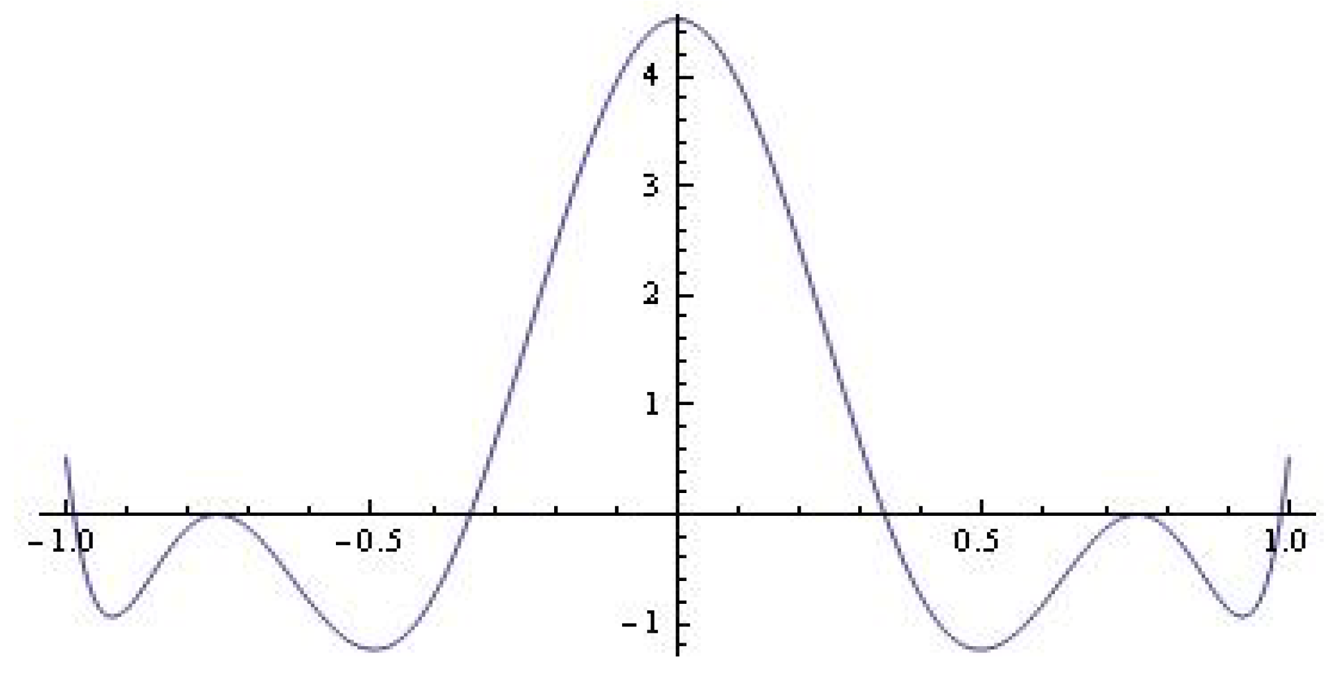
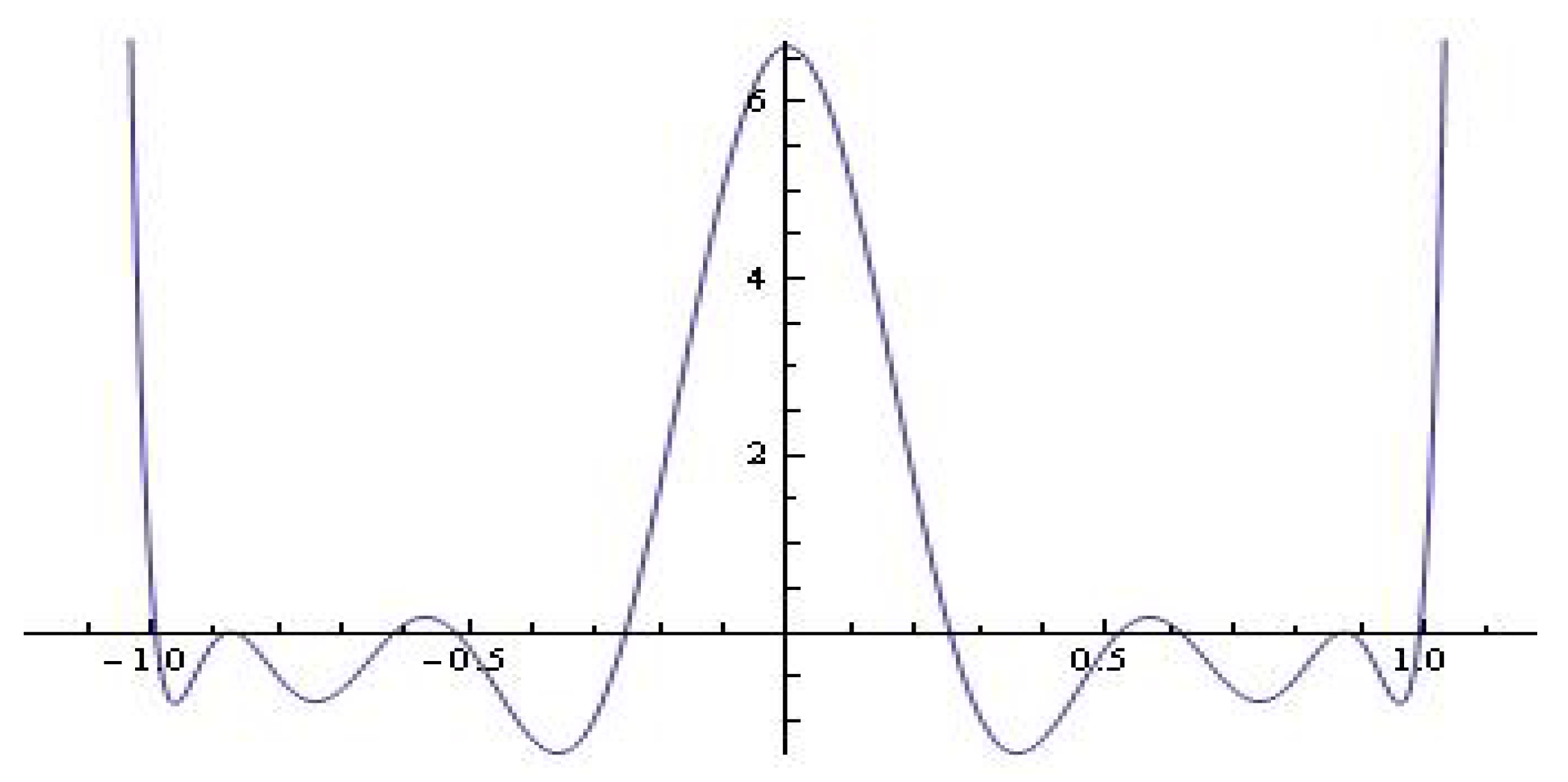
For the Melnikov polynomial in (see Figure 6), we have:
□
The roots are
The radii for some values of are tabulated in Table 1.
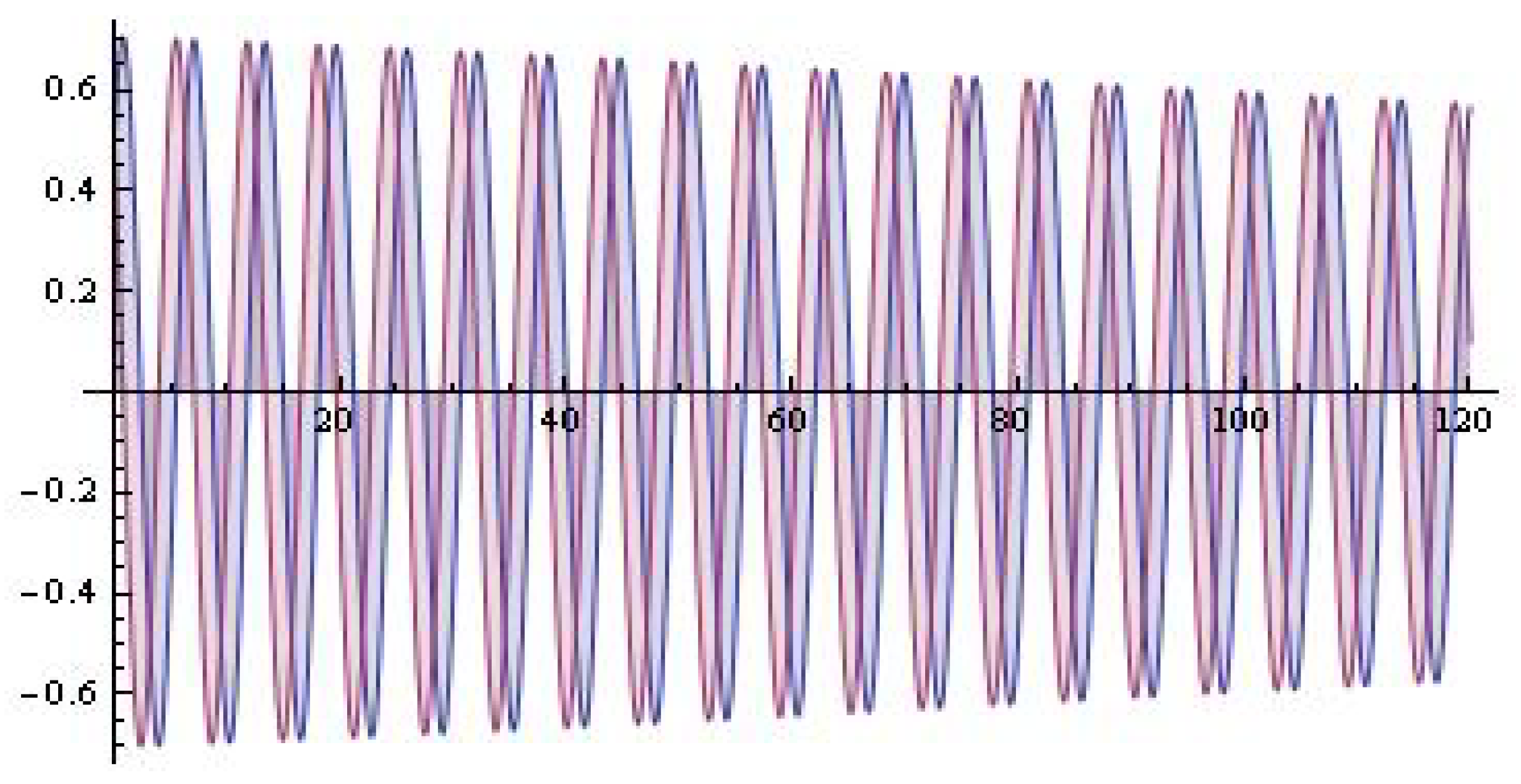
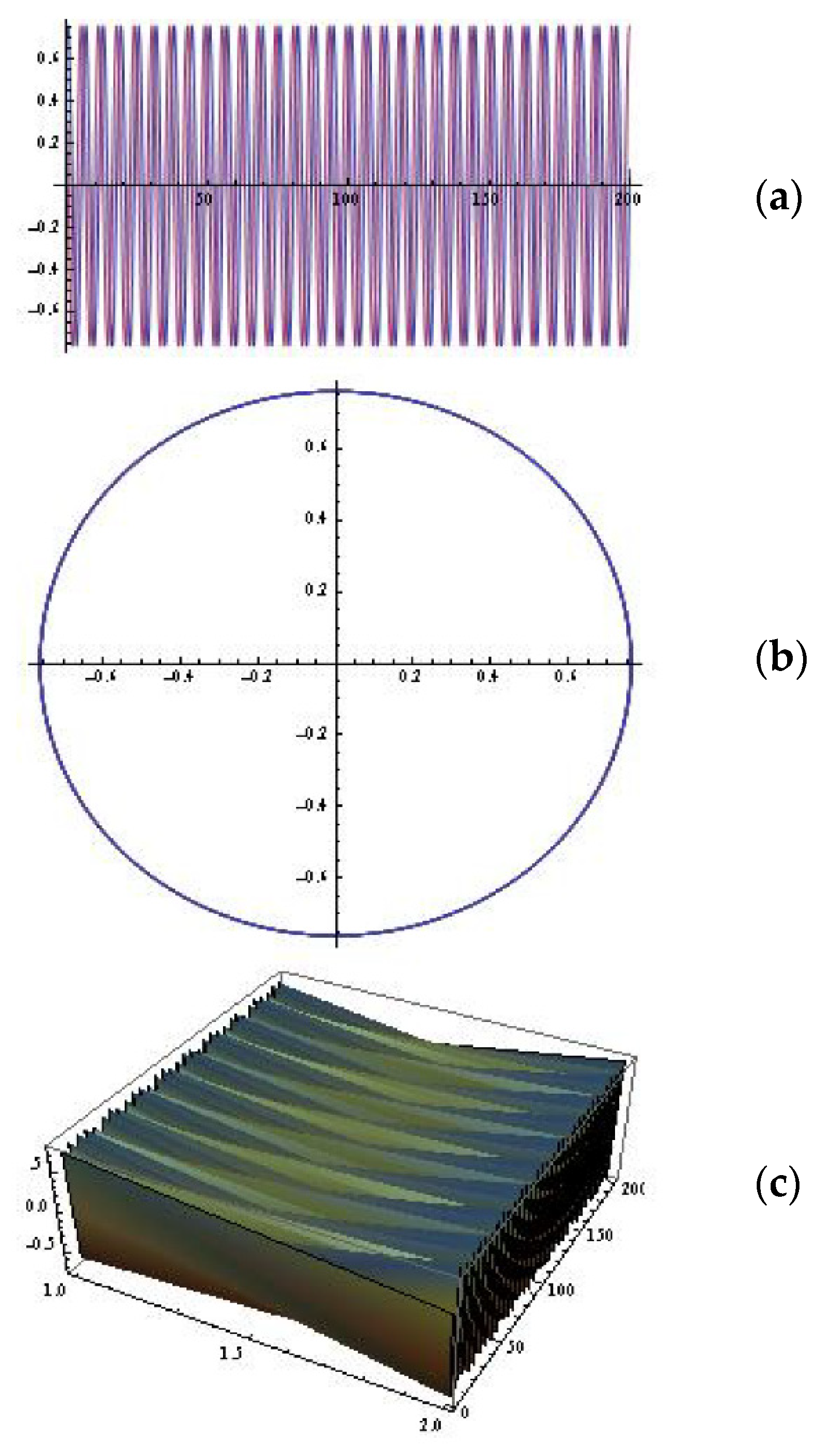
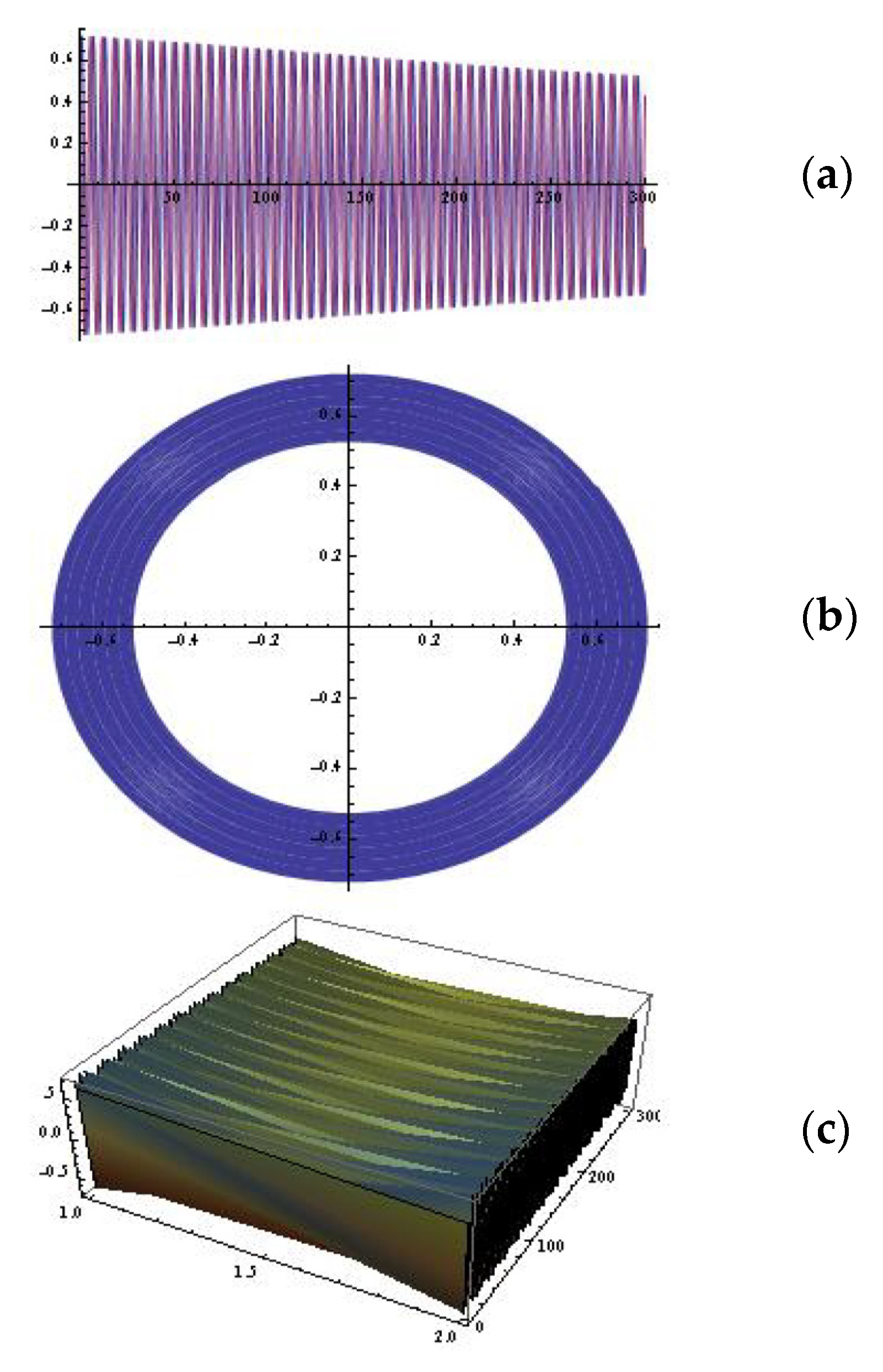
Evidently, for example we obtain a limit cycle with multiplicity–2 (see Table 1). This ends the proof of the proposition. The solution of the system (6) for , , with , is visualized on Figure 7.
The case . Let us explore the model
where , . The following is correct:
Proposition 2.
The Lienard-type system (8) for , and for all small enough for has a simple limit cycle and limit cycle with multiplicity–2.
Proof.
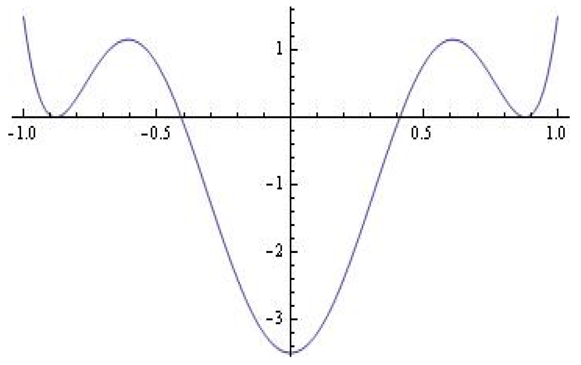
The Melnikov polynomial in (see Figure 8) gives:
□
The radii for some values of are tabulated in Table 2.
For an proper choice of the parameter (for example ), we have a limit cycle and limit cycle with multiplicity 2 (see Table 2). The solution of the system (8) for , , with , is visualized in Figure 9.
The case . Consider the model
where , . The following is correct:
Proposition 3.
The Lienard-type system (10) for , and for all small enough for , has 2 simple limit cycles and limit cycle with multiplicity–2.
The proof of existence of limit cycles is based on the ideas given in Propositions 1 and 2, and we will omit it here.
We note that for the Melnikov polynomial in (see Figure 10) we obtain:
The solution of the system (10) for , , with , is visualized in Figure 11.
2.3. Related Problems and Possible Applications
Let us explore the following Lienard system:
where .
Numerical examples
Example 1.
Example 2.
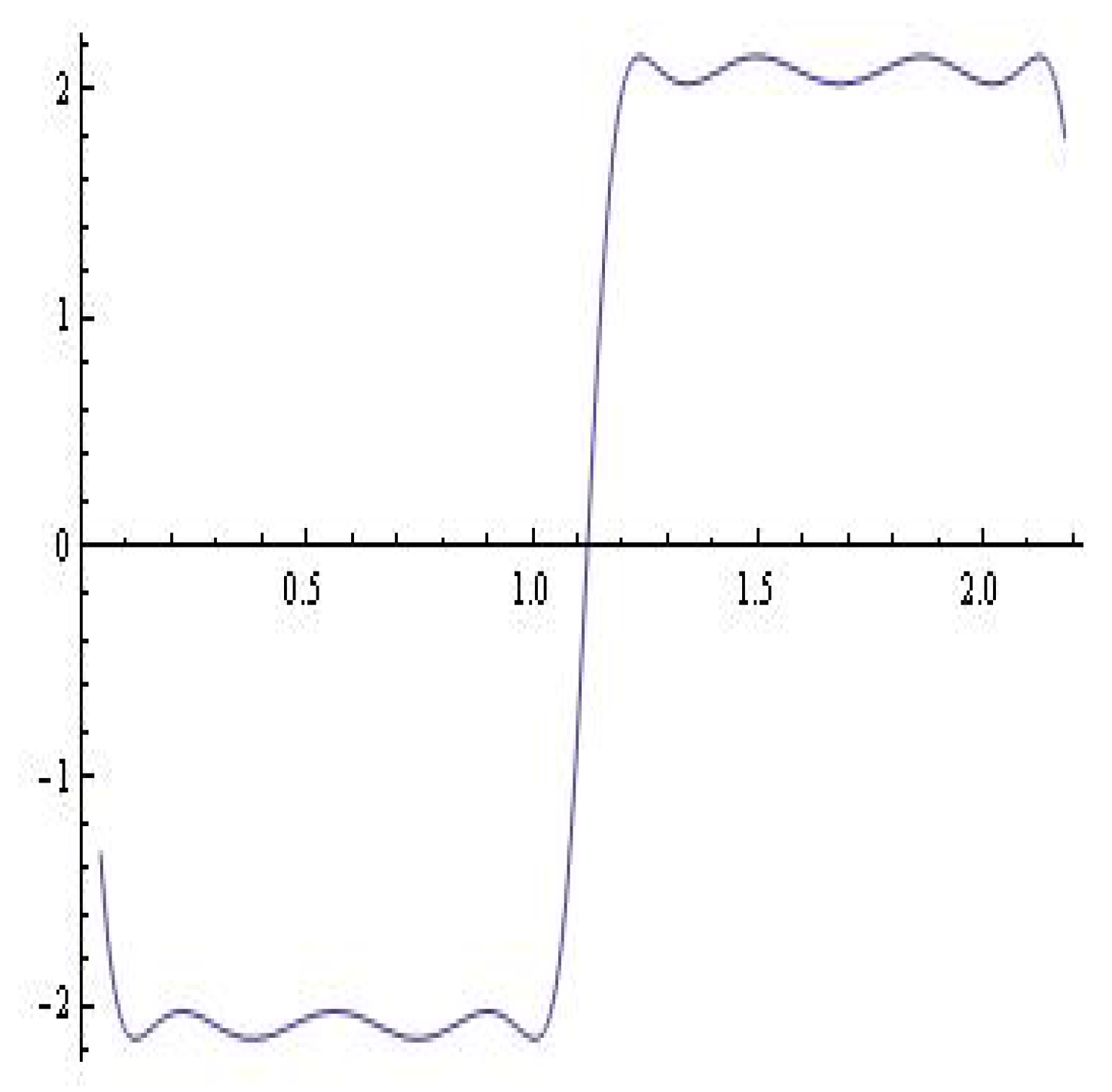
The solution of the system (12) for , , is visualized on Figure 13.
We will explicitly note that the -components of the differential systems discussed above can be used successfully in modeling and approximating functions and point sets in the field of signal theory, filters, and other characteristics.
Applications
We will consider 2 typical examples.
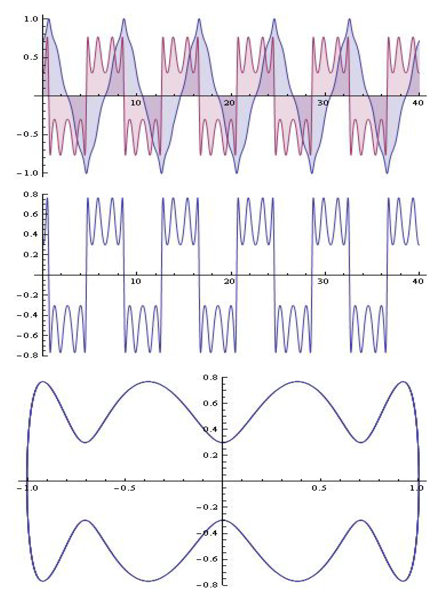
(A) Example 1 shows that the component of the solution of system (12) (with , ) can be used for the modeling and synthesis of electric circuits of the type shown in Figure 14 at an appropriately selected interval.
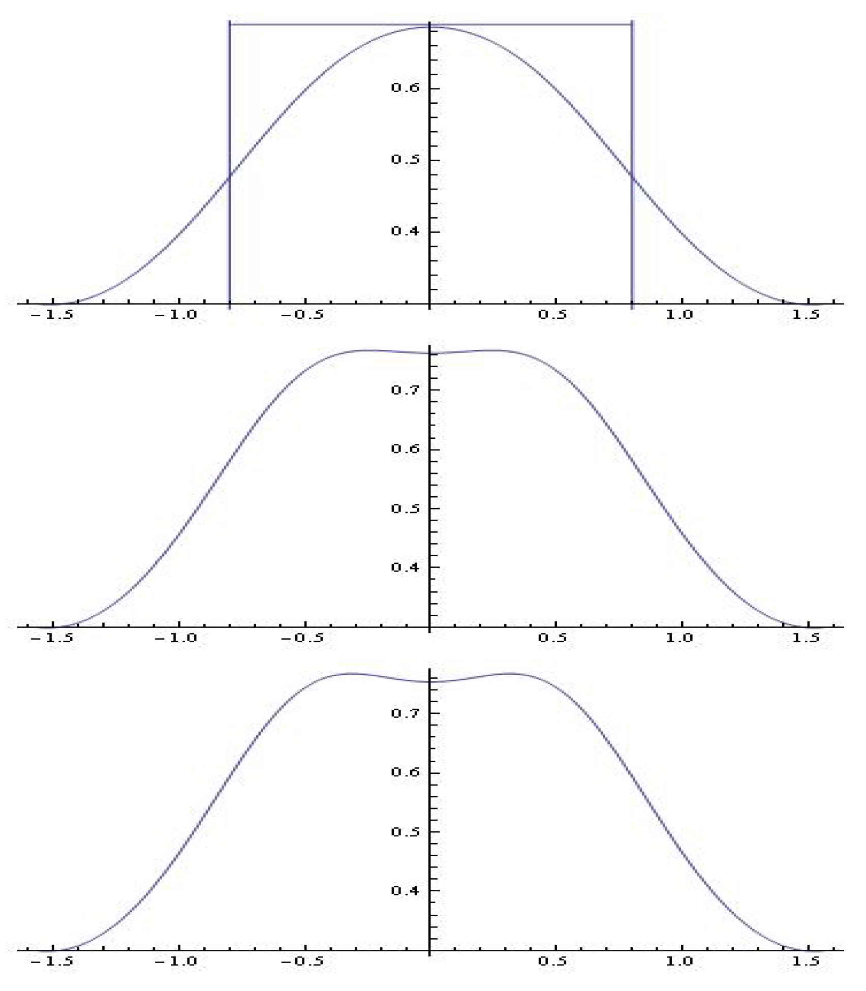
(B) A number of studies are known on the design of in some sense optimal filters, such as the exponential optimal filters of Tadmore and Tanner [8,9] (for the intrinsic properties of these filters concerning Hausdorff metrics, see [10]).
It is easy to take into account that the alteration of the variable t with in the y-component of the solution of the system (12) leads to a diagram characteristic of a filter.
By varying the parameter a, a variety of interesting models are obtained (see Figure 15).
3. Concluding Remarks
The reader can pin down the adequate approximation results for some n. For example, for fixed the Lienard system through Melnikov’s approach is defined as
The Melnikov polynomial is of the form (see Figure 16):
and the following statement is valid:
Proposition 4.
The Lienard-type system for has four simple limit cycles: , , , and and limit cycle with multiplicity–2.
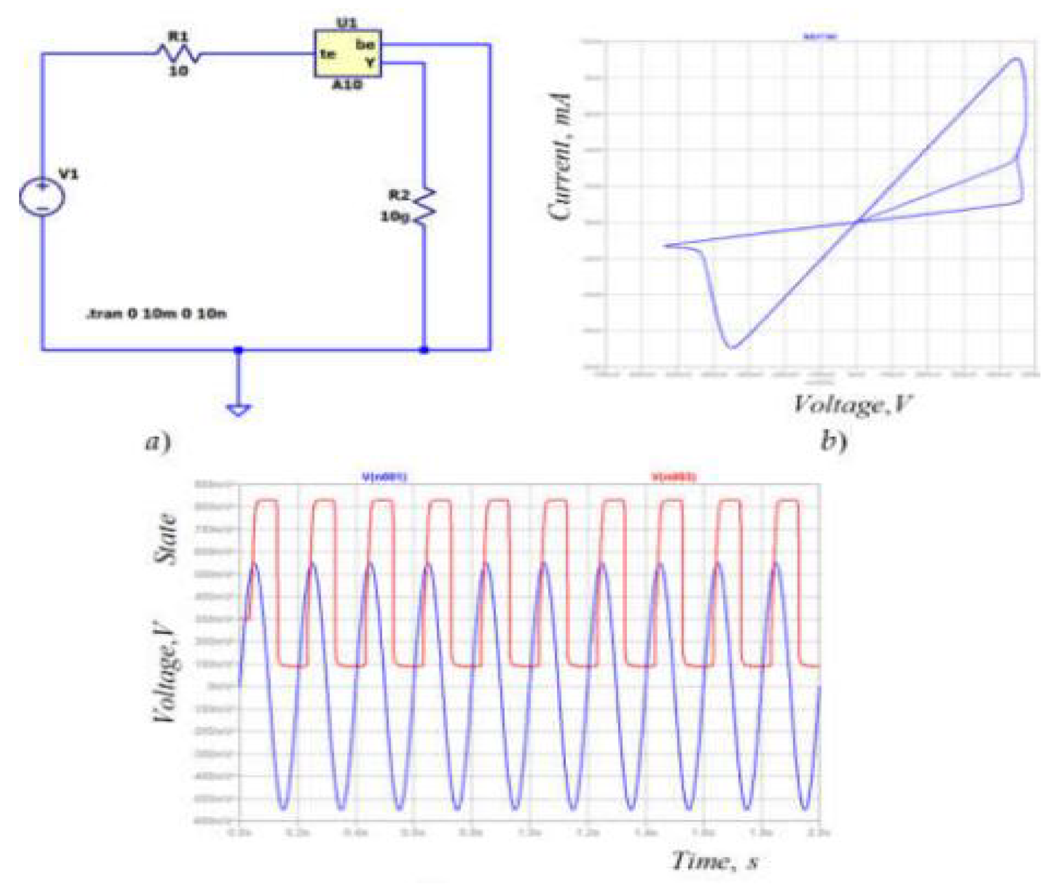
The topics in this paper are connected to solving some practical issues such as the synthesis of antennas and electrical circuits. For example, a simple circuit for testing the memristor model and corresponding current–voltage characteristics is given in [11], see Figure 17. For other results, see [11,12,13,14,15,16].
Intriguing radiation diagrams can be received with a proper selection of the functions and arising in the Lienard system. Interesting outcomes are obtained in [7,17,18,19,20].
Remark 1.
The study of dynamical systems includes bifurcation theory with branch catastrophe theory [21]. Arnold [22] discussed the catastrophes of the ADE classification, because of their relation with the Lie groups. Consider the following model in the light of Zeeman’s approach [23]:
with and
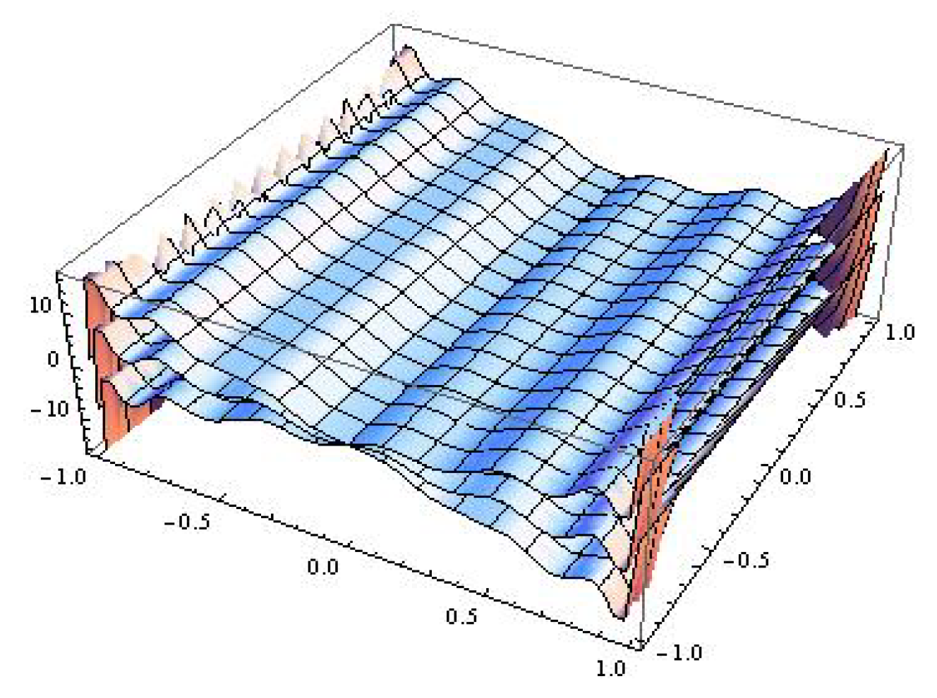
For the model the catastrophe surface is depicted in Figure 18.
3.1. Numerical Issues Connected to the Investigation of the Roots of the Melnikov Polynomial
Let be the polynomial with real and multiple roots with the multiplicities , where , i.e.,
The next theorem is fulfilled
Theorem 1
If the initial approximations of the zeros satisfy the inequalities , then the inequalities
hold true.
3.2. The Level Curves
For more details of the existing important results on the generalized polynomial Lienard differential systems and the limit-cycle bifurcations of some generalized polynomial Lienard systems, see [30,31,32,33,34,35,36,37,38,39,40,41,42,43,44,45,46,47].
Consider the class of Lienard polynomial systems of the type
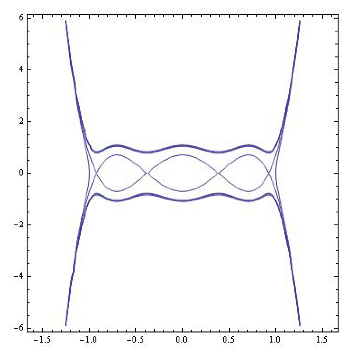
where ; (a) is the Chebyshev polynomial of the second kind and are bounded parameters. Without going into details, we will note some interesting level curves. For , system (14) is a Hamiltonian system with Hamiltonian
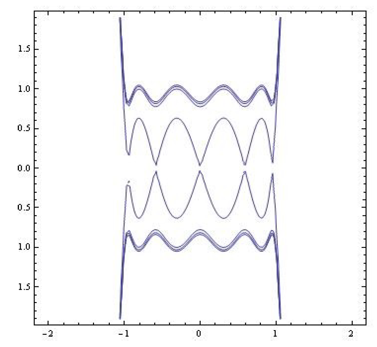
The level curves are depicted in Figure 19. The case b) . The Hamiltonian of system (14) () is
The level curves are depicted in Figure 20.
The outcomes received in this paper are based on the following algorithms:
(i) For the arbitrary order n fixed by the user—the production of the extended oscillator;
(ii) For the existence of the boundary cycle—the automatic checking of the rules in Lienard’s theorem;
(iii) For determining their number and type—receiving sure evaluations for the roots of the polynomial and the high-order Melnikov polynomials ;
(iv) For embedding polynomial-type rectification factors—generating dynamic models.
Software for study and depiction have also been produced, written in CAS Mathematica. These modules are improving similar ones realized in computer algebraic systems designed for scientific calculations. The offered modules are only part of the more general project for investigating nonlinear models.
Author Contributions
Conceptualization, N.K.; methodology, N.K.; software, A.I.; validation, N.K. and A.I.; formal analysis, N.K.; investigation, N.K.; resources, A.I.; data curation, N.K.; writing—original draft preparation, N.K.; writing—review and editing, A.I.; visualization, A.I.; supervision, N.K.; project administration, N.K.; and funding acquisition, A.I. All authors have read and agreed to the published version of the manuscript.
Funding
This work has been accomplished with the financial support of grant no BG05M2OP001-1.001-0003, financed by the Science and Education for Smart Growth Operational Program (2014–2020) and co-financed by the European Union through the European Structural and Investment Funds.
Institutional Review Board Statement
Not applicable.
Informed Consent Statement
Not applicable.
Data Availability Statement
Not applicable.
Acknowledgments
The authors would like to express their gratitude to the anonymous reviewers for their helpful comments and to the editors for suggestions that improved the quality and presentation of the paper.
Conflicts of Interest
The authors declare no conflict of interest.
References
- Hilbert, D. Mathematical problems (M.Newton Transl.). Bull. Am. Math. Soc. 1901, 8, 437–479. [Google Scholar] [CrossRef] [Green Version]
- Melnikov, V.K. On the stability of a center for time–periodic perturbation. Trudy Moskovskogo Matematicheskogo Obshchestva 1963, 12, 3–52. [Google Scholar]
- Lienard, A. Etude des oscillations entretenues. Revue Generale de e’Electricite 1828, 23, 901–912, 946–954. [Google Scholar]
- Blows, T.; Perko, L. Bifurcation of Limit Cycles from Centers and Separatrix Cycles of Planar Analytic Systems. SIAM Rev. 1994, 36, 341–376. [Google Scholar] [CrossRef]
- Perko, L. Differential Equations and Dynamical Systems; Springer: New York, NY, USA, 1991. [Google Scholar]
- Kyurkchiev, N.; Andreev, A. Approximation and Antenna and Filters Synthesis. Some Moduli in Programming Environment Mathematica; LAP LAMBERT Academic Publishing: Saarbrucken, Germany, 2014; 150p, ISBN 978-3-659-53322-8. [Google Scholar]
- Kyurkchiev, V.; Kyurkchiev, N. On an extended relaxation oscillator model: Number of limit cycles, simulations. I. Commun. Appl. Anal. 2022, 26, 19–42. [Google Scholar]
- Tadmor, E.; Tanner, J. Adaptive filters for piecewise smooth spectral data. IMA J. Numer. Alg. 2005, 25, 535–547. [Google Scholar] [CrossRef] [Green Version]
- Tanner, J. Optimal filter and mollifier for piecewise smooth spectral data. Math. Comput. 2006, 75, 767–790. [Google Scholar] [CrossRef] [Green Version]
- Kyurkchiev, N. Some Intrinsic Properties of Tadmor-Tanner Functions: Related Problems and Possible Applications. Mathematics 2020, 8, 1963. [Google Scholar] [CrossRef]
- Mladenov, V. A unified and open LTSPICE memristor model library. Electronics 2021, 10, 1594. [Google Scholar] [CrossRef]
- Mladenov, V.; Kirilov, S. A Neural Synapse Based on Ta2O5 Memristor. In Proceedings of the 2021 17th International Workshop on Cellular Nanoscale Networks and their Applications (CNNA), Catania, Italy, 29–30 September 2021. [Google Scholar] [CrossRef]
- Mladenov, V.; Kirilov, S. A Simplified Tantalum Oxide Memristor Model, Parameters Estimation and Application in Memory Crossbars. Technologies 2022, 10, 6. [Google Scholar] [CrossRef]
- Mladenov, V.M.; Zaykov, I.D.; Kirilov, S.M. Application of a Nonlinear Drift Memristor Model in Analogue Reconfigurable Devices. In Proceedings of the 2022 26th International Conference Electronics, Palanga, Lithuania, 13–15 June 2022; pp. 1–6. [Google Scholar]
- Mladenov, V. Advanced Memristor Modeling–Memristor Circuits and Networks; MDPI: Basel, Switzerland, 2019. [Google Scholar]
- Mladenov, V. Analysis and Simulations of Hybrid Memory Scheme Based on Memristors. Electronics 2018, 7, 289. [Google Scholar] [CrossRef] [Green Version]
- Kyurkchiev, V.; Iliev, A.; Rahnev, A.; Kyurkchiev, N. A technique for simulating the dynamics of some extended relaxation oscillator models. II. Commun. Appl. Anal. 2022, 26, 43–59. [Google Scholar]
- Kyurkchiev, V.; Iliev, A.; Rahnev, A.; Kyurkchiev, N. Another extended polynomial Lienard systems: Simulations and applications. III. Int. Electron. J. Pure Appl. Math. 2022, 16, 55–65. [Google Scholar]
- Kyurkchiev, V.; Iliev, A.; Rahnev, A.; Kyurkchiev, N. Investigations on some polynomial Lienard-type systems: Number of limit cycles, simulations. Int. J. Differ. Equ. Appl. 2022, 21, 117–126. [Google Scholar]
- Kyurkchiev, V.; Kyurkchiev, N.; Iliev, A.; Rahnev, A. On Some Extended Oscillator Models: A Technique for Simulating and Studying Their Dynamics; Plovdiv University Press: Plovdiv, Bulgaria, 2022; ISBN 978-619-7663-13-6. [Google Scholar]
- Beltrami, E. Mathematics for Dynamic Modeling; Academic Press: Boston, MA, USA, 1987. [Google Scholar]
- Arnold, V. Geometrical Methods in the Theory of Ordinary Differential Equation; Springer: Berlin/Heidelberg, Germany, 1988. [Google Scholar]
- Zeeman, E. Catastrophe Theory. Selected Papers 1972–1977; Addison-Wesley: Reading, MA, USA, 1977. [Google Scholar]
- Kyurkchiev, N.; Andreev, A.; Popov, V. Iterative methods for the computation of all multiple roots of an algebraic polynomial. Annu. Univ. Sofia Fac. Math. Mech. 1984, 78, 178–185. [Google Scholar]
- Proinov, P.; Vasileva, M. On the convergence of high-order Ehrlich-type iterative methods for approximating all zeros of a polynomial simultaneously. J. Inequalities Appl. 2015, 2015, 336. [Google Scholar] [CrossRef]
- Proinov, P.D.; Vasileva, M.T. Local and Semilocal Convergence of Nourein’s Iterative Method for Finding All Zeros of a Polynomial Simultaneously. Symmetry 2020, 12, 1801. [Google Scholar] [CrossRef]
- Kyncheva, V.; Yotov, V.; Ivanov, S. Convergence of Newton, Halley and Chebyshev iterative methods as methods for simultaneous determination of multiple zeros. Appl. Numer. Math. 2017, 112, 146–154. [Google Scholar] [CrossRef]
- Petkovic, I.; Herceg, D. Computer methodologies for comparison of computational efficiency of simultaneous methods for finding polynomial zeros. J. Comput. Appl. Math. 2020, 368, 112513. [Google Scholar] [CrossRef]
- Kanno, S.; Kjurkchiev, N.; Yamamoto, T. On some methods for the simultaneous determination of polynomial zeros. Jpn. J. Appl. Math. 1995, 13, 267–288. [Google Scholar] [CrossRef]
- Llibre, J.; Valls, C. Global centers of the generalized polynomial Lienard differential systems. J. Differ. Equ. 2022, 330, 66–80. [Google Scholar] [CrossRef]
- Chen, H.; Lie, Z.; Zhang, R. A sufficient and necessary condition of generalized polynomial Lienard systems with global centers. arXiv 2022, arXiv:2208.06184. [Google Scholar]
- He, H.; Llibre, J.; Xiao, D. Hamiltonian polynomial differential systems with global centers in the plane. Sci. China Math. 2021, 48, 2018. [Google Scholar]
- Smale, S. Mathematical problems for the next century. Math. Intell. 1998, 20, 7–15. [Google Scholar] [CrossRef]
- Zhao, Y.; Liang, Z.; Lu, G. On the global center of polynomial differential systems of degree 2k + 1. In Differential Equations and Control Theory; CRC Press: Boca Raton, FL, USA, 1996; 10p. [Google Scholar]
- Andronov, A.A.; Leontovich, E.A.; Gordon, I.I.; Maier, A.G.; Gutzwiller, M.C. Qualitative Theory of Second Order Dynamic Systems; Wiley: New York, NY, USA, 1973. [Google Scholar]
- Hale, J.K. Ordinary Differential Equations; Wiley: New York, NY, USA, 1980. [Google Scholar]
- Garcia, I.A. Cyclicity of Nilpotent Centers with Minimum Andreev Number. 2019. Available online: https://repositori.udl.cat/handle/10459.1/67895 (accessed on 1 October 2022).
- Sun, X.; Xi, H. Bifurcation of limit cycles in small perturbation of a class of Lienard systems. Int. J. Bifurc. Chaos 2014, 24, 1450004. [Google Scholar] [CrossRef]
- Asheghi, R.; Bakhshalizadeh, A. On the distribution of limit cycles in a Lienard system with a nilpotent center and a nilpotent saddle. Int. J. Bifurc. Chaos 2016, 26, 1650025. [Google Scholar] [CrossRef]
- Zaghian, A.; Kazemi, R.; Zangenech, H. Bifurcation of limit cycles in a class of Lienard system with a cusp and nilpotent saddle. UPB Sci. Bull. Ser. A 2016, 78, 95–106. [Google Scholar]
- Gaiko, V.; Vuik, C.; Reijm, H. Bifurcation Analysis of Multi–Parameter Lienard Polynomial System. IFAC-PapersOnLine 2018, 51, 144–149. [Google Scholar] [CrossRef]
- Cai, J.; Wei, M.; Zhu, H. Nine limit cycles in a 5-degree polynomials Lienard system. Complexity 2020, 2020, 8584616. [Google Scholar] [CrossRef]
- Xu, W.; Li, C. Limit cycles of some polynomial Lienard system. J. Math. Anal. Appl. 2012, 389, 367–378. [Google Scholar] [CrossRef]
- Xu, W. Limit cycle bifurcations of some polynomial Lienard system with symmetry. Nonlinear Anal. Differ. Equ. 2020, 8, 77–87. [Google Scholar] [CrossRef]
- Hou, J.; Han, M. Melnikov functions for planar near–Hamiltonian systems and Hopf bifurcations. J. Shanghai Norm. Univ. (Nat. Sci.) 2006, 35, 1–10. [Google Scholar]
- Han, M.; Yang, J.; Tarta, A.; Gao, Y. Limit cycles near homoclinic and heteroclinic loops. J. Dyn. Differ. Equ. 2008, 20, 923–947. [Google Scholar] [CrossRef]
- An, Y.; Han, M. On the number of limit cycles near a homoclinic loop with a nilpotent singular point. J. Differ. Equ. 2015, 258, 3194–3247. [Google Scholar] [CrossRef]
Figure 1.
for , and .

Figure 2.
The system solutions (; ).

Figure 3.
The system solutions (; ).

Figure 4.
The system solutions (; ).

Figure 5.
The system solutions (; ).

Figure 6.
for and .

Figure 7.
(a) The solutions of the system (6) (; ; ); (b) the portrait ; (c) 3D plot.

Figure 8.
for and . The roots are: —simple and —with multiplicity 2.

Figure 9.
(a) The solutions of the system (8) (; ; ); (b) the portrait ; (c) 3D plot.

Figure 10.
for and . The simple roots are , and root —with multiplicity 2.

Figure 11.
The solutions of the system (10) (; ; ).

Figure 12.
The solutions of the system (12) (Example 1).

Figure 13.
The solutions of the system (12) (Example 2).

Figure 14.
Application for modeling and analysis of electrical circuits and signal processes.

Figure 15.
The model for , in for (a) ; (b) ; and (c) .

Figure 16.
The Melnikov polynomial .

Figure 17.
A simple circuit for testing the memristor model and corresponding current–voltage characteristics [11].
Figure 17.
A simple circuit for testing the memristor model and corresponding current–voltage characteristics [11].

Figure 18.
The catastrophe surface ; .

Figure 19.
The level curves (the case a).

Figure 20.
Level curves (the case b).


Table 1.
The radii for some values of .
| 5 | 0.518013 | 0.965227 |
| 6 | 0.595862 | 0.919211 |
| 7 | 0.707107 | 0.83666 |
| 7.2 | 0.774597 | 0.774597 |
Table 2.
The values of that proceed in 3 positive zeros of the Melnikov polynomial (Theorem 2); for : a simple limit cycle and limit cycle with multiplicity–2.
Table 2.
The values of that proceed in 3 positive zeros of the Melnikov polynomial (Theorem 2); for : a simple limit cycle and limit cycle with multiplicity–2.
| 7.5 | 0.433391 | 0.808263 | 0.934435 |
| 7.3 | 0.423255 | 0.826862 | 0.922735 |
| 7.1 | 0.413469 | 0.851545 | 0.904544 |
| 7.008805257 | 0.409106 | 0.878462 | 0.879469 |
Publisher’s Note: MDPI stays neutral with regard to jurisdictional claims in published maps and institutional affiliations. |
© 2022 by the authors. Licensee MDPI, Basel, Switzerland. This article is an open access article distributed under the terms and conditions of the Creative Commons Attribution (CC BY) license (https://creativecommons.org/licenses/by/4.0/).
Share and Cite
MDPI and ACS Style
Kyurkchiev, N.; Iliev, A. On a Hypothetical Model with Second Kind Chebyshev’s Polynomial–Correction: Type of Limit Cycles, Simulations, and Possible Applications. Algorithms 2022, 15, 462. https://doi.org/10.3390/a15120462
AMA Style
Kyurkchiev N, Iliev A. On a Hypothetical Model with Second Kind Chebyshev’s Polynomial–Correction: Type of Limit Cycles, Simulations, and Possible Applications. Algorithms. 2022; 15(12):462. https://doi.org/10.3390/a15120462
Chicago/Turabian StyleKyurkchiev, Nikolay, and Anton Iliev. 2022. "On a Hypothetical Model with Second Kind Chebyshev’s Polynomial–Correction: Type of Limit Cycles, Simulations, and Possible Applications" Algorithms 15, no. 12: 462. https://doi.org/10.3390/a15120462
Note that from the first issue of 2016, this journal uses article numbers instead of page numbers. See further details here.