
Efficiency of Algorithms for Computing Influence and Information Spreading on Social Networks


1
Finnish Defence Research Agency, Tykkikentäntie 1, P.O. Box 10, 11311 Riihimäki, Finland
2
Eficode Oy, 00100 Helsinki, Finland
3
Department of Computer Science, Aalto University School of Science, P.O. Box 15500, 00076 Aalto, Finland
4
The Alan Turing Institute, 96 Euston Rd, Kings Cross, London NW1 2DB, UK
*
Author to whom correspondence should be addressed.
†
These authors contributed equally to this work.
Algorithms 2022, 15(8), 262; https://doi.org/10.3390/a15080262
Submission received: 30 June 2022
/
Revised: 20 July 2022
/
Accepted: 25 July 2022
/
Published: 28 July 2022
(This article belongs to the Special Issue Scalable Programming Models and Algorithms for Big Data)
Abstract
:Modelling interactions on complex networks needs efficient algorithms for describing processes on a detailed level in the network structure. This kind of modelling enables more realistic applications of spreading processes, network metrics, and analyses of communities. However, different real-world processes may impose requirements for implementations and their efficiency. We discuss different transmission and spreading processes and their interrelations. Two pseudo-algorithms are presented, one for the complex contagion spreading mechanism using non-self-avoiding paths in the modelling, and one for simple contagion processes using self-avoiding paths in the modelling. The first algorithm is an efficient implementation that can be used for describing social interaction in a social network structure. The second algorithm is a less efficient implementation for describing specific forms of information transmission and epidemic spreading.
1. Introduction
Modern information communication technology (ICT) together with social media services provides us with easy ways to be in contact, communicate, and interact with other people as well as means to exert influence on them. These acts lead to the formation of socially connected and dynamically changing groups, communities, and societies, which can be visualised as social networks of individuals considered as nodes and interactions between them as links with weights. These links are not limited to kin and friends in one’s own proximity, but also to people in far-away locations and with different cultures that make the social network structurally complex and distance-independent at a large scale. This reflects behavioural, socioeconomic, and societal changes, thus making the spreading, exchange, and sharing of information, opinion, and influence, easier and faster. In these acts and events, a lot of data is generated and stored, which through data analysis and data-driven modelling can give us qualitative and quantitative insight into the structure of and dynamics in social networks.
1.1. Influence and Information-Spreading Mechanisms
In general, a research approach based on networks and their modelling offers theoretical means to study social phenomena due to the fact that different kinds of relationships and influence between social actors can be represented [1,2,3,4,5]. A good example is diffusion in a network, which can be viewed as the process of information, influence, or disease spreading from one actor to another [6,7]. While each of the aforementioned processes describes a different phenomenon of human behaviour, they share common features in their transmission mechanisms. They all are manifestations of interactions and consequences of contacts between individuals in social networks. The transmission of information and the spread of social influence are two processes that usually do not exist in their pure form. In the case of a disease that spreads through contacts between individuals, the probability of the disease spreading correlates with the strength and frequency of social interactions between people.
Social media and interactive digital channels allow us to create and share information, ideas, interests, and other forms of expression through virtual communities and networks. It is common for models that one piece of information may only be mediated once between two individuals, but in practice, information is not presented in a normalised form like structural data in a database [8]. Unstructured data is presented in text or multimedia formats of different sizes and dimensions. Even if we could normalise some of the data items, a great deal of the information is unstructured, descriptive, or uncertain. It may even include misinformation or fake news. We thus propose that recurrent and repeated mechanisms describe the spreading processes in both structured and unstructured information transmission.
Rogers [9] has studied the diffusion of innovations and communication processes, where communication is described as a process in which participants create and share information. It is a two-way process in which an individual seeks to transfer a message to another in order to achieve wanted effects. Communication is a convergent process as when two or more individuals exchange information, they will eventually reach a stable state of mutual understanding. In human communication processes, information is exchanged between a pair of individuals and the spread of information may continue through several cycles. Rogers [9] defines diffusion as communication in which messages are new ideas or innovations. Communication processes, as defined in [9], and influence spreading processes, studied in our work [6,7], are two closely related concepts.
Influence spreading entails various methods of interactions that can change people’s opinions [10], behaviour [11], and beliefs [12] and it can be characterised as a continuous psychological process rather than a chain of nonrecurring information transmission events. People gather together and influence each other in different situations and environments, for example, in families, workplaces, and hobbies. Many diseases, such as viruses, spread through physical contacts, the air, or other transmitting media. It is clear that social interactions are correlated with epidemic-spreading mechanisms. If the only transmission channel of disease is through physical contact, the spreading process can be considered to be similar to the information-transfer mechanism.
Traditionally, models of social and biological contagion have been classified into two categories: simple and complex contagion. Simple contagion describes spreading processes induced by a single exposure, while complex contagion requires multiple sources of exposure before an individual adopts a change of behaviour [11,12,13]. Recently, the need for generalised contagion models has been discussed and a unifying model has been presented [14]. Furthermore, models of opinion dynamics in social networks have been classified into models with discrete or continuous opinions [10]. influence spreading models proposed in this study are continuous models as the opinion state variables of our model take continuous probability values.
In this study, differing from the definition of [11], we categorise the case of processes using self-avoiding paths as simple contagion (SC) processes while all other alternatives are considered complex contagion (CC) processes. If loops are allowed, one node can be visited several times during the spreading process. If loops are not allowed, we say that only self-avoiding paths are possible.
In summary, we can say that different versions of complex contagion are more common in describing real-world phenomena. An SC model using self-avoiding paths does not allow breakthrough influence [7] and is used for describing information transfer in a specific case of spreading normalised data items by agents with memory. Additionally, SC models can be used to describe specific virus epidemics with immunisation.
The methodology for modelling and analysing influence spreading, human behaviour and interaction with others in a social network has been published in our earlier studies [6,7]. Here, we focus on presenting the explicit pseudo-algorithms in a form that enables researchers to implement and further develop the models. In addition, we discuss the efficiency and application areas of the methods. We provide examples of the modelling results for two networks of different sizes: a social media network and a social network.
1.2. Algorithms Using Non-Self-Avoiding Paths vs. Self-Avoiding Paths
Modelling interactions in complex networks needs efficient algorithms for describing processes at a detailed level and on a global scale in the network. This kind of modelling enables more realistic applications of spreading processes, network metrics, and analyses of communities. In this paper, we will discuss different transmission and spreading processes and their interrelations.
In Section 2.2.1 and Section 2.2.2, we will present two different versions of the influence spreading model. The complex contagion algorithm is an implementation for describing social influence interactions, and the simple contagion algorithm is proposed primarily for applications to model information spreading and virus epidemics. After all, contagion processes often occur with competition between simple and complex contagion, as explained in [14].
The complex contagion algorithm is a scalable and efficient algorithm [15] proposed for computing an influence spreading matrix [6] that can be used as an input for computing various derived quantities and constructs, such as centrality measures and community structures. Social interactions can be considered as complex contagion processes on social networks with non-self-avoiding paths. The simple contagion algorithm is an example of a less efficient algorithm that is needed to describe specific forms of transmission processes in networks with self-avoiding paths.
2. Methods
2.1. Influence Spreading Model
In this section, we describe the influence spreading model [6] that is at the core of the presented algorithms. A similar model, called Independent Cascade Model, was presented by Kempe et al. [16] Our model may be viewed as a generalisation of the Independent Cascade Model, which does not allow self-intersecting paths or breakthrough influence.
The model describes a form of diffusion in a social network, and it is based on assigning a spreading probability to each edge of the network. Diffusion starts from a specified starting node, and each node has one chance to spread influence to each of the neighbouring nodes with the probability specified by the assigned edge probabilities.
We store all pairwise spreading probabilities in a two-dimensional influence spreading matrix , where denotes the probability of spreading from the starting node s to the target node t. The matrix elements are computed based on all possible paths between the corresponding pair of nodes. In other words, for computing , we will combine the influence of all paths from node s to node t. It is important to note that and will not always be equal as probabilities are assigned to each directed edge individually. Notice that paths between two nodes may have arbitrarily many nodes when we place no restrictions on them. Thus, to keep the set of paths finite, we need to limit path length. Let denote the maximum number of edges allowed on a path.
In addition to edge-specific probabilities, Poisson distribution is used to model temporal spreading. It is applied as a factor to the probability of spreading through a path. The Poisson distribution is a discrete probability distribution that expresses the probability for a giving a number of events occurring in a fixed interval of time provided that these events take place with a known constant rate and independently of the time since the previous event. In this context, the Poisson process describes a process where spreading via successive links occurs randomly as a function of time [6]. The unconditional probability of temporal spreading at time T on a path of length L is given by
where is the intensity parameter of the Poisson distribution. and T are constants throughout the calculation. Here, the interpretation is that the spreading has advanced up to L or more links at time T [6]. When , the values of approach to one. Additionally, other path length-dependent distributions could be used to more accurately model the different kinds of real-world influence spreading.
Now, we are ready to calculate the probability of a single spreading path. Let denote the probability of spreading through path , starting from the first node and traversing the path through each edge until the end. is the product of corresponding edge probabilities and the Poisson distribution coefficient from Equation (1); that is,
where denotes the spreading probability through the edge from u to v, the set of edges on path , and the size of the edge set; that is, the number of edges on the path [6].
To combine the probabilities of two different paths and between the same pair of nodes, we let denote the longest common prefix (LCP) of the paths. If there are no common nodes, i.e., is an empty path, we say that . Otherwise, let us derive a formula for calculating from and . We assume that the probabilities of two paths, after the first diversion, become unconditional and that the probabilities of non-intersecting paths are not dependent on each other. As a node can be influenced only once, we have to subtract the possibility that influence spreads through both and . Now [6],
The probability of spreading from node s to node t, , is calculated by combining all paths from node s to node t. If there are no paths from node s and to t, we say that . To ensure that the common prefixes of paths are combined correctly, we require that the paths are sorted lexicographically by their nodes, and that only adjacent paths are combined—in decreasing order of the number of common prefix nodes. Eventually, paths with no common links are combined until there is only one path left. The last path’s spreading probability is interpreted as the probability of influence spreading between the nodes. The process of combining paths is described in more detail in Algorithm 1. While it is a simplified version of the model and inefficient for most of the real-world network sizes, it serves as a foundation for our algorithms and provides a base model to implement more efficiently.
An important aspect of our algorithm is that nodes have no state during the path-merging process. This is in contrast to the independent cascade model [16], where each node, after activating has one chance to spread influence to each of its inactive neighbours, after which the node becomes active, and will not spread influence again. Even though we can restrict the search to self-avoiding paths, that is to paths where each node only appears once, we are not able to take control of breakthrough influence, i.e., influence through a node that has been influenced before. The fact that the nodes have no state is one of the reasons our algorithm is efficient. However, this difference means that our model and the independent cascade model are for describing distinctly different real-world phenomena.
| Algorithm 1 The path combination process [7] |
|
Because the model is built on top of the concept of spreading paths, we are able to reduce the search space by limiting path length. In addition to making computation more efficient, this allows for studying the influence of a node in its local neighbourhood, rather than studying its position in the global structure of the network.
2.2. Algorithms
In this section, we present two algorithms, Algorithms 2 and 3 which both implement the logic of Algorithm 1. While they are more efficient than the original algorithm, they still combine paths in the same manner and output the same values. The path combination process, more precisely the order in which paths are combined, is present in all algorithms, but readers may find it harder to grasp in the more efficient implementations below.
2.2.1. Complex Contagion Algorithm
First, we describe an efficient algorithm for modelling complex contagion (CC). In the case of complex contagion, self-intersecting paths are allowed. Algorithm 2 solves this problem for a fixed target node t. To fill the influence spreading matrix, the procedure needs to be run times, once with each node as the target node. As mentioned, represents the maximum path length, that is, the number of edges on a path.
Two important factors contribute to the algorithm’s efficiency. Firstly, no restrictions, other than the maximum path length, are posed on paths. A spreading path may, for example, self-intersect. This means that we do not need to have the current path in memory in order to select the next node. Instead, it suffices to store the latest node and the length of the path. This allows us to save memory by grouping multiple paths together and combining their probabilities during the computation, rather than storing all individual paths until the end. Secondly, nodes have no state; that is, they are neither influenced nor uninfluenced. This means that we need not store the state of each node in memory nor do we need to process a great number of possible states individually.
| Algorithm 2 The Complex Contagion algorithm |
|
| Algorithm 3 The Simple Contagion Algorithm |
|
The algorithm works backwards, building paths starting from the target node t, which is the last node on all paths. The backwards computation ensures that all pairs of paths are combined at the latest possible node as required by the model. The node, at which a pair of paths is combined, is the one where the paths diverge from each other for the first time. Spreading probabilities are stored in a two-dimensional array P, where corresponds to all paths with latest node i and L nodes missing. After calculations are finished, , i.e., paths ending at i with no nodes left, stores the probability of spreading from i to t. The value of is calculated by combining the values of for all j which are connected to i. At each step, we are essentially continuing all started paths backwards through all possible edges.
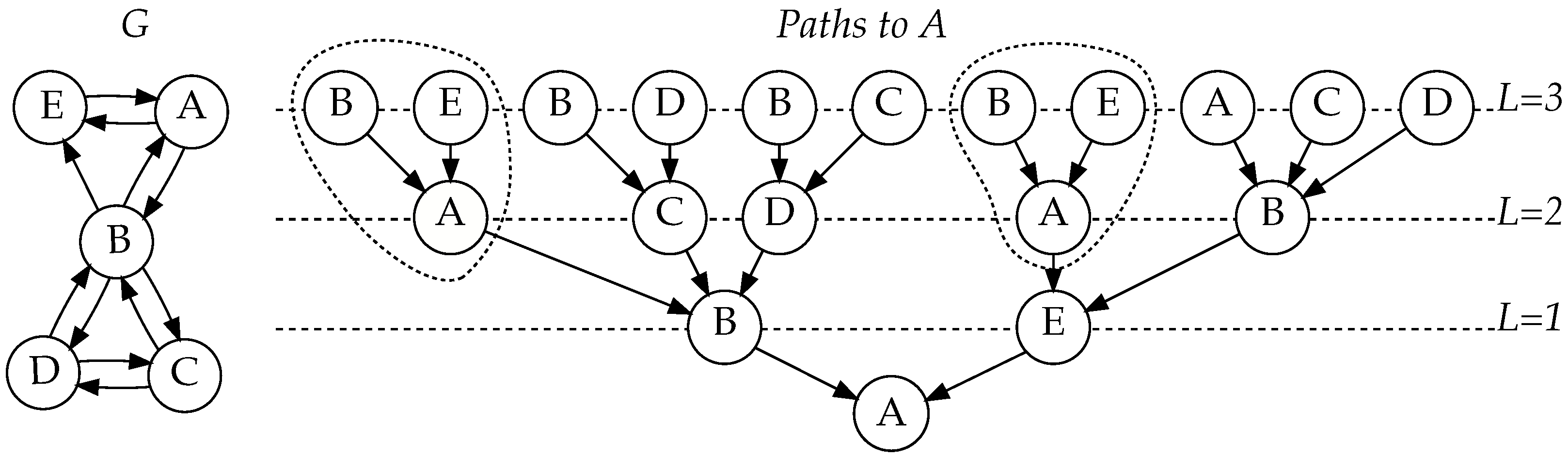
In Figure 1, notice how length-one paths ending at A are used in two different contexts. They are extended with edges and separately (circled in Figure 1). Because, in the previous round, we have already computed and cached the value for , we can use it in multiple contexts without needing to compute it again.
Before the computation, is initialised with the corresponding Poisson factor from Equation (1). Next, iterations follow, numbered from to 0. In iteration i, new paths are started from t, and already started paths obtain their -th node. For example, in the first iteration, when , paths of length obtain their second to last node and paths of length are started from t, with t as their -th node.
For a fixed end node, the algorithm works in time, where E denotes the number of edges in the network and the maximum allowed path length (measured in edges), making the total time complexity of solving the influence spreading matrix . The runs can easily be distributed to different cores or computation units as the calculations are completely independent, making the algorithm highly parallelisable. Moreover, the innermost loop’s iterations are also independent from each other, and can thus be parallelised, on the CPU instruction level. These factors combined make running the algorithm highly efficient in practice.
Memory-wise, the algorithm scales well for large networks as, at any time, we only need the values corresponding to the two latest values of L. Thus, we need to store two floating point numbers for each node per run, making the memory complexity of a single run .
2.2.2. Simple Contagion Algorithm
The second algorithm (Algorithm 3) known as the simple contagion(SC) algorithm models self-avoiding spreading. In self-avoiding spreading, paths must be non-intersecting. To avoid choosing a node which is already on the path, we must have the current path in memory, which slows down the computation significantly.
The algorithm itself is a recursive depth-first search, which goes through all possible paths with a suitable length. The search starts from the given starting node s and recursively traverses to each neighbouring node. At any point, the current stack of recursive calls corresponds to the current path prefix. Provided there are no duplicate edges, each possible prefix is only seen once. All paths which have the current call stack as their prefix are constructed either in the current function call or in the subsequent recursive calls inside of it.
Algorithm 3 uses the technique from Equation (3) for combining paths and meets the model’s requirement that paths need to be combined at the end of their common prefix by, at each node, only constructing paths which first diverge at the node. Any pair of two differing paths has a specific node which corresponds to the end of the common prefix, which means that the procedure will, in fact, construct all possible paths—once and only once.
Each call to the depth-first search function has its own probability array P, which holds the probabilities spread to all other nodes. denotes the probability of spreading from the current node to node i. The values of depend on the current depth and thus cannot be used for calculating spreading probabilities from other starting nodes. After the probabilities for a node’s neighbours are recursively computed, they are combined into the probability array of the current node.
Note that were we to remove the self-avoiding restriction from line 9 of Algorithm 3, the algorithm would compute exactly the same values as the CC algorithm (Algorithm 2), but less efficiently. Another notable difference to the CC algorithm is that a single call to the SC algorithm (Algorithm 3) computes probabilities of spreading from a fixed start node s, while a single call to the CC algorithm calculates the values for a fixed end node.
It is well known that, in the worst case, there are paths with a fixed starting node and at most edges in a network of V nodes. The search function in Algorithm 3 updates the spreading probability of all nodes after processing each neighbour, making the total time complexity of a single run as each node has at most neighbours to process and there are nodes with a probability to update. As before, this algorithm needs to be run times, which increases the time complexity to fill the influence spreading matrix to . Both the SC algorithm and the original Algorithm 1 go through all spreading paths, but the fact that the SC algorithm does not store them in memory makes it significantly faster, more memory-efficient, and even usable in practice. It is scalable to large graphs with small values of . As was the case with Algorithm 2, the independent runs of this algorithm needed to fill the influence spreading matrix can be run in parallel to make computation more efficient. Combining the results of the runs is trivial, as each run corresponds to a single row in the final influence spreading matrix.
2.3. Applications
Probably the two most important subjects of complex networks are studying influence or information spreading and community detection. Spreading processes can be studied by analysing the influence spreading matrix and its elements . The influence spreading matrix is the end result of Algorithms 2 and 3 in Section 2.2.1 and Section 2.2.2, respectively. Elements of the matrix describe spreading probabilities between all ordered pairs of two nodes in the network structure.
The influence spreading matrix can be used in many network applications and in defining different network metrics. Here, we provide a short summary of the most important quantities: in- and out- centrality measures, a betweenness measure, and a quality function for community detection.
2.3.1. In- and Out-Centrality Measures
We define non-normalised in-centrality and out-centrality measures [6] for nodes s and t in a network with node set V as follows
Normalised versions of these quantities can be obtained by dividing the expressions by . These sums do not take the probability for a node to influence itself, which is always 1.0, into account. It follows that the centrality of an unconnected node is always 0.0. As individual values of the influence spreading matrix C correspond to spreading probabilities, by the linearity of expectation, the in-centrality sum from Equation (4) corresponds to the expected number of nodes that will influence a node and the out-centrality sum from Equation (5) to the number of nodes a node will influence. The interpretation of the presented centrality methods as expected values is crucial as it makes them physical quantities. In the literature, different methods for calculating centrality measures [17,18,19] have been proposed but they have no probabilistic interpretation nor are they based on detailed descriptions of networks.
2.3.2. Betweenness and Cohesion Measures
Next, we will define a betweenness centrality measure for our model. Betweenness centrality measures the ability of a node to mediate influence between nodes in the network. We let denote the betweenness centrality [6] of a single node m and , the betweenness centrality for a set of nodes M. is defined as the proportional change in cohesion when we remove the set of nodes M from the network structure, that is
where the cohesion B of the whole network is defined as the sum
is calculated similarly to B with the set of nodes M removed from the network structure as
where is the influence spreading matrix corresponding to a new graph with the set of nodes M removed.
Our measure differs from the classical definition of betweenness centrality [20,21,22] where the betweenness centrality of a node is defined by the number of shortest paths that pass through the node divided by the number of all shortest paths between pairwise nodes in the network. By contrast, Equation 6) considers all possible interactions and paths in the network. This is an important distinction to make as a lot of the structure of the graph is left out when we consider only the edges on the shortest paths from a node. In addition to giving more accurate numerical results, our definition is more general in the sense that it is independent of the network model and spreading mechanism, because Equation (6) is based only on matrices B and that can be calculated for different spreading or connection mechanisms of the network.
2.3.3. Community Detection Applications
The influence spreading matrix can be used for community detection. We define the quality function, or objective function, for detecting sub-communities as [6]
The quantity Q in Equation (9) is maximised to detect partitions into two sets of nodes, and in the network of nodes V. Note that cross-terms where s and t are not part of the same faction have no effect in Equation (9) which is typical for community detection methods in general [1,2]. The method can be generalised for more than two factions but, in practise, the method provides similar results by searching different local maxima of the quality function just for two factions. Because the number of cross-terms increases with the number of factions, there is no guarantee for more realistic results.
Other partitioning methods and quality functions, using the influence spreading matrix, than Equation (9) could be used for detecting the community structure. The form of Equation (9) is the simplest one, which can be used if any other mathematical form of the quality function is not specified in the application. There is no universal formulation of the quality function for community detection nor is there a commonly accepted definition of a community [23,24].
There are many areas of future research where the proposed framework based on the influence spreading matrix can be utilised. They include analysing dynamic network structures, different network models, temporal spreading distributions, signed networks, community detection based on locally dense subgraphs, and selecting optimal team members from a social network.
3. Case Study Results
In this section, we provide examples of how the model and its applications function in practice. We also provide insight into the effects of the maximum path length and how much it can be limited.
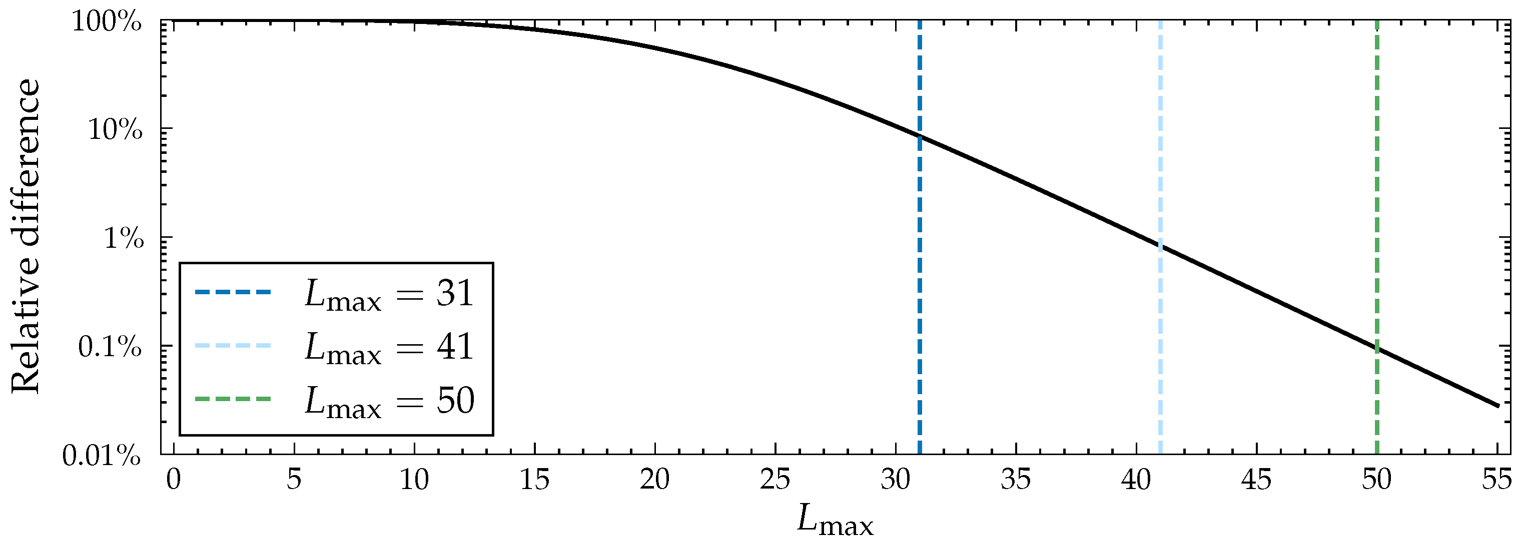
As mentioned, from a computational point of view, it is ideal to limit path length as much as possible in order to make the program run faster. Because the probability of spreading through a path decreases exponentially with respect to path length, the spreading probabilities eventually converge. Values in the influence spreading matrix approach the converged ones rather quickly, and after a point, increases in path length cause unnoticeable differences in the final probabilities. In the case of the Facebook network (see Figure 2) from the SNAP dataset [25], a dense graph of 4039 nodes and 88,234 edges, is the first value with which all out-centrality values differ by less than ten percent from the converged ones. At , the values differ by less than a percent, and at , by less than . The Facebook network used here is an example of a relatively large and dense network, which increases the amount of CC paths. In a more typical, sparser network, even smaller values of are required to achieve the same precision.
The CC algorithm runs efficiently for networks with up to 100,000 nodes. See Table 1 for running times in real-world social networks. However, if large networks are studied, the -sized influence spreading matrix grows too large to keep in computer memory. In this case, it is possible to replace it with two arrays of size , used to directly store the in- and out-centrality sums corresponding to each node without calculating them from the influence spreading matrix after the computation has finished. This makes the memory complexity of computing all in- and out-centrality values .
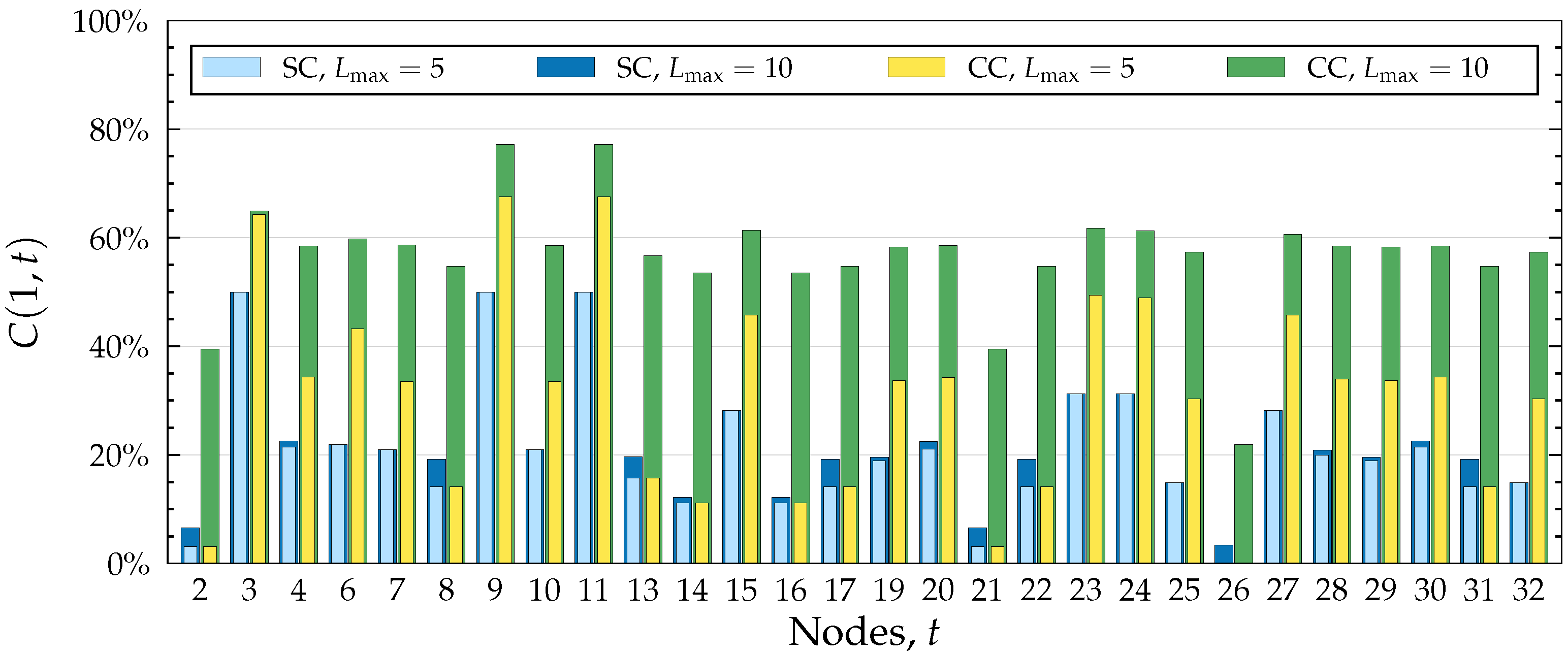
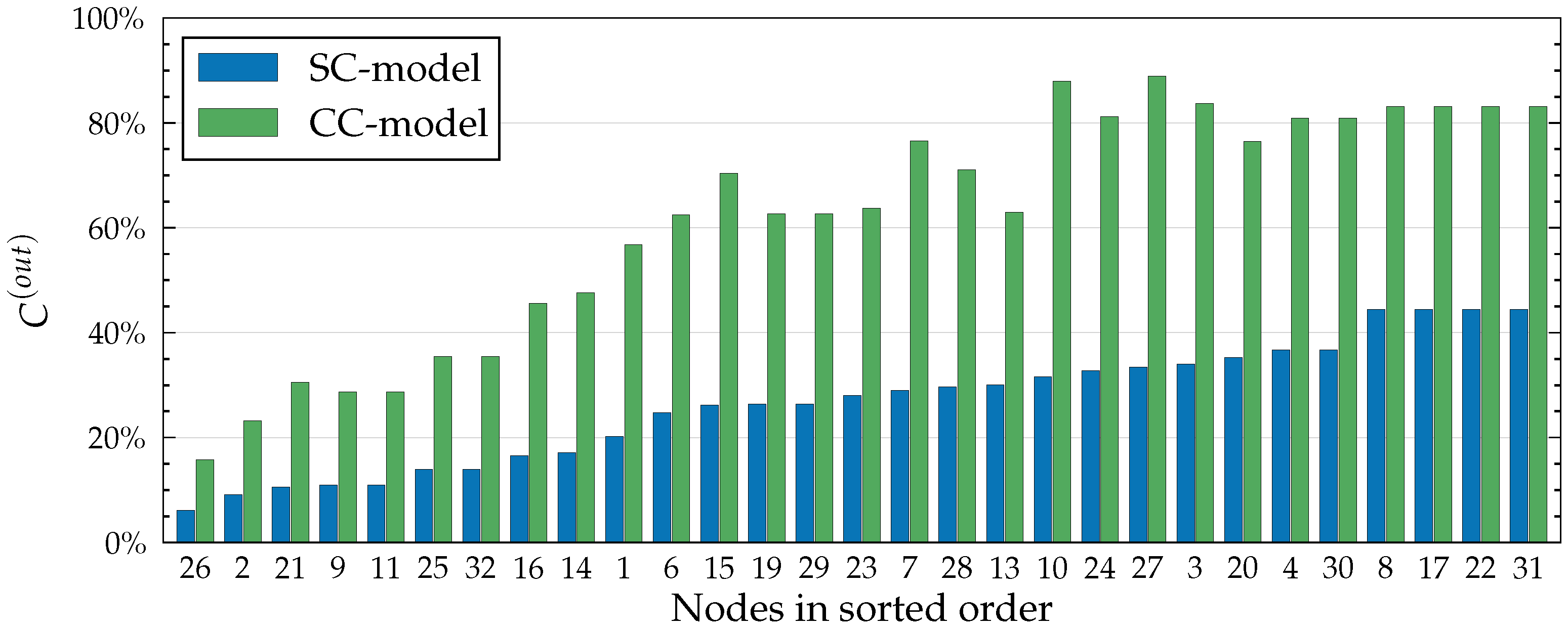
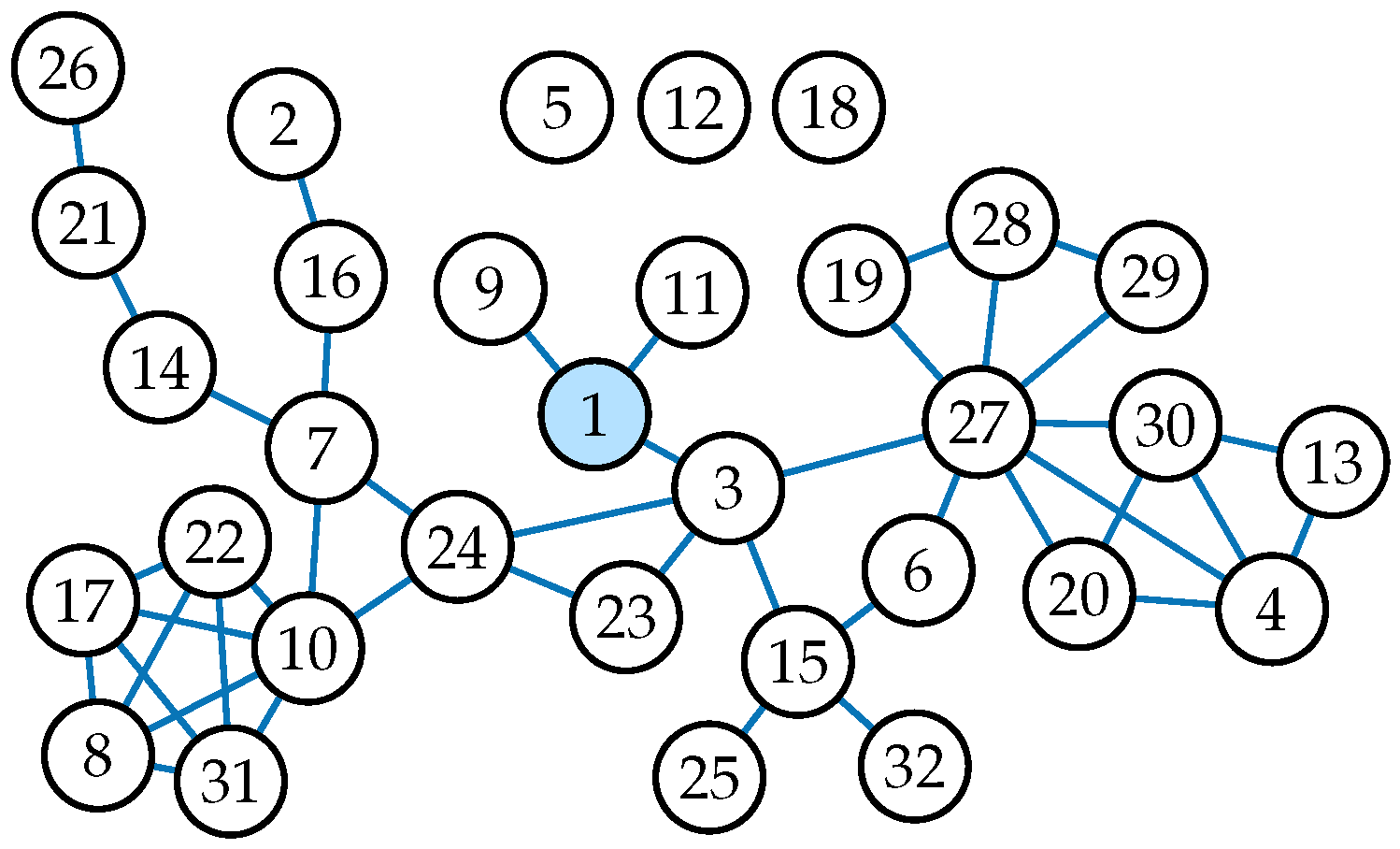
Figure 3, Figure 4 and Figure 5 illustrate different applications of our model, influence spreading probabilities, out-centrality and betweenness centrality, respectively. Notice that as centrality values are calculated from the influence spreading probabilities, betweenness centrality values are calculated from centrality values. These measures, thus, form layers of abstractions on top of each other. The depicted values are calculated in the Dutch student network (see Figure 6) with all edge weights set to , i.e., for all , where E denotes the edge set of the graph.
Figure 3 depicts probabilities of spreading from node 1 to all other nodes. It includes a comparison between two values of , the maximum number of edges allowed on a path. An important observation to make is that spreading stops at the target node, even in the CC model which otherwise allows breakthrough infections. By the path combination formula (Equation (3)), the combined probability of two paths such that one is a prefix of the other is simply the probability of the shorter path. It follows that any path which visits the target node more than once will not increase the final probability. This is visible in Figure 3 where the probability of spreading to node 3 in the CC model is noticeably smaller than to nodes 9 or 11, even though the neighbourhood of node 3 contains much more paths. This behaviour is logical when we recall that our model calculates the probability of influence spreading from one node to another; that is to say, we are not interested in the probability of being influenced more than once.
The CC model considers a set of paths that is a superset of the paths that the SC model considers. This is because all self-avoiding (SC) paths are also part of the CC model. For this reason, out-centrality values are always at least as large in the CC model (see Figure 4). Differences in out-centrality values reflect the network structure in the local neighbourhood of each node. For example, in Figure 4, node 10 has a larger CC out-centrality than node 24, while node 24 has a larger SC out-centrality. This is related to the higher edge-density in the neighbourhood of 10, which allows for relatively more CC paths than SC paths.
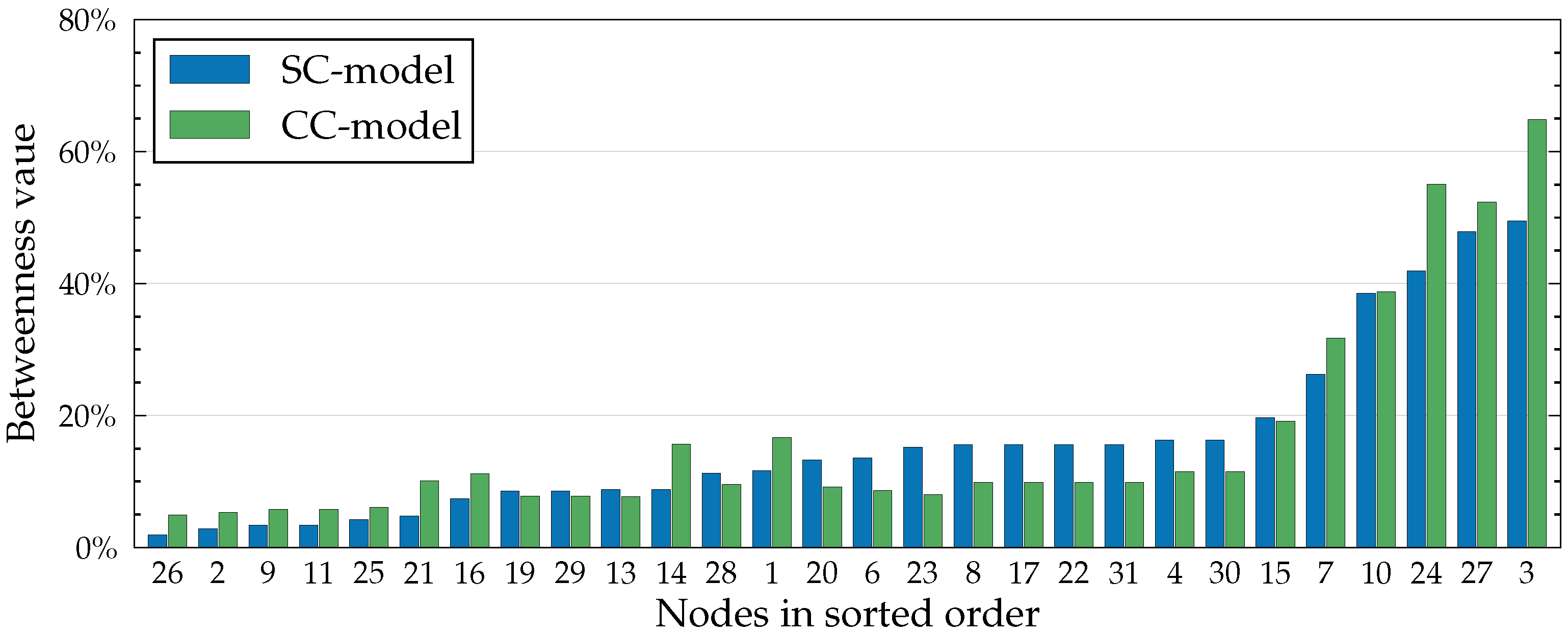
Recall from Equation (6) that betweenness is defined as the ratio of change in cohesion to the original cohesion when a node is removed from the network. In other words, betweenness corresponds to the relative importance of a node in the network. Because of this, some nodes become larger betweenness values in the SC model than in the CC model, even though the underlying centrality values are always smaller in the SC model. For example, in Figure 5, node 23 is a clear example of this. From Figure 6, we see that node 23, while being an important mediator in the network, is not part of many cycles, which decreases its relative importance in the CC model.
4. Discussion
Diffusion in various kinds of real-world situations often requires its own type of model. Some phenomena can be modelled effectively with analytical models, while others cannot. Sometimes simulation is the only option if no efficient analytical model exists or has been discovered. Generally speaking, simulation of diffusion turns out to be slow, in which case analytical models—like our efficient one—should be preferred instead. Our model has many applications and a lot of possibilities for future research. For example, the model allows the use of any path length-dependent probability distribution. It is also possible to alter the edges’ probabilities based on the distance from the original spreader. Even empirical distributions could be used to model real-world phenomena.
Computation of self-avoiding spreading requires information about the current spreading path, which makes the analytical computation of influence spreading using self-avoiding models inefficient. However, using simulation, asymptotically more efficient models with the same accuracy have been previously developed [5]. Furthermore, there are some features which naturally lead to simulation. One of them is controlling breakthrough infections. If we want to, say, assign a probability for breakthrough infections, we need to store the state of each node to determine whether a node is already infected or not. A large amount of possible states makes any analytical model inefficient, and we are, thus, left with simulation models.
Unlike other diffusion models, our model has a clear physical interpretation as all measures are based on influence spreading probabilities. The pairwise spreading probabilities found in the influence spreading matrix naturally lead to the interpretation of the centrality measures from Equations (4) and (5) as expected values. These can, in turn, be used as a measure in Equation (6) for calculating betweenness centrality values. A probability-based approach also allows the use of well-known probability distributions, like the Poisson distribution in Equation (1).
Our path-based approach has several unique characteristics not found in other models. To start with, it allows us to efficiently limit the spreading to the neighbourhood of a node. This makes it possible to study and compare a node’s importance in different-sized communities surrounding it. Furthermore, our model takes all possible paths into account, which means that the complete structure of the network is reflected in the spreading probabilities, and by extension in the betweenness centrality values from Equation (6). This is in contrast to the more common geodesic-based centrality [27], which only takes the shortest paths between pairs of nodes into account. Moreover, if we increase enough, the resulting probabilities describe the global structure of the network. In summary, the model scales naturally from analysing the local structure of a network to analysing its global structure.
5. Conclusions
Analysing large networks and, at the same time, utilising accurate methods and algorithms to obtain reliable and sufficiently detailed results are two opposing requirements in selecting the research methods and the size of the research material. This dilemma is present both in scientific and business fields, where researchers and data scientists extract information and knowledge useful for making new discoveries and supporting decision-making processes.
In this study, we have presented two programming models and their respective pseudo-algorithms for analysing complex networks, particularly in the field of social networks and social media. Both models describe the structure of a network on a detailed level. The two algorithms are based on the same influence spreading model describing how paths should be merged in order to calculate spreading probabilities between any pair of nodes. The model has multiple unique and original features, and while it is itself too inefficient for most of the real-world network sizes, both presented algorithms scale well even to large networks.
The two approaches differ in their application area in describing different processes on social networks. The efficient algorithm (Algorithm 2) is designed for analysing a wide range of complex contagion processes on social networks. In this study, we have concluded that most of the real-world processes are variants of complex contagion processes or, at least, are dominated by such social influence mechanisms.
The second algorithm (Algorithm 3) can be used for analysing simple contagion processes on social networks. Technically, the efficient algorithm allows circular and repeated events on the network structure, whereas Algorithm 3 has a strict constraining rule of allowing only self-avoiding paths during the spreading process. Both approaches have their advantages, and both are needed for modelling different kinds of spreading mechanisms.
We have discussed how our two proposed algorithms are dualistic approaches in the sense that the efficient algorithm enables an unrestricted social influence mechanism between actors on social networks whereas the less efficient algorithm has limitations on the analysed network sizes within a reasonable computing time. However, in these problems, high-performance computers and parallel computing can be used to analyse even larger networks to obtain valuable information and knowledge. In fact, both algorithms of this study are easily adapted to a parallel computing model, making them scalable for processing larger and larger networks when the amount of computation units is increased.
The main contributions of this study are the two pseudo-algorithms for complex and simple contagion processes. We have demonstrated that both of the proposed models are needed for describing influence and information spreading on social networks. We have also presented multiple applications with physical interpretations. Interesting discoveries on the given network can be made when examining the results of the presented applications and comparing the results of the two algorithms.
Author Contributions
Conceptualisation, V.K. and H.A.; methodology, V.K. and H.A.; validation, V.K., H.A. and M.I.; formal analysis, V.K.; visualisation, H.A.; data curation, H.A.; writing—original draft preparation, H.A. and V.K.; writing—review and editing, V.K., H.A., K.K.K. and M.I.; supervision, V.K.; project administration, V.K. Based on earlier software implementations, the formal representations of the Algorithms 2 and 3 have been created by H.A. All authors have read and agreed to the published version of the manuscript.
Funding
This research received no external funding. The APC was funded by Aalto University.
Institutional Review Board Statement
Not applicable.
Informed Consent Statement
Not applicable.
Data Availability Statement
Not applicable.
Acknowledgments
Conflicts of Interest
The authors declare no conflict of interest.
Abbreviations
The following abbreviations are used in this article:
| CC | Complex Contagion |
| SC | Simple Contagion |
| LCP | Longest Common Prefix |
| DFS | Depth-first Search |
References
- Barabási, A.-L.; Pósfai, M. Network Science; Cambridge University Press: Cambridge, UK, 2016. [Google Scholar]
- Newman, M.E.J. Networks: An Introduction; Oxford University Press: Oxford, UK; New York, NY, USA, 2018. [Google Scholar]
- Boccaletti, S.; Latora, V.; Moreno, Y.; Chavez, M.; Hwang, D.U. Complex networks: Structure and dynamics. Phys. Rep. 2006, 424, 175–308. [Google Scholar] [CrossRef]
- Tian, Y.; Lambiotte, R. Unifying Diffusion Models on Networks and Their Influence Maximisation. CoRR 2021, abs/2112.01465. [Google Scholar] [CrossRef]
- Luo, Z. Network Research: Exploration of Centrality Measures and Network Flows Using Simulation Studies. Available online: essay.utwente.nl/76847/1/LuoMAEEMCS.pdf (accessed on 29 June 2022).
- Kuikka, V. Influence spreading model used to analyse social networks and detect sub-communities. Comput. Soc. Netw. 2018, 5, 12. [Google Scholar] [CrossRef] [PubMed] [Green Version]
- Kuikka, V. Modelling epidemic spreading in structured organisations. Phys. A Stat. Mech. Its Appl. 2022, 592, 126875. [Google Scholar] [CrossRef]
- Codd, E.F. A Relational Model of Data for Large Shared Data Banks. Commun. ACM 1970, 13, 377–387. [Google Scholar] [CrossRef]
- Rogers, E.M. Diffusion of Innovations, 5th ed.; Free Press: New York, NY, USA, 2003; p. 576. [Google Scholar]
- Peralta, A.F.; Kertész, J.; Iñiguez, G. Opinion Dynamics in Social Networks: From Models to Data. Available online: https://arxiv.org/pdf/2201.01322 (accessed on 29 June 2022).
- Centola, D. How Behavior Spreads: The Science of Complex Contagions; Princeton University Press: Princeton, NJ, USA, 2018. [Google Scholar]
- Kirkley, A.; Cantwell, G.T.; Newman, M.E.J. Belief propagation for networks with loops. Sci. Adv. 2021, 7, eabf1211. [Google Scholar] [CrossRef] [PubMed]
- Centola, D.; Macy, M. Complex Contagions and the Weakness of Long Ties. Am. J. Sociol. 2007, 113, 702–734. [Google Scholar] [CrossRef] [Green Version]
- Min, B.; Miguel, M. Competing contagion processes: Complex contagion triggered by simple contagion. Sci. Rep. 2018, 8, 10422. [Google Scholar] [CrossRef] [PubMed]
- Ijäs, M.; Levijoki, J.; Kuikka, V. Scalable Algorithm for Computing Influence Spreading Probabilities in Social Networks. In Proceedings of the 5th European Conference on Social Media (ECSM 2018), Limerick, Ireland, 21–22 June 2018; pp. 76–84. [Google Scholar]
- Kempe, D.; Kleinberg, J.; Tardos, É. Maximizing the Spread of Influence through a Social Network. In Proceedings of the Ninth ACM SIGKDD International Conference on Knowledge Discovery and Data Mining, KDD’03, Washington, DC, USA, 24–27 August 2003; Association for Computing Machinery: New York, NY, USA, 2003; pp. 137–146. [Google Scholar]
- Gómez, S. Centrality in networks: Finding the most important nodes. In Proceedings of the Business and Consumer Analytics: New ideas. Part III, Chapter 8; Moscato, P., de Vries, N.J., Eds.; Springer International Publishing: Cham, Switzerland, 2019; pp. 401–434. [Google Scholar]
- Borgatti, S.P. Centrality and network flow. Soc. Netw. 2005, 27, 55–71. [Google Scholar] [CrossRef]
- Katz, L. A new status index derived from sociometric analysis. Psychometrika 1953, 18, 39–43. [Google Scholar] [CrossRef]
- Bavelas, A. A mathematical model for group structures. Appl. Antropoly 1948, 7, 16–30. [Google Scholar] [CrossRef]
- Freeman, L. A set of measures of centrality based on betweenness. Sociometry 1977, 40, 35–41. [Google Scholar] [CrossRef]
- Freeman, L. Centrality in social networks conceptual clarification. Soc. Netw. 1979, 1, 215–239. [Google Scholar] [CrossRef] [Green Version]
- Fortunato, S.; Hric, D. Community detection in networks: A user guide. Phys. Rep. 2016, 659, 1–44. [Google Scholar] [CrossRef] [Green Version]
- Newman, M.E.J. Modularity and community structure in networks. Proc. Natl. Acad. Sci. USA 2006, 103, 8577–8582. [Google Scholar] [CrossRef] [PubMed] [Green Version]
- Leskovec, J.; Krevl, A. SNAP Datasets: Stanford Large Network Dataset Collection. 2014. Available online: http://snap.stanford.edu/data (accessed on 29 June 2022).
- Van de Bunt, G. Friends by Choice. An Actor-Oriented Statistical Network Model for Friendship Networks through Time. Ph.D. Thesis, University of Groningen, Groningen, The Netherlands, 1999. [Google Scholar]
- Newman, M. The Structure and Function of Complex Networks. Comput. Phys. Commun. 2003, 147, 40–45. [Google Scholar] [CrossRef]
- Kuikka, V. Influence Spreading Model Used to Community Detection in Social Networks. In Proceedings of the Complex Networks & Their Applications VI; Cherifi, C., Cherifi, H., Karsai, M., Musolesi, M., Eds.; Springer International Publishing: Cham, Switzerland, 2018; pp. 202–215. [Google Scholar]
Figure 1.
Network G, and a tree of all paths ending at node A in network G, with length at most 3, illustrating how paths are combined at their last common node. [15].
Figure 1.
Network G, and a tree of all paths ending at node A in network G, with length at most 3, illustrating how paths are combined at their last common node. [15].

Figure 2.
Relative difference in out-centrality values with different path lengths when compared to the values with in the Facebook network [25] calculated with the CC model (Algorithm 2) when for all , , and . By relative difference, we mean the largest relative difference in a node’s out-centrality value when compared to the converged value, i.e., those with . Note that the y-axis is logarithmic and that the curve is nearly linear after the start, which means that precision grows exponentially with respect to path length.

Figure 3.
Comparison of SC and CC models using spreading probabilities calculated in the Dutch Student network (see Figure 6 where node 1 is highlighted) with , , and for all . The graph depicts, for each node t, the probability of spreading from node 1 to node t. Two different path lengths are used, and .

Figure 4.
Comparison of SC and CC models using out-centrality values calculated in the Dutch Student network (see Figure 6) with , , , and for all . The out-centrality values are normalised and expressed as a percentage of all nodes. is defined for all in Equation (5).

Figure 5.
Betweenness values in the Dutch Student network (see Figure 6) with , , , and for all . Values are calculated from the influence spreading matrix according to Equation (6). Values are expressed as percentages as our definition of betweenness centrality (Equation (6)) corresponds to the relative change in cohesion (Equation (7)). The higher the percentage, the more important the node.

Figure 6.
The depicted network was constructed based on data collected by Van de Bunt [26]. It is a longitudinal friendship network among 32 Dutch students. Its small size and unique structure make it a great example network for our centrality and betweenness measures. Note that there are three unconnected nodes numbered 5, 12, and 18. They were left out of Figure 3, Figure 4 and Figure 5 as they do not provide any significant results.


Table 1.
Running times for various real-world social networks from the SNAP dataset [25] using the CC algorithm (Algorithm 2). All values were calculated with on a workstation with two Intel Xeon X5690 processors.
Table 1.
Running times for various real-world social networks from the SNAP dataset [25] using the CC algorithm (Algorithm 2). All values were calculated with on a workstation with two Intel Xeon X5690 processors.
| Network | #Nodes | #Edges | Running Time |
|---|---|---|---|
| ArXiv collaboration network (ca-GrQc) | 5242 | 14,496 | 29.2 s |
| Facebook network (ego-Facebook) | 4039 | 88,234 | 37.5 s |
| Twitter network (ego-Twitter) | 81,306 | 1,768,149 | 3.5 h |
| Google+ network (ego-Gplus) | 107,614 | 13,673,453 | 50.7 h |
Publisher’s Note: MDPI stays neutral with regard to jurisdictional claims in published maps and institutional affiliations. |
© 2022 by the authors. Licensee MDPI, Basel, Switzerland. This article is an open access article distributed under the terms and conditions of the Creative Commons Attribution (CC BY) license (https://creativecommons.org/licenses/by/4.0/).
Share and Cite
MDPI and ACS Style
Kuikka, V.; Aalto, H.; Ijäs, M.; Kaski, K.K. Efficiency of Algorithms for Computing Influence and Information Spreading on Social Networks. Algorithms 2022, 15, 262. https://doi.org/10.3390/a15080262
AMA Style
Kuikka V, Aalto H, Ijäs M, Kaski KK. Efficiency of Algorithms for Computing Influence and Information Spreading on Social Networks. Algorithms. 2022; 15(8):262. https://doi.org/10.3390/a15080262
Chicago/Turabian StyleKuikka, Vesa, Henrik Aalto, Matias Ijäs, and Kimmo K. Kaski. 2022. "Efficiency of Algorithms for Computing Influence and Information Spreading on Social Networks" Algorithms 15, no. 8: 262. https://doi.org/10.3390/a15080262
Note that from the first issue of 2016, this journal uses article numbers instead of page numbers. See further details here.