A Novel Data-Driven Magnetic Resonance Spectroscopy Signal Analysis Framework to Quantify Metabolite Concentration


1
Department of Electrical and Computer Engineering, Texas Tech University, 2500 Broadway, Lubbock, TX 79409, USA
2
Texas Tech Neuroimaging Institute, Texas Tech University, 2500 Broadway, Lubbock, TX 79409, USA
*
Author to whom correspondence should be addressed.
Algorithms 2020, 13(5), 120; https://doi.org/10.3390/a13050120
Submission received: 20 April 2020
/
Accepted: 7 May 2020
/
Published: 10 May 2020
Abstract
:Developing tools for precise quantification of brain metabolites using magnetic resonance spectroscopy (MRS) is an active area of research with broad application in non-invasive neurodegenerative disease studies. The tools are mainly developed based on black box (data-driven), or basis sets approaches. In this study, we offer a multi-stage framework that integrates data-driven and basis sets methods. We first use truncated Hankel singular value decomposition (HSVD) to decompose free induction decay (FID) signals into single tone FIDs, as the data-driven stage. Subsequently, single tone FIDs are clustered into basis sets while using initialized K-means with prior knowledge of the metabolites, as the basis set stage. The generated basis sets are fitted with the magnetic resonance (MR) spectra while using a linear constrained least square, and then the metabolite concentration is calculated. Prior to using our proposed multi-stage approach, a sequence of preprocessing blocks: water peak removal, phase correction, and baseline correction (developed in house) are used.
1. Introduction
Nuclear magnetic resonance (NMR) is an important biochemical technique for the in vitro determination of protein structure and protein-drug interaction studies [1,2], which is also being widely used in the field of in-cell NMR [3,4,5,6]. Magnetic resonance spectroscopy (MRS), which is based on NRM principles, is widely being used along with magnetic resonance imaging (MRI) to acquire detailed information about the tissue structures for medical diagnosis [7,8,9]. MRS non-invasively provides information on the brain’s metabolites concentrations, which aids the early detection of neurodegenerative diseases [10,11,12] The current developed techniques and software packages for MRS signal processing retain significant variance in the absolute metabolite quantification. Magnetic resonance (MR) spectra analysis methods can be classified as either black box (data-driven) or basis sets methods [8]. Basis set methods incorporate prior knowledge of metabolites chemical structures in both in-vivo NMR (e.g., LC ModelTM [13], TARQUIN [14]), and in-vitro NMR [15], while the black box does not incorporate prior knowledge, and are completely data-driven, such as QUEST [16].
The black box methods decompose the free induction decay (FID) signals in the time domain, and then quantify the metabolites by modeling the decomposed FID signal. Black box methods have been shown effective on sparse data, and long echo time (TE) acquisition; however, the main drawback of black box methods is impracticable results for complex data, such as short TE, due to not including prior knowledge [14,17]. The number of detected peaks in MR spectra increases using short TE scanning, which allows for the precise quantification of metabolites with short T2 relaxation time [18]; thus, the pattern complexity of some metabolites increases. Therefore, modeling the metabolites basis sets with a series of single peaks is difficult using existing black box methods.
The basis sets method match basis sets models developed in the laboratory with the MR spectra of the scanned data in the frequency domain. It has been shown that basis sets methods are more operative for complex data when compared with black box methods. However, one of the shortcomings of the basis sets methods is the existence of unknown components in the complex in vivo data, as a consequence of using basis sets that were developed in laboratory environments [8,19]. Therefore, the possibility of accuracy loss increases.
In this study we address the abovementioned issues, by the integration of the truncated HSVD and K-means clustering with centroids initialized using prior knowledge of basis sets developed in the laboratory environments. We used a phantom to generate a ground truth data to compare the accuracy of the proposed algorithm and TARQUIN. Two different brain regions of four subjects were scanned at Texas Tech Neuro-imaging Institute (TTNI) in order to provide in vivo data, allowing for a comparison of proposed approach and TARQUIN.
2. Materials and Methods
The FID signal consists of both real and imaginary terms corresponding to the x and y components of rotating magnetization, which is perpendicular to the magnetization vector in the z-axis [20]. The FID is a detectable NMR signal that generates a process known as Larmor precession [21]. The complex notation is used to represent the FID signal due to its suitability for further mathematical operations.
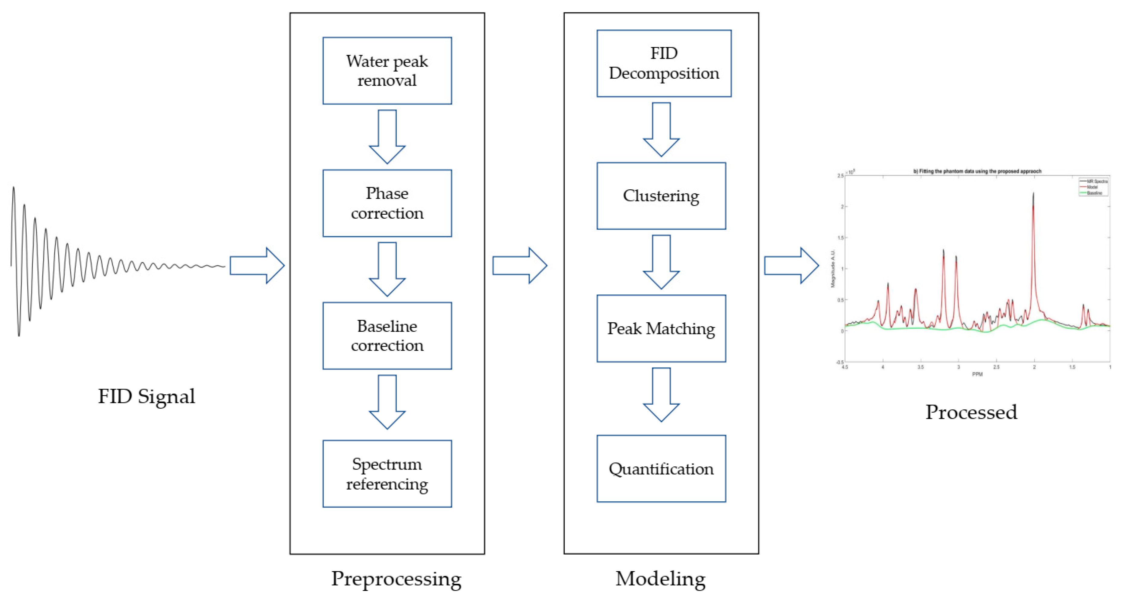
The algorithm consists of two main steps: preprocessing and modeling. Preprocessing steps include zero-filling, signal smoothing, and noise filtering [22], eddy current correction [23], water peak removal, phase correction, and baseline correction. The modeling steps include decomposition, clustering, peak matching, and quantification. Truncated HSVD is utilized to decompose the FID signal in time domain into single tone FIDs, and each tone generates a single peak in the frequency domain. K-means clustering with initialized centroids was employed to cluster the single peaks as the metabolites basis sets. The diagram of the proposed approach is shown in the Figure 1 and the details of each step are described in the following sections.
2.1. Preprocessing
In this section, we only describe those preprocessing blocks that we modified or developed. Other preprocessing blocks, such as signal smoothing, noise filteration, and eddy current correction, were applied exactly the same as described in [22,23].
2.1.1. Water Peak Removal
The water suppressed MR spectra still contains a residual water peak in the frequency range of [14]. This residual peak can be filtered out while using the maximum-phase pass-band FIR filter from [24], which is more accurate than the HSVD that is used in the TARQUIN for water peak removal. A FIR filter is a weighted sum of the most recent input values of the filter [24,25] to suppress all of the water components in the specified frequency region, while maintaining the other frequency regions with minimal distortion.
2.1.2. Phase Correction
MR spectra are not always in absorption mode, due to the misadjustment of the reference phase relative to the receiver phase detector, amplifier dead time, and phase shift from the digital filter employed to reduce noise [26]. The phase correction operation is automatically performed through application of reference [27], which combines “coarse tuning” and “fine tuning”. In the former procedure, the position of the tail ends of each peak is determined with a baseline, and then the preliminary phase spectra are obtained by minimizing the height difference between tail ends. After the coarse tuning, peaks are classified as: positive, negative, or distorted. A custom negative penalty function is generated to neglect the negative and distorted peaks. Ultimately, the phase spectra are obtained by minimizing the generated negative penalty function.
2.1.3. Baseline Correction
Separating macromolecules (MM) from the metabolites in the MR spectra, which is essential for reducing variability in the metabolite quantification, is applied through a process called baseline correction [1]. To detect the baseline and subtract it from the MR spectra, the automatic baseline correction algorithm of [7] is used. This process detects the local minima of the MR spectra to not include sharp metabolites peaks, and then iteratively generates envelopes to estimate a baseline for the MR spectra. Afterward, the estimated baseline is subtracted from the MR spectra to obtain metabolites-only MR spectra.
2.1.4. Spectrum Referencing
The inhomogeneity of the rotating magnetic field often causes a chemical shift in the MR spectra and, therefore, the selection of an identifiable reference peak to adjust the MR spectra is implemented. For in vivo 1H MRS, it is standard to define the chemical shift scale vector, ppm, as follows:
where fR represents the static magnetic field in hertz and ref is the chemical shift value at the center of the spectrum (typically 4.7 ppm for 1H MRS) [25]. For spectrum allignment, the NAA singlet peak was fixed at 2.01 ppm.
2.2. FID Decomposition
The first step to generate basis sets of data-driven modeling is decomposing the FID signal while using truncated Hankel singular value decomposition (HSVD), which decomposes the FID signal into time domain components [8,28]. The decomposition step is performed after the removal of the water peak with a time-domain FIR filter. The FID signal is described by four parameters, as depicted in Equation (2), below.
where parameters of the FID signal components are: —amplitude of a single component, —damping factor of a single component, —frequency of a single component, —sampling time, —phase of single component, and —is imaginary unit.
HSVD starts with arranging data in form of an Hankel matrix.
L and M must be chosen greater than the number of expected damped sinusoids, K. The L and M summation must be equal to N + 1, where N is number of datapoints. It is recommended to pick L and M in a way that makes SH matrix as square as possible [8].
Subsequently, the Hankel matrix is decomposed into a product of three matrices by the application of SVD.
where U and V are unitary matrixes and is a diagonal matrix, whose main diagonal elements are the singular values of . The next step is truncating into , where K is the number of sinusoids, which is assumed to be necessary to model the FID signal, and it corresponds to the number of rows of matrix and the number of columns of matrix .
To estimate eigenvalues of the state matrix corresponding to the model of (1), Equation (6), below, is formed. In (6), , and , matrices from , by omitting the first and the last row, respectively.
When the Equation (6) is solved in the least squares sense, the K eigenvalues of lead to estimates of the damping coefficients dk and frequencies fk [28].
Some of the eigenvalues are positive (driving coefficients) and others are negative (damping coefficients). Therefore, the eigenvectors that are associated with negative eigenvalues (damping coefficients) must be kept. In next step, estimates can be filled in model equation and by the least squares fit of the model (2) to the measure NMR signal. The amplitude and phase can be estimated:
By substituting (8) in (2), we have:
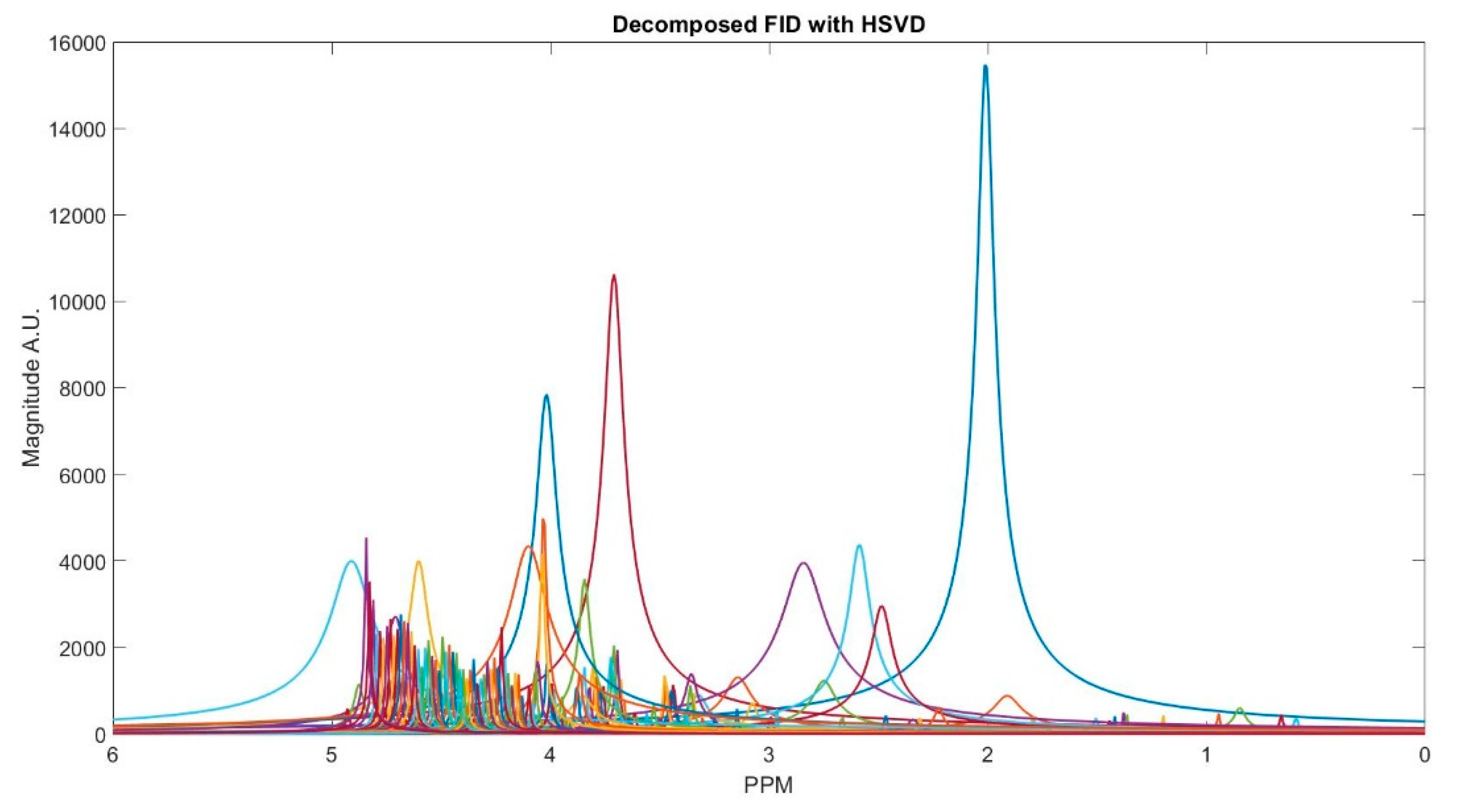
In Figure 2, we show MR spectrum of an in vivo data as an example of decomposing a FID signal while using truncated HSVD.
2.3. Clustering
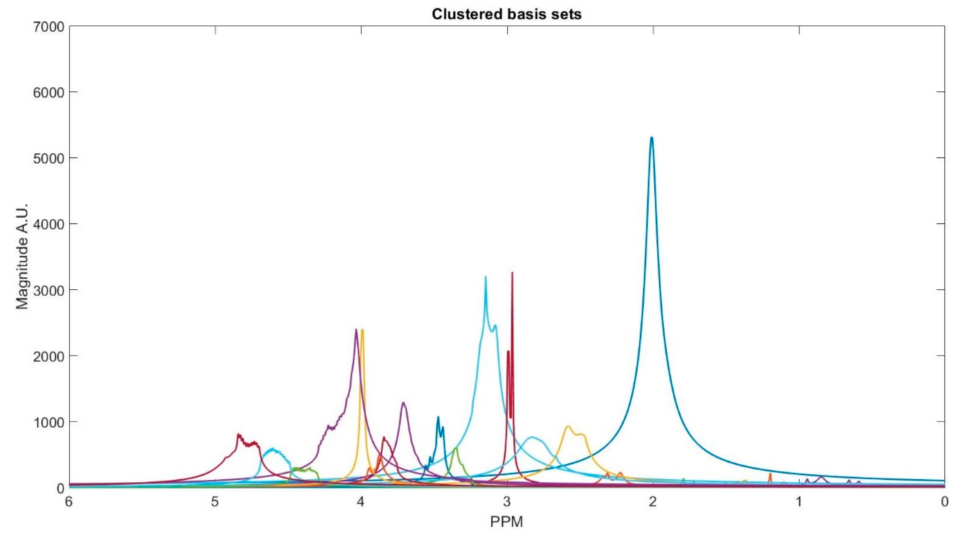
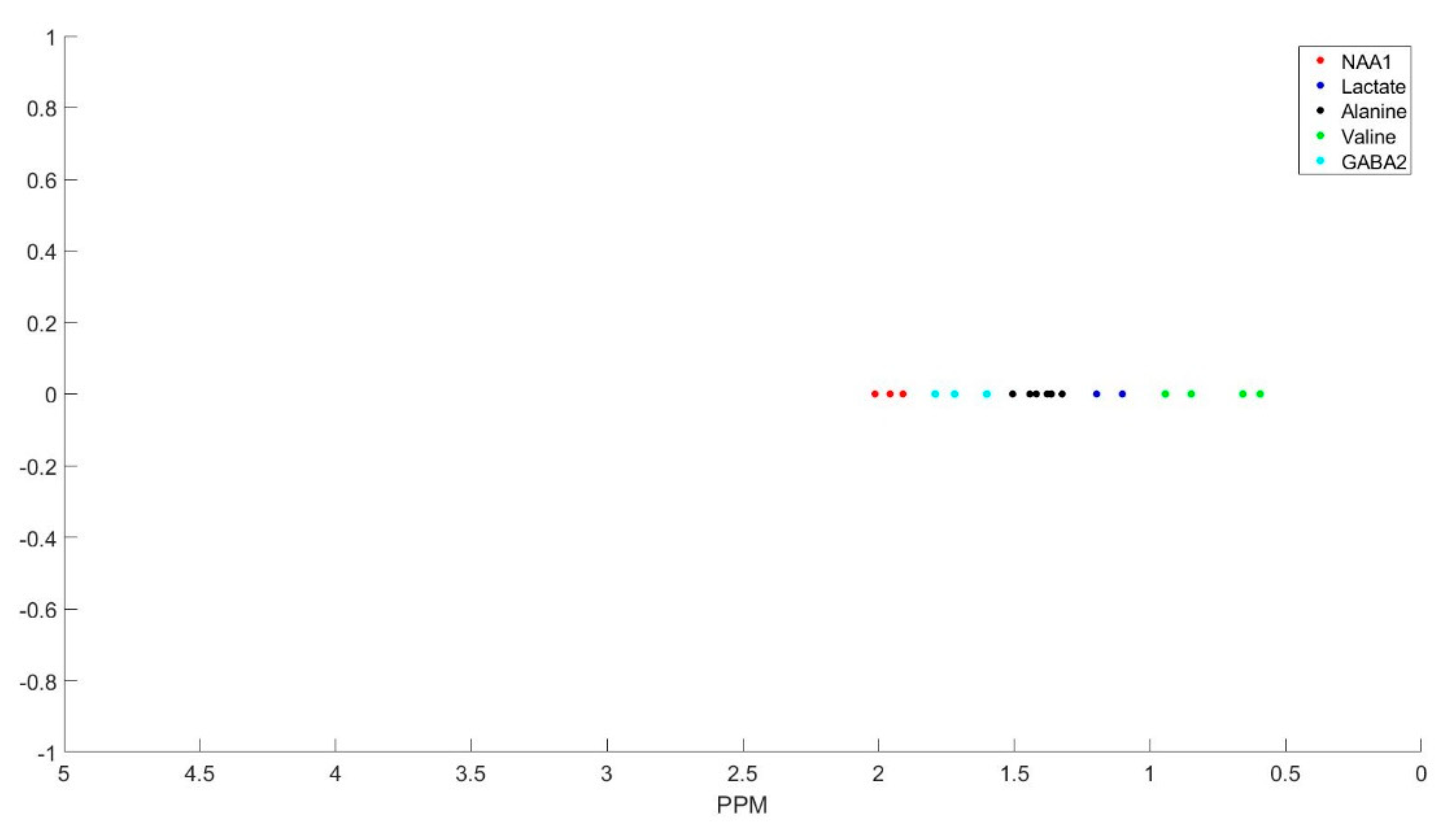
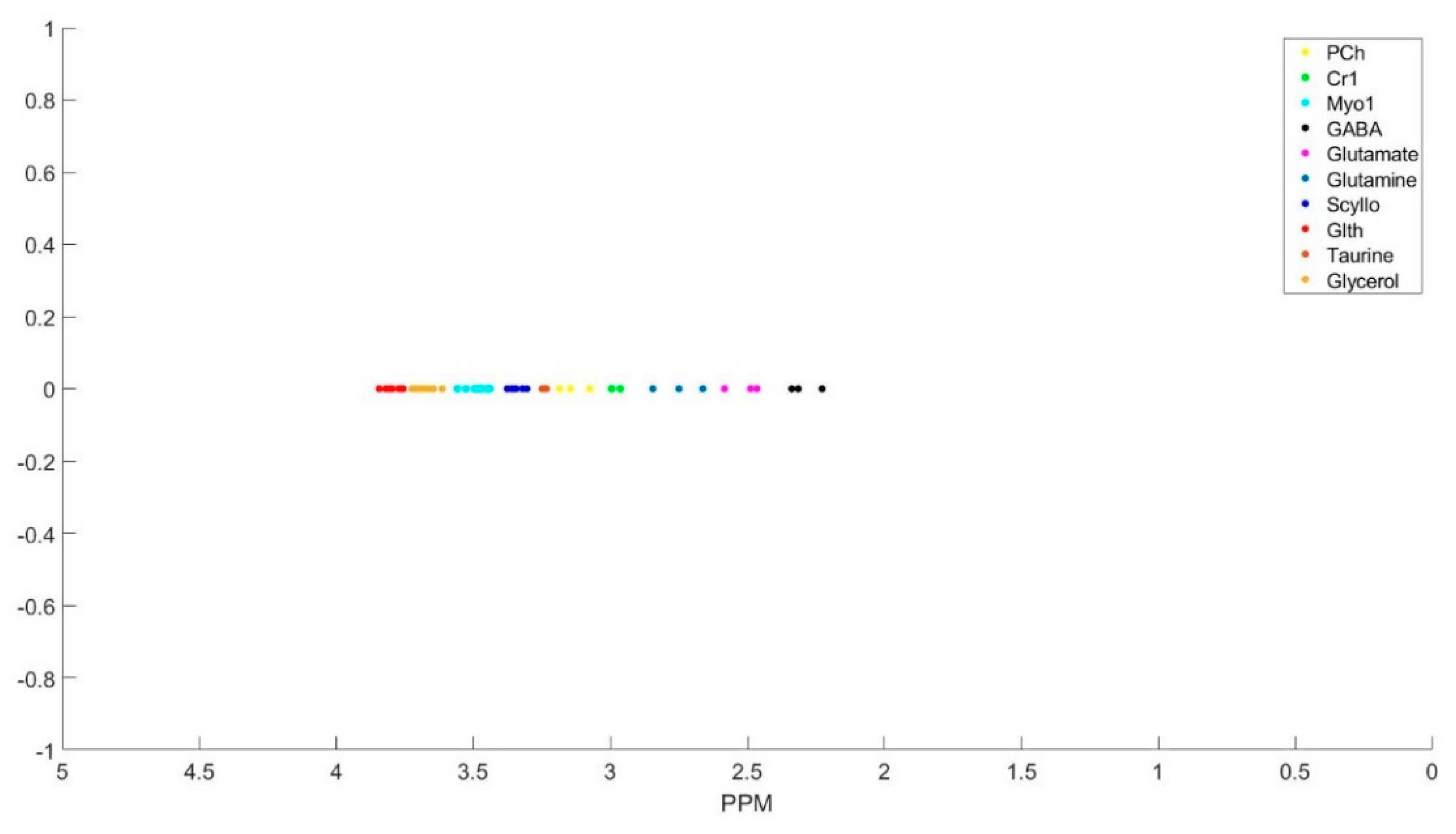
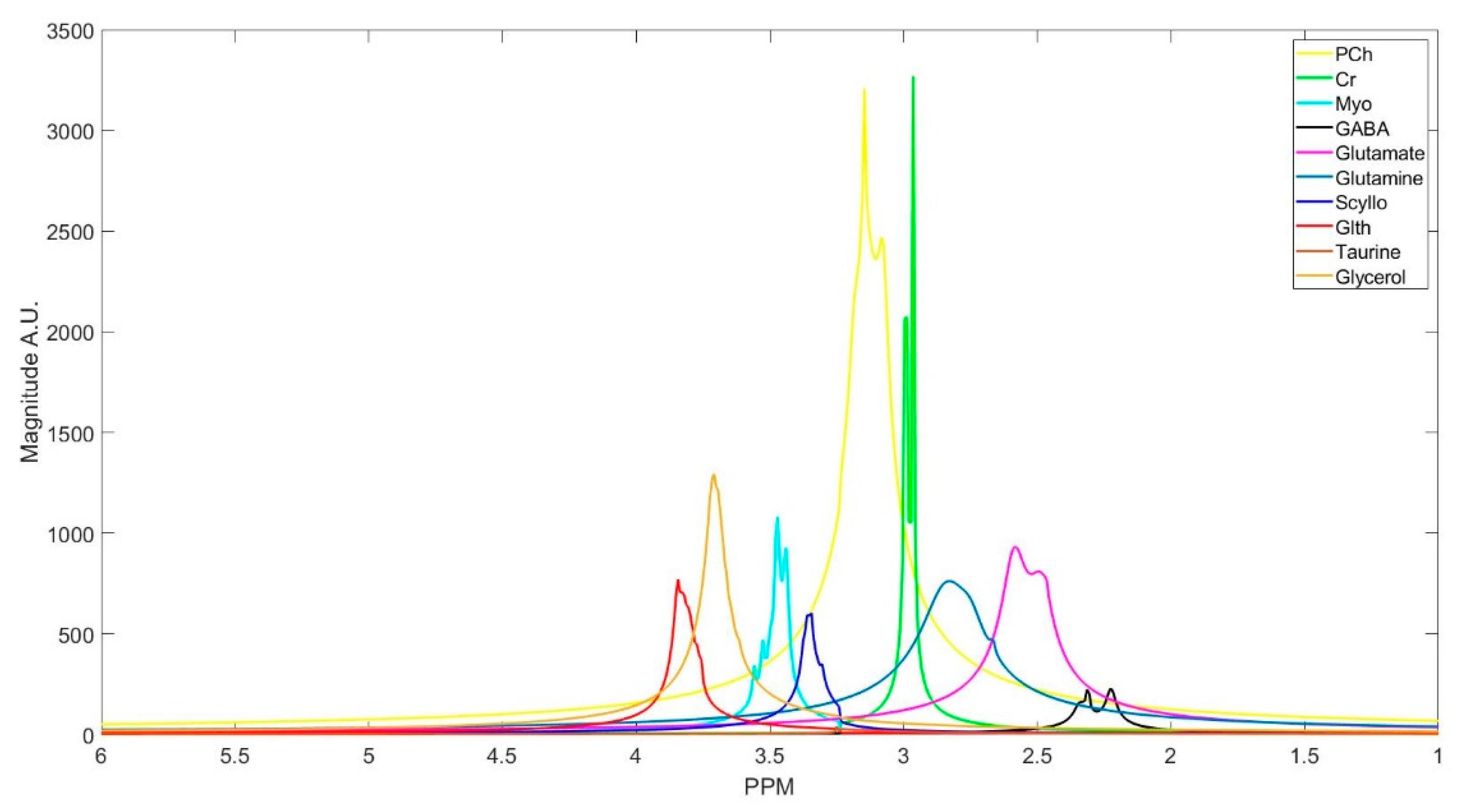
The number of decomposed FID components is larger than the number of metabolites in the FID signal. Hence, FID components need to be clustered into the number of interest metabolites. Initialized K-means is utilized to determine the cluster of components corresponding to each metabolite. K-means clustering partition number of observations; here are spectrum of the FID components, into number of clusters; here are number of metabolites, in which each component belongs to the metabolite with the nearest mean. To this end, first, the components are divided into three groups that are based on their maximum peak location in the parts per million (ppm) domain. The first group has the metabolites with peaks locations below 2.15 ppm, the second group between 2.16 and 3.85 ppm, and the third group has peaks above 3.86 ppm. Second, in each group, clusters centroids are initialized while using prior knowledge of each metabolite chemical structure, and their peak locations. Table 1 details the initialized cluster centroids, as acquired from [29]. Figure 3 shows the clustering result. The clustering process is done subject-wise, meaning that we do not learn cluster centroids from the dataset, and they are already learnt. A clustering process for one of the subjects (basis sets spectra is shown in the Figure 2) is demonstrated, step-by-step, with figures in the Appendix A.
Some of the metabolites (i.e., NAA, Creatine, Myo-inositol, and GABA) employ two cluster centroids, as shown in Table 1. Creatine, Myo-inositol, and GABA have two strong peaks that are well removed from each other and, therefore, two cluster centers for each of them were used. NAA has one large peak and one small peak. If the small peak is neglected, then the components of that peak will be picked up by other cluster centroids, and the error in calculating the metabolites concentrations of those clusters increases.
2.4. Peak Matching
The clusters are modified to address minor differences in the line shapes, frequency bins, and the peak magnitudes of the clustered components to generate the ultimate metabolites’ basis set. The linear least square was applied constrained to full width half maximum (FWHM) of each metabolite to adjust the clustered components to make the model more closely represent the observed MR spectra. Mathematically, this approach finds a θ by solving the following problem:
where, in Equation (10), and are the MR spectra and the estimate of constructed metabolite spectra, respectively. The difference between each metabolite model and the observed MR spectra is only considered over the FWHM for the peak of that metabolite. The FWHM constraint was applied to omit the data points of the MR spectra with little or no information content for the chosen metabolite. In Equation (9), is the basis set of metabolites, which is generated by the clustered components, and is the weight vector that corresponds to each specific metabolite. The basis set is not orthogonal, because metabolite peaks overlap and, thus, the solution is iterative. The process is iterative until all of the metabolites’ spectra match with the pre-processed MR spectra.
2.5. Quantification
The water signal was used as the internal reference to quantify metabolite concentrations in the volume of interest (VOI) of the tissue. The internal reference is more stable than the external reference, as it is not associated with considerable large inter-individual variability [30,31]. The internal reference spectra must be generated by the same brain VOI that generates the metabolite spectra [25,32]. Water reference is a very strong signal that can be quickly acquired, even though it must be done without water suppression in a separate scan [33]. The area under the water MR spectra is calculated and multiplied to a correction factor to calculate water intensity:
where, is the area under the water peak, TE and TR are the echo time and the repetition time, respectively, and T1w and T2w are the water relaxation times. Equation (2) was obtained from [34].
The metabolite concentrations are calculated, while using area of a peak by integrating over a fitted basis model function for that metabolite. Specifically, the intensity of a peak, p, of metabolite, m, from MRS data derived from a PRESS pulse sequence is given by:
where [m] is the concentration of metabolite, m; is the intensity of metabolite m in peak p; Nm,p is the number of hydrogens in the molecular group of m that gives rise to peak, p, K is a scale factor that takes into account the MR machine, TE and TR are the echo and repetition times of the PRESS sequence; and, T1m,p and T2m,p are the longitudinal and transverse relaxation times of the hydrogen in the molecular group of m that gives rise to peak, p. Hence, the absolute quantification of metabolite concentration is achievable using a water reference concentration, yielding:
where all of the water quantities are denoted by the W and the sum is over all resolvable peaks. Equations (12)–(14) are from [1,29,35].
2.6. Data Acquisition for Methodology Validation
MR spectroscopy signals from both in vitro (phantom) data and in vivo (subject) data are acquired with the Siemens 3T Skyra scanner at the TTNI by a Point RESolved Spectroscopy (PRESS) sequence. Each data scan was acquired with the following pulse sequence parameters: TE/TR = 30/2000 ms, voxel size = 2 × 2 × 2 cm3, sampling frequency for the phantom data = 2000 Hz, and in vivo data sampling frequency = 1200 Hz. For both in vitro and in vivo cases, both water suppressed, and water unsuppressed data were acquired. The phantom data contain nine different metabolites, with their concentrations are listed in Table 2. Five different MR spectra were scanned from five different regions of the same phantom.
The in vivo MRS and MRI data were collected from two different regions of four healthy volunteers. Two brain regions of each subject that are commonly affected by Alzheimer’s disease, the Inferior Precuneus (IP) and the Posterior Cingulate Cortex (PCC), were scanned [36,37]. For one of the subjects, in addition to PCC and IP, three other regions (left and right hippocampus, as well as ventral posterior cingulate gyrus) were also scanned, in order to assess water concentration variability in different brain regions of an individual.
3. Results
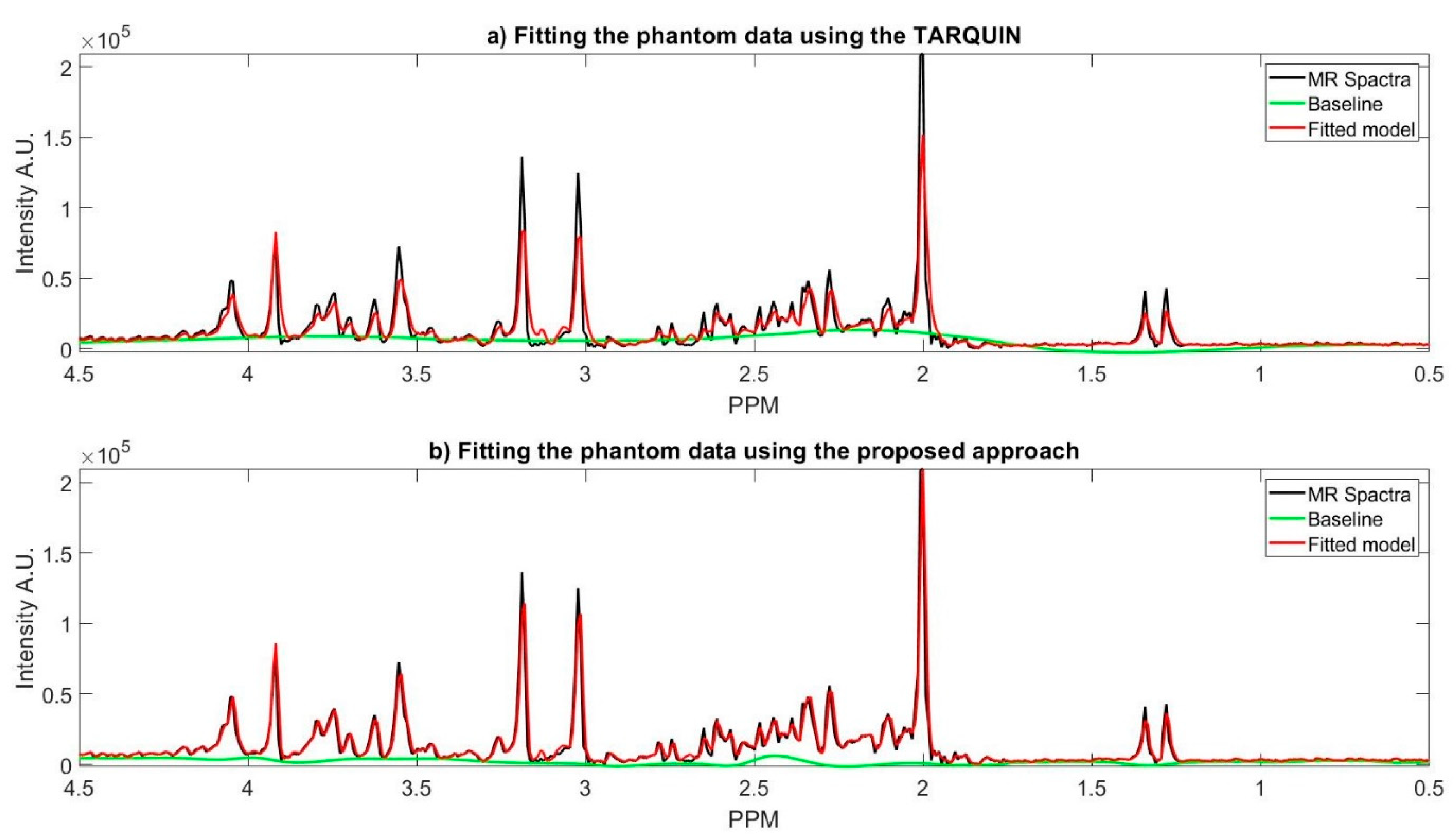
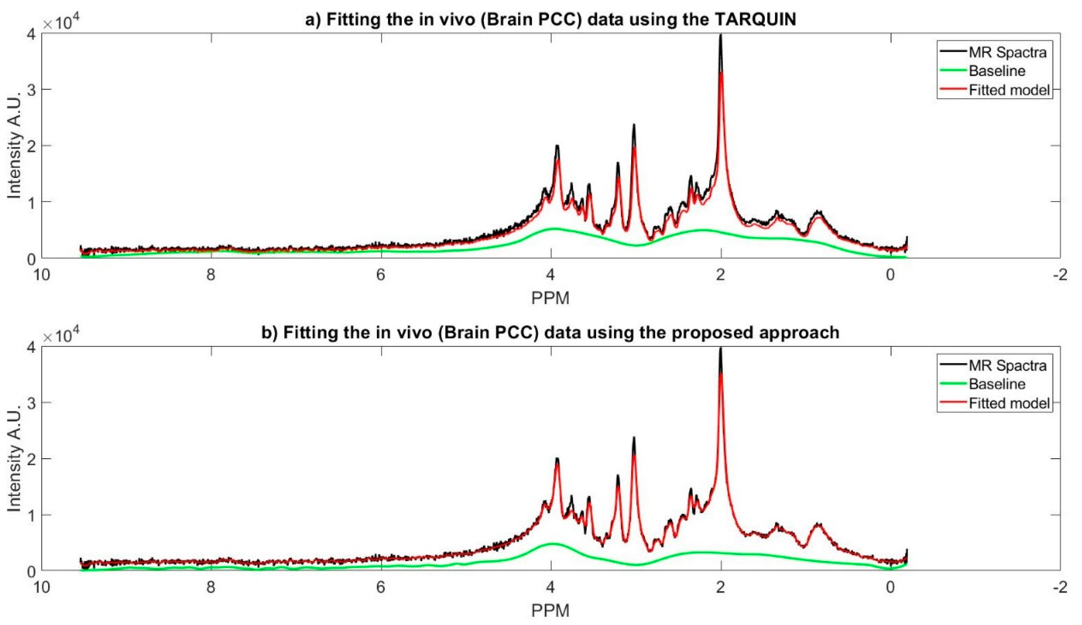
Figure 4a shows TARQUIN model fits and the baseline of the phantom data MR spectra while using a short TE PRESS sequence with a customized setting, where the reference signals are NAA, Creatine, Choline. In this customized setting, we only used the basis set of the existing metabolites of the phantom. The existing metabolites’ basis set must be selected, because TARQUIN, by default, uses basis set of 26 metabolites and macromolecules to fit the MR spectra. Therefore, if the default setting is used for fitting the non-existing metabolites, it will cause over or under estimation of existing metabolites concentration and might report some metabolites concentrations that do not exist in the phantom. Even with this modified setting, TARQUIN may not e properly stimate the existing metabolite properly. For instance, as it is shown in the Figure 4, TARQUIN overestimates the baseline in two regions, where the peak of Glutathione and Glutamate is located. Thus, this overestimation leads to mis-quantification of these two metabolites. On the other hand, the creatine and NAA peaks are not detected properly and consequently did not match perfectly due to misalignment of their peaks with the basis sets. Therefore, NAA and Creatine are underestimated for the specific example that is provided in the Figure 4.
Figure 4b shows the fit of the proposed approach model to the phantom data and the estimated baseline. In the proposed approach, the estimated baseline is very smooth as compared to the TARQUIN estimation. In contract with TARQUIN, we model the baseline as a preprocessing step prior to model each metabolite MR spectra, while TARQUIN models the metabolite first and then considers the residual as the baseline. The subtraction of the baseline prior to modeling leads to more accurate estimation of the metabolite’s MR spectra, as is shown in the Figure 4b. The main peaks including the NAA, Creatine, Choline, and Myo-inositol are matched more accurately with the MR spectra. More specifically, TARQUIN tries to detect the metabolites using basis sets matching, and then separates the baseline and the residue from the remaining part of the MR spectra, and, therefore, the detected metabolites overlap with the estimated baseline, and they are prone to over/under quantification.
The metabolite concentrations of the phantom data in the five different regions are calculated and compared with TARQUIN; the average results along with their 95% confidence interval are provided, as shown in Table 3. The mean squared error (MSE) of each quantification method calculated using the provided ground truth of the phantom data in the Table 3. The proposed approach MSE is 0.34 while the MSE associated with the TARQUIN for the phantom data is 0.94. It is notable to mention that the proposed approach provides more accurate estimation of the six out of nine metabolites concentration.
Water signal was used as the internal reference to calculate brain metabolite concentrations [25,38,39]. Water intensities of all five different brain regions of one subject were compared to investigate the possibility of reducing the scanning time. The maximum and minimum water intensities were and in arbitrary unit, respectively. Therefore, one cannot expect to scan the water unsuppressed signal for one of the brain’s region and consider that measurement provides a constant internal reference across the whole brain. Hence, for accurate metabolite concentration calculation, one must scan both waters, suppressed and unsuppressed, for each selected voxel.
For the brain regions, (IP and PCC), metabolite concentrations were calculated while using both the proposed approach and the TARQUIN. For each metabolite average and 95% confidence interval over each region were calculated and compared. Based on our observation, TARQUIN does not calculate some of the metabolite’s concentration (e.g., glycerol, valine, taurine and ATP) and also underestimates some other metabolites (e.g., glucose, Scylla-inositol, alanine, and glutamine). In the latter case, the metabolites concentration is either zero or very close to zero. Therefore, comparing the results for those metabolites is not possible. Figure 5 represents MR spectra of the one of the subjects’ brain (PCC region), and the fitted model of the proposed approach along with the TARQUIN model.
In Table 4, a comparison between our results and TARUQIN is provided. For each metabolite mean and 95% confidence interval of its concentration over all subjects within each selected brain are shown. For those metabolites with relatively high concentration, (i.e., NAA or creatine), the confidence interval is larger, relatively. Confidence interval can be a criterion to measure the consistency of the results because no ground truth is available for an in vivo data. The confidence intervals and the means are not unalike, except for Glutamate, as shown in Table 4. The TARQUIN results for glutamate vary significantly from our approach. One possible resolution can be the GLX metabolite concentration (i.e., Glutamate, Glutathione, and Glutamine). Because TARQUIN reports a very small concentration for Glutamine for all the subjects; therefore, its concentration might be assigned under the umbrella of GLX.
Full width half maximum (FWHM) also can be considered as another comparison criterion. FWHM for metabolites should be less than 0.1 ppm [9]. This fact is considered as a peak matching criterion, such that large FWHM indicates poor peak matching. The FWHM for all of the metabolites are calculated while using both the proposed approach and TARQUIN. The average of FWHM for TARQUIN and the proposed approach are 0.0375 and 0.0404 ppm, respectively.
4. Discussion
In this paper, a new data-driven algorithm for MRS signal analysis is proposed, which decomposes the FID signal in the time domain and clusters the decomposed components in the frequency domain while using prior knowledge of the chemical structure of different metabolites within the selected voxel. Although the algorithm is generalized, we have focused on the analyzing short TE 1H MRS data, due to its popularity in clinical application of MRS. We have compared against TARQUIN, as a freely available automatic software package that is widely used in MRS signal analysis applications with better claimed accuracy than the LCModelTM.
The complexity of metabolites spectra varies according to their chemical structure. For instance, the NAA spectrum frequently contains one peak that is assumed to N-acetyl aspartate [40]. The Cr peak corresponds to superposition of creatine and phosphocreatine. The PCh spectrum is more complex, containing a contribution from phosphocholine, glycerophosphocholine, free choline, acetylcholine, phosphatidylcholine, and choline-plasminogen [29]. The myo-inositol peak includes phosphatidylinositol, inositol polyphosphatide, and inositol monophosphate [30,41]. Therefore, basis sets developed in the environment laboratories must consider all of these contributions carefully, before they can be used to model the MR spectra, through the basis sets methods of MRS signal analysis. One, reason for under/over estimation of metabolite concentration using these methods could be imperfect matching of subpeaks of the complex non-orthogonal basis sets with the corresponding metabolites in the MR spectra.
The fitted model using TARQUIN in Figure 4a shows that the NAA and Creatine peaks are not properly detected. TARQUIN estimates the model using the basis sets and then estimates the baseline, which makes the modeling of the metabolite’s MR spectra an error prone task. In agreement with some literatures including [1,10], the baseline is a major source of variability, and therefore it must be detected and corrected before the peak matching step. On the other hand, TARQUIN has a fixed number of basis sets which will be fitted to a spectrum, even if that spectrum does not contain corresponding metabolites, which is a source of error in modeling and quantification of metabolites concentration of the in vitro data. In the proposed approach, the decomposing and clustering process are performed right after the water peak removal. The clustered components are then matched with the corrected MR spectra in the frequency domain. The comparison of TARQUIN results with the phantom data ground truth shows, our approach outperforms TARQUIN in quantifying the metabolite concentration.
Several important limitations must be considered. First, the metabolites relaxation times, T1 and T2, were not measured due to limited scan time; therefore, the values from other studies were used to quantify the metabolite’s concentrations [42,43], which provides a potential source of error. Second, generally, some uncertainty exists in the parameters that were used to calculate the correction factor from the internal reference, which might cause a systematic error that must be addressed in an independent study. Third, the number of subjects and their age range were too small to investigate age-related variances in the metabolite quantification process. Fourth, the study was conducted with a 3T scanner, and using MR scanner machines with higher field strength provides signals with better quality and SNR.
5. Conclusions
In this study, a robust fully automatic data-driven approach has been proposed that incorporates prior knowledge in modeling metabolites bases sets. It decomposes FID signal in the time domain, and then clusters the decomposed components in the frequency domain. When compared with TARQUIN, the proposed method on average provides more accurate metabolites concentration of phantom data. In this work, we focused on quantification of brain’s metabolites concentration using MRS, to be utilized in our future work in an early detection of neurodegenerative diseases studies, such as Alzheimer in West Texas. Additionally, since the brain’s metabolites spectrum are in a limited range, in our future works, we will develop our algorithm that is suitable for applications covers wider range of MR spectrum.
Author Contributions
Conceptualization, O.B. and S.M.; Methodology, O.B.; Software, O.B.; Validation, O.B., B.N. and S.M.; Formal analysis, O.B.; Investigation, O.B., B.N., and S.M.; Resources, O.B., E.W., and S.M.; Data curation, O.B. and E.W.; Writing—original draft preparation, O.B., E.W., B.N., and S.M.; Writing—review and editing, O.B. and B.N.; Visualization, O.B.; Supervision, B.N.; Project administration, S.M.; Funding acquisition, S.M. and B.N. All authors have read and agreed to the published version of the manuscript.
Funding
This work has been supported by internal funding from Texas Tech University.
Acknowledgments
The authors are extremely grateful to Alex Lin of the department of Radiology at Harvard Medical School for creating the MRS phantom for the Texas Tech Neuroimaging Institute. We gratefully acknowledge many discussions, evaluations, and feedback regarding this research effort with Adineh Rezaei Bazkiaei and Reza Amani.
Conflicts of Interest
The authors declare no conflict of interest.
Appendix A
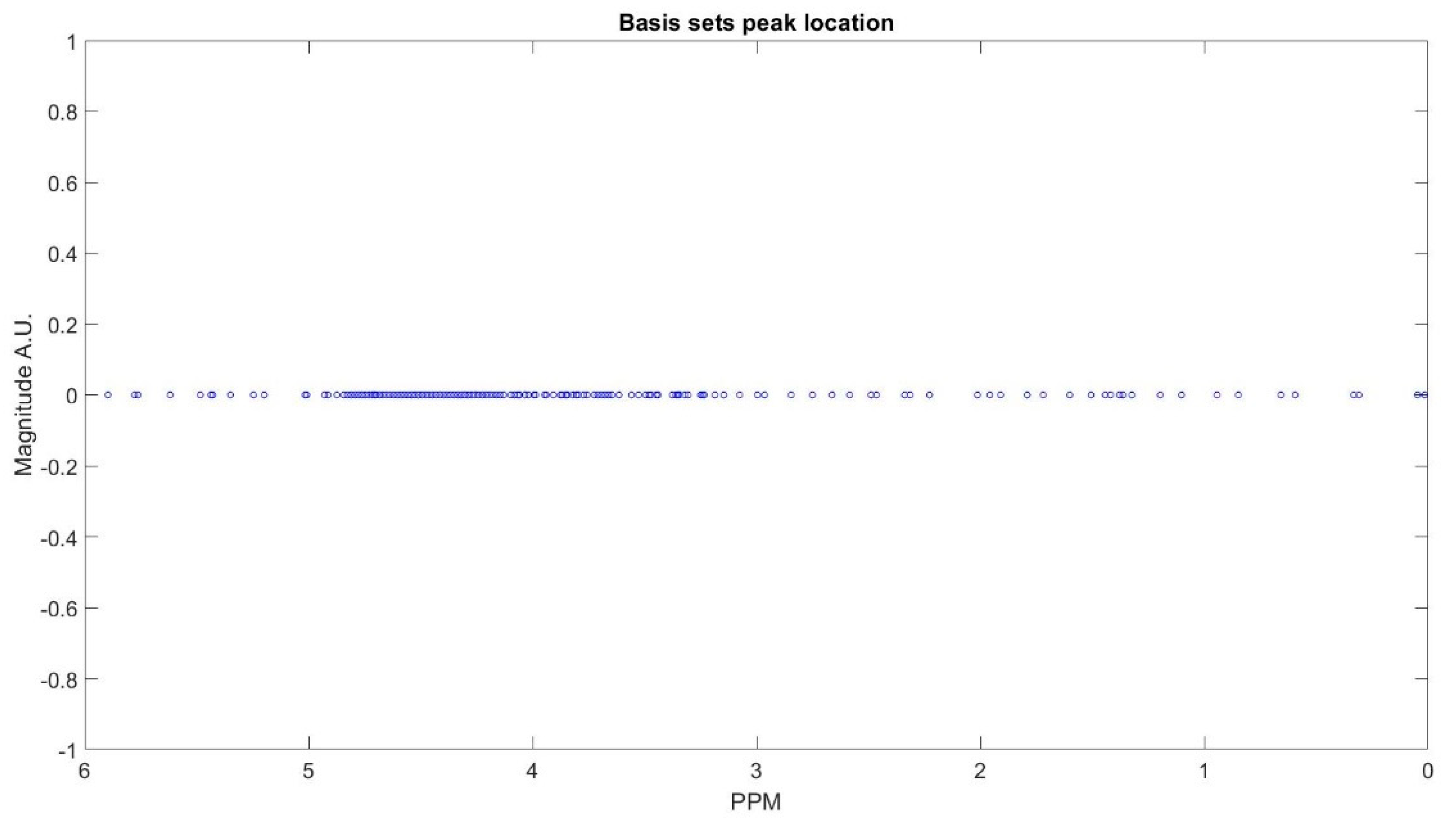
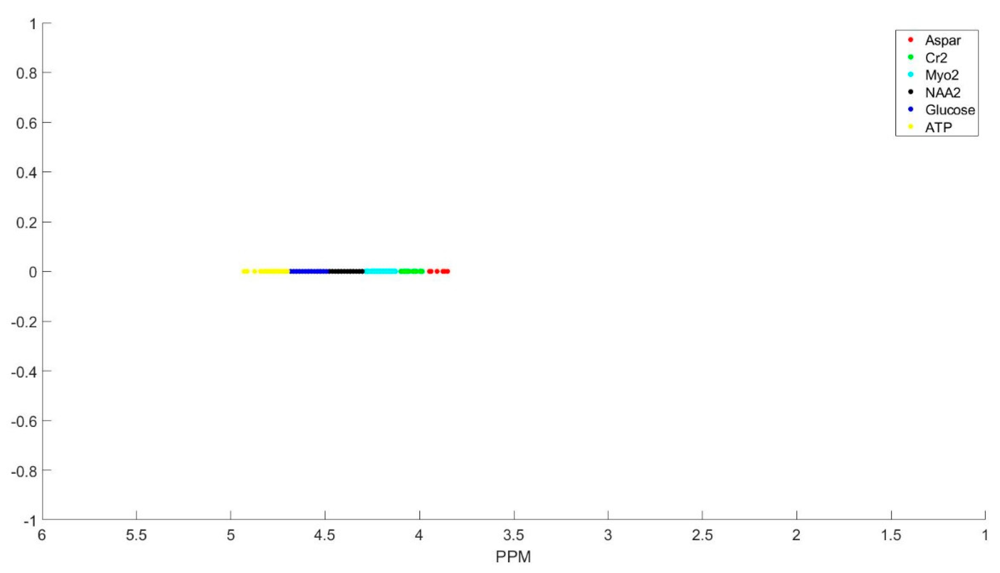
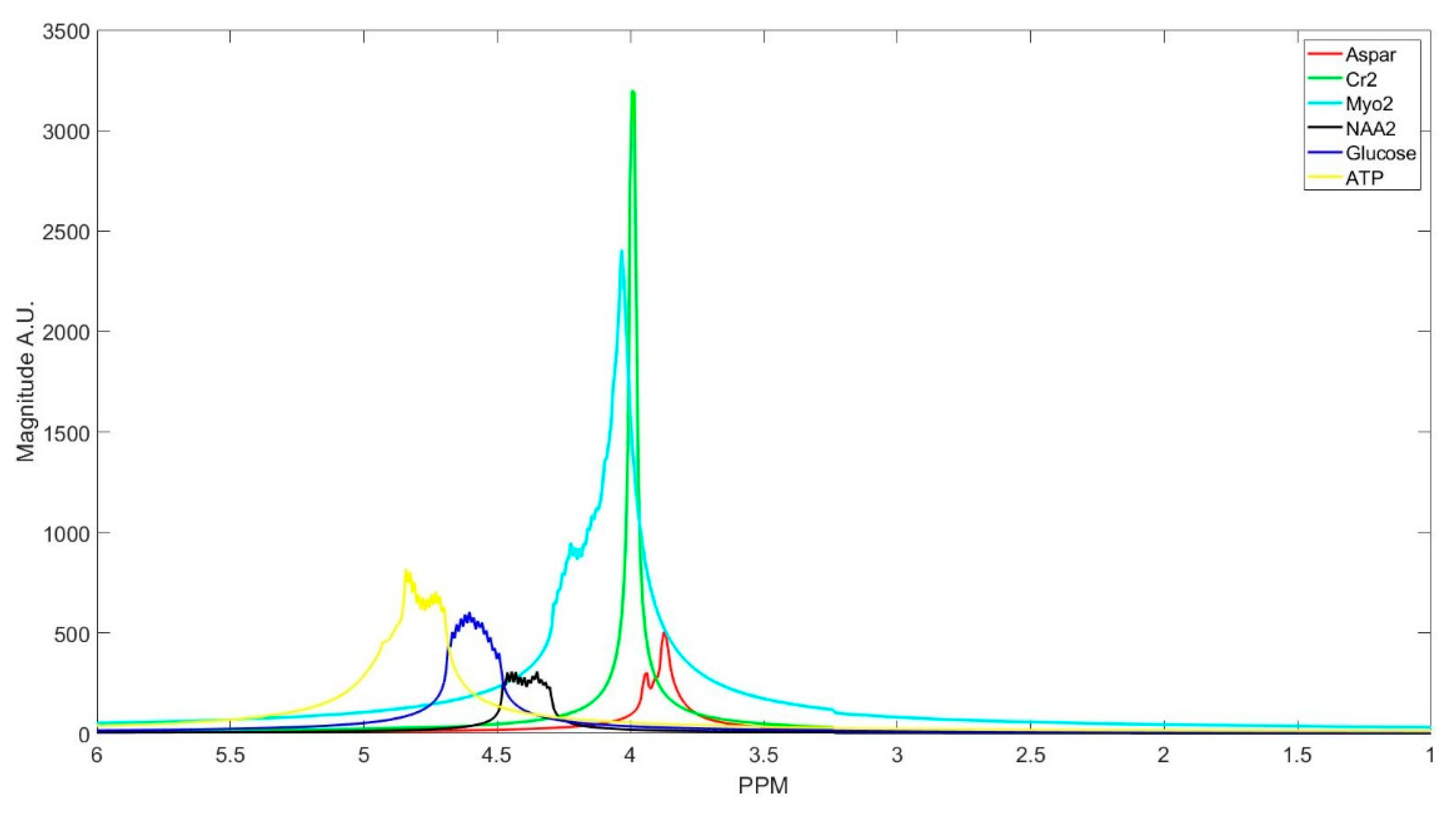
The clustering process is demonstrated with Figure A1, Figure A2, Figure A3, Figure A4, Figure A5, Figure A6 and Figure A7 step by step. First all the basis sets peak is found with their corresponding ppm as the peak locations (Figure A1). Then we select the peaks in the first group and cluster them (Figure A2), and the summation of the corresponding basis sets form each metabolite spectra (Figure A3). The same process is repeated for group 2 (Figure A4 and Figure A5) and group 3 (Figure A6 and Figure A7) of the metabolites.
Figure A1.
Peak location of basis sets of a decomposed FID signal of subject shown in the Figure 2.
Figure A1.
Peak location of basis sets of a decomposed FID signal of subject shown in the Figure 2.

Figure A2.
Metabolites listed as group 1 and their corresponding peaks.

Figure A3.
Clustered metabolites basis sets of group 1.

Figure A4.
Metabolites listed as group 2 and their corresponding peaks.

Figure A5.
Clustered metabolites basis sets of group 2.

Figure A6.
Metabolites listed as group 3 and their corresponding peaks.

Figure A7.
Clustered metabolites basis sets of group 3.

References
- Mandal, P.K. In vivo proton magnetic resonance spectroscopic signal processing for the absolute quantitation of brain metabolites. Eur. J. Radiol. 2012, 81, e653–e664. [Google Scholar] [CrossRef]
- Lambert, J.B.; Mazzola, E.P.; Ridge, C.D. Nuclear Magnetic Resonance Spectroscopy: An Introduction to Principles, Applications, and Experimental Methods; Wiley: Hoboken, NJ, USA, 2019. [Google Scholar]
- Barbieri, L.; Luchinat, E.; Banci, L. Characterization of proteins by in-cell NMR spectroscopy in cultured mammalian cells. Nat. Protoc. 2016, 11, 1101. [Google Scholar] [CrossRef] [Green Version]
- Luchinat, E.; Banci, L. A unique tool for cellular structural biology: In-cell NMR. J. Biol. Chem. 2016, 291, 3776–3784. [Google Scholar] [CrossRef] [PubMed] [Green Version]
- Amani, R.; Borcik, C.G.; Khan, N.H.; Versteeg, D.B.; Yekefallah, M.; Do, H.Q.; Coats, H.R.; Wylie, B.J. Conformational changes upon gating of KirBac1. 1 into an open-activated state revealed by solid-state NMR and functional assays. Proc. Natl. Acad. Sci. USA 2020, 117, 2938–2947. [Google Scholar] [CrossRef] [PubMed] [Green Version]
- Selenko, P.; Wagner, G. Looking into live cells with in-cell NMR spectroscopy. J. Struct. Biol. 2007, 158, 244–253. [Google Scholar] [CrossRef] [PubMed]
- Bazgir, O.; Mitra, S.; Nutter, B.; Walden, E. Fully automatic baseline correction in magnetic resonance spectroscopy. In Proceedings of the 2018 IEEE Southwest Symposium on Image Analysis and Interpretation (SSIAI), Las Vegas, NV, USA, 8–10 April 2018. [Google Scholar]
- Staniszewski, M.; Binczyk, F.; Skorupa, A.; Boguszewicz, L.; Sokol, M.; Polanska, J.; Polanski, A. Comparison of black box implementations of two algorithms of processing of NMR spectra, gaussian mixture model and singular value decomposition. BIOSIGNALS 2015. [Google Scholar] [CrossRef]
- Glenn, D.R.; Bucher, D.B.; Lee, J.; Lukin, M.D.; Park, H.; Walsworth, R.L. High-resolution magnetic resonance spectroscopy using a solid-state spin sensor. Nature 2018, 555, 351. [Google Scholar] [CrossRef] [PubMed] [Green Version]
- Poullet, J.-B.; Sima, D.M.; Van Huffel, S. MRS signal quantitation: A review of time-and frequency-domain methods. J. Magn. Reson. 2008, 195, 134–144. [Google Scholar] [CrossRef] [PubMed]
- Bartolomeo, L.A.; Wright, A.M.; Ma, R.E.; Hummer, T.A.; Francis, M.M.; Visco, A.C.; Mehdiyoun, N.F.; Bolbecker, A.R.; Hetrick, W.P.; Dydak, U.; et al. Relationship of auditory electrophysiological responses to magnetic resonance spectroscopy metabolites in early phase psychosis. Int. J. Psychophysiol. 2019, 145, 15–22. [Google Scholar] [CrossRef]
- Seo, S.E.; Tabei, F.; Park, S.J.; Askarian, B.; Kim, K.H.; Moallem, G.; Chong, J.W.; Kwon, S.O. Smartphone with optical, physical, and electrochemical nanobiosensors. J. Ind. Eng. Chem. 2019, 77, 1–11. [Google Scholar] [CrossRef]
- Provencher, S.W. Estimation of metabolite concentrations from localized in vivo proton NMR spectra. Magn. Reson. Med. 1993, 30, 672–679. [Google Scholar] [CrossRef] [PubMed]
- Wilson, M.; Reynolds, G.; Kauppinen, R.A.; Arvanitis, T.N.; Peet, A.C. A constrained least-squares approach to the automated quantitation of in vivo 1H magnetic resonance spectroscopy data. Magn. Reson. Med. 2011, 65, 1–12. [Google Scholar] [CrossRef] [PubMed]
- Reynolds, G.; Wilson, M.; Peet, A.; Arvanitis, T.N. An algorithm for the automated quantitation of metabolites in in vitro NMR signals. Magn. Reson. Med. J. Int. Soc. Magn. Reson. Med. 2006, 56, 1211–1219. [Google Scholar] [CrossRef] [PubMed]
- Ratiney, H.; Sdika, M.; Coenradie, Y.; Cavassila, S.; Ormondt, D.V.; Graveron-Demilly, D. Time-domain semi-parametric estimation based on a metabolite basis set. NMR Biomed. Int. J. Devoted Dev. Appl. Magn. Reson. Vivo 2005, 18, 1–13. [Google Scholar] [CrossRef]
- Ashbrook, S.E.; Griffin, J.M.; Johnston, K.E. Recent advances in solid-state nuclear magnetic resonance spectroscopy. Annu. Rev. Anal. Chem. 2018, 11, 485–508. [Google Scholar] [CrossRef] [Green Version]
- Mekle, R.; Mlynárik, V.; Gambarota, G.; Hergt, M.; Krueger, G.; Gruetter, R. MR spectroscopy of the human brain with enhanced signal intensity at ultrashort echo times on a clinical platform at 3T and 7T. Magn. Reson. Med. J. Int. Soc. Magn. Reson. Med. 2009, 61, 1279–1285. [Google Scholar] [CrossRef] [Green Version]
- Woods, A.J.; Bikson, M.; Chelette, K.; Dmochowski, J.; Dutta, A.; Esmaeilpour, Z.; Gebodh, N.; Nitsche, M.A.; Stagg, C. Transcranial direct current stimulation integration with magnetic resonance imaging, magnetic resonance spectroscopy, near infrared spectroscopy imaging, and electroencephalography. In Practical Guide to Transcranial Direct Current Stimulation; Springer: Berlin/Heidelberg, Germany, 2019; pp. 293–345. [Google Scholar]
- Liu, H.; Bin, J.; Dong, H.; Ge, J.; Liu, Z.; Yuan, Z.; Zhu, J.; Zhang, H. Adaptive pre-whiten filtering for the free induction decay transversal signal in weak magnetic detection. Rev. Sci. Instrum. 2019, 90, 104502. [Google Scholar] [CrossRef]
- Zhu, H.; Barker, P.B. MR spectroscopy and spectroscopic imaging of the brain. In Magnetic Resonance Neuroimaging; Springer: Berlin/Heidelberg, Germany, 2011; pp. 203–226. [Google Scholar]
- Savitzky, A.; Golay, M.J. Smoothing and differentiation of data by simplified least squares procedures. Anal. Chem. 1964, 36, 1627–1639. [Google Scholar] [CrossRef]
- De Graaf, R.A. In Vivo NMR Spectroscopy: Principles and Techniques; John Wiley & Sons: Hoboken, NJ, USA, 2013. [Google Scholar]
- Poullet, J.B.; Sima, D.M.; Simonetti, A.W.; De Neuter, B.; Vanhamme, L.; Lemmerling, P.; Van Huffel, S. An automated quantitation of short echo time MRS spectra in an open source software environment: AQSES. Nmr Biomed. Int. J. Devoted Dev. Appl. Magn. Reson. Vivo 2007, 20, 493–504. [Google Scholar] [CrossRef]
- Experts’ Working Group on Advanced Single Voxel 1H, MRS; Öz, G.; Deelchand, D.K.; Wijnen, J.P.; Mlynárik, V.; Xin, L.; Mekle, R.; Noeske, R.; Scheenen, T.W.J.; Tkáč, I. Advanced single voxel 1H magnetic resonance spectroscopy techniques in humans: Experts’ consensus recommendations. NMR Biomed. 2020. [Google Scholar] [CrossRef]
- Staniszewski, M.; Skorupa, A.; Boguszewicz, L.; Sokol, M.; Polanski, A. Preprocessing methods in nuclear magnetic resonance spectroscopy. In Information Technologies in Medicine; Springer: Berlin/Heidelberg, Germany, 2016; pp. 341–352. [Google Scholar]
- Bao, Q.; Feng, J.; Chen, L.; Chen, F.; Liu, Z.; Jiang, B.; Liu, C. A robust automatic phase correction method for signal dense spectra. J. Magn. Reson. 2013, 234, 82–89. [Google Scholar] [CrossRef] [PubMed]
- Lupu, M.; Todor, D. A singular value decomposition based algorithm for multicomponent exponential fitting of NMR relaxation signals. Chemom. Intell. Lab. Syst. 1995, 29, 11–17. [Google Scholar] [CrossRef]
- Govindaraju, V.; Young, K.; Maudsley, A.A. Proton NMR chemical shifts and coupling constants for brain metabolites. NMR Biomed. 2000, 13, 129–153. [Google Scholar] [CrossRef]
- Minati, L.; Aquino, D.; Bruzzone, M.G.; Erbetta, A. Quantitation of normal metabolite concentrations in six brain regions by in-vivo 1H-MR spectroscopy. J. Med Phys. Assoc. Med Phys. India 2010, 35, 154. [Google Scholar]
- Barker, P.B.; Soher, B.J.; Blackband, S.J.; Chatham, J.C.; Mathews, V.P.; Bryan, R.N. Quantitation of proton NMR spectra of the human brain using tissue water as an internal concentration reference. NMR Biomed. 1993, 6, 89–94. [Google Scholar] [CrossRef]
- Soher, B.J.; Hurd, R.E.; Sailasuta, N.; Barker, P.B. Quantitation of automated single-voxel proton MRS using cerebral water as an internal reference. Magn. Reson. Med. 1996, 36, 335–339. [Google Scholar] [CrossRef]
- Alger, J.R. Quantitative proton magnetic resonance spectroscopy and spectroscopic imaging of the brain: A didactic review. Top. Magn. Reson. Imaging TMRI 2010, 21, 115. [Google Scholar] [CrossRef] [Green Version]
- Christiansen, P.; Henriksen, O.; Stubgaard, M.; Gideon, P.; Larsson, H. In vivo quantification of brain metabolites by 1H-MRS using water as an internal standard. Magn. Reson. Imaging 1993, 11, 107–118. [Google Scholar] [CrossRef]
- Drost, D.J.; Riddle, W.R.; Clarke, G.D. Proton magnetic resonance spectroscopy in the brain: Report of AAPM MR Task Group# 9. Med. Phys. 2002, 29, 2177–2197. [Google Scholar]
- Fayed, N.; Modrego, P.J.; García-Martí, G.; Sanz-Requena, R.; Marti-Bonmatí, L. Magnetic resonance spectroscopy and brain volumetry in mild cognitive impairment. A prospective study. Magn. Reson. Imaging 2017, 38, 27–32. [Google Scholar] [CrossRef] [Green Version]
- Shiino, A. Proton magnetic resonance spectroscopy for dementia. In Neuroimaging Diagnosis for Alzheimer’s Disease and Other Dementias; Springer: Berlin/Heidelberg, Germany, 2017; pp. 139–172. [Google Scholar]
- Choi, C.; Bhardwaj, P.P.; Seres, P.; Kalra, S.; Tibbo, P.G.; Coupland, N.J. Measurement of glycine in human brain by triple refocusing 1H-MRS in vivo at 3.0 T. Magn. Reson. Med. J. Int. Soc. Magn. Reson. Med. 2008, 59, 59–64. [Google Scholar] [CrossRef] [PubMed]
- Ogg, R.J.; Kingsley, P.B.; Taylor, J.S. “For in vivo localized” H NMR spectroscopy. J. Magn. Reson. Ser. B 1994, 104, 1–10. [Google Scholar] [CrossRef] [PubMed]
- Kreis, R.; Ernst, T.; Ross, B. Absolute quantitation of water and metabolites in the human brain. II. Metabolite concentrations. J. Magn. Reson. Ser. B 1993, 102, 9–19. [Google Scholar] [CrossRef]
- Michaelis, T.; Merboldt, K.; Bruhn, H.; Hänicke, W.; Frahm, J. Absolute concentrations of metabolites in the adult human brain in vivo: Quantification of localized proton MR spectra. Radiology 1993, 187, 219–227. [Google Scholar] [CrossRef]
- Wyss, P.O.; Bianchini, C.; Scheidegger, M.; Giapitzakis, I.A.; Hock, A.; Fuchs, A.; Henning, A. In vivo estimation of transverse relaxation time constant (T2) of 17 human brain metabolites at 3T. Magn. Reson. Med. 2018, 80, 452–461. [Google Scholar] [CrossRef] [PubMed]
- Mlynárik, V.; Gruber, S.; Moser, E. Proton T1 and T2 relaxation times of human brain metabolites at 3 Tesla. NMR Biomed. Int. J. Devoted Dev. Appl. Magn. Reson. Vivo 2001, 14, 325–331. [Google Scholar]
Figure 1.
Diagrammatic representation of preprocessing and modeling steps for metabolite concentration quantification using magnetic resonance spectroscopy (MRS).
Figure 1.
Diagrammatic representation of preprocessing and modeling steps for metabolite concentration quantification using magnetic resonance spectroscopy (MRS).

Figure 2.
Spectra of an in vivo free induction decay (FID) signal components decomposed with Hankel singular value decomposition (HSVD).
Figure 2.
Spectra of an in vivo free induction decay (FID) signal components decomposed with Hankel singular value decomposition (HSVD).

Figure 3.
Spectrum of the in vivo data FID signal components clustered into basis sets of the metabolites.
Figure 3.
Spectrum of the in vivo data FID signal components clustered into basis sets of the metabolites.

Figure 4.
(a) The fitting phantom data magnetic resonance (MR) spectra using the TARQUIN; (b) The phantom data MR spectra fitted using the proposed approach. For both figures the phantom MR spectra (black), the fitted model (red), and the estimated baseline (green).
Figure 4.
(a) The fitting phantom data magnetic resonance (MR) spectra using the TARQUIN; (b) The phantom data MR spectra fitted using the proposed approach. For both figures the phantom MR spectra (black), the fitted model (red), and the estimated baseline (green).

Figure 5.
(a) The fitting in vivo data MR spectra using the TARQUIN; (b) the in vivo data MR spectra fitted using the proposed approach. For both figures, the phantom MR spectra (black), the fitted model (red), and the estimated baseline (green).
Figure 5.
(a) The fitting in vivo data MR spectra using the TARQUIN; (b) the in vivo data MR spectra fitted using the proposed approach. For both figures, the phantom MR spectra (black), the fitted model (red), and the estimated baseline (green).


Table 1.
Cluster centroids used for initializing K-means.
| Group 1 | Group 2 | Group 3 | |||
|---|---|---|---|---|---|
| Metabolite | Cluster Centroid | Metabolite | Cluster Centroid | Metabolite | Cluster Centroid |
| NAA 1st | 2.01 | Choline | 3.18 | Aspartate | 3.86 |
| Lactate | 1.10 | Creatine 1st | 3.02 | Creatine 2nd | 3.90 |
| Alanine | 1.46 | Myo-inositol 1st | 3.52 | Myo-inositol 2nd | 4.05 |
| Valine | 0.97 | Gaba 1st | 2.36 | NAA 2nd | 4.38 |
| Gaba 2nd | 1.85 | Glutamate | 2.51 | Glucose | 4.63 |
| Glutamine | 2.40 | ATP | 5.00 | ||
| Scyllo-inositol | 3.34 | ||||
| Glutathione | 3.75 | ||||
| Taurine | 3.28 | ||||
| Glycerol | 3.60 | ||||
Table 2.
Phantom data metabolites concentration.
| Metabolites | Concentration (mM/L) |
|---|---|
| NAA | 12.5 |
| Creatine | 10.0 |
| Choline | 3.0 |
| Myo-inositol | 7.5 |
| Lactate | 5.0 |
| GABA | 3.0 |
| Glutathione | 5.0 |
| Glutamate | 12.5 |
| Glutamine | 6.0 |
Table 3.
Mean and 95% confidence interval of the phantom’s metabolite concentration quantified by the proposed approach and the TARQUIN.
Table 3.
Mean and 95% confidence interval of the phantom’s metabolite concentration quantified by the proposed approach and the TARQUIN.
| Metabolite | Concentration (Proposed) | Concentration (TARQUIN) | Ground Truth |
|---|---|---|---|
| NAA | 12.65 | 11.73 | 12.5 |
| Creatine | 10.08 | 9.32 | 10.0 |
| Choline | 2.79 | 2.94 | 3.0 |
| Myo-inositol | 7.56 | 8.13 | 7.5 |
| GABA | 3.00 | 2.40 | 3.0 |
| Lactate | 4.66 | 2.81 | 5.0 |
| Glutamate | 12.8 | 13.64 | 12.5 |
| Glutathione | 3.78 | 4.71 | 5.0 |
| Glutamine | 4.85 | 5.27 | 6.0 |
Table 4.
A comparison between in vivo metabolite concentration calculation in two brain regions (a) Posterior Cingulate Cortex (PCC) and (b) precuneus.
Table 4.
A comparison between in vivo metabolite concentration calculation in two brain regions (a) Posterior Cingulate Cortex (PCC) and (b) precuneus.
| Metabolites | (a) PCC | (b) Precuneus | ||
|---|---|---|---|---|
| Proposed | Tarquin | Proposed | Tarquin | |
| NAA | 1.52 | 1.23 | 0.88 | 0.41 |
| Creatine | 0.56 | 0.2 | 0.56 | 0.12 |
| Choline | 0.11 | 0.3 | 0.23 | 0.17 |
| Myo-inositol | 0.5 | 0.46 | 0.32 | 0.48 |
| Gaba | 0.41 | 0.47 | 0.29 | 0.73 |
| Lactate | 0.29 | 0.03 | 0.31 | 0.37 |
| Glutamate | 0.47 | 0.76 | 0.17 | 1.5 |
| Glutathione | 0.33 | 0.16 | 0.25 | 0.13 |
| Aspartate | 3.05 | 0.33 | 0.98 | 0.41 |
© 2020 by the authors. Licensee MDPI, Basel, Switzerland. This article is an open access article distributed under the terms and conditions of the Creative Commons Attribution (CC BY) license (http://creativecommons.org/licenses/by/4.0/).
Share and Cite
MDPI and ACS Style
Bazgir, O.; Walden, E.; Nutter, B.; Mitra, S. A Novel Data-Driven Magnetic Resonance Spectroscopy Signal Analysis Framework to Quantify Metabolite Concentration. Algorithms 2020, 13, 120. https://doi.org/10.3390/a13050120
AMA Style
Bazgir O, Walden E, Nutter B, Mitra S. A Novel Data-Driven Magnetic Resonance Spectroscopy Signal Analysis Framework to Quantify Metabolite Concentration. Algorithms. 2020; 13(5):120. https://doi.org/10.3390/a13050120
Chicago/Turabian StyleBazgir, Omid, Eric Walden, Brian Nutter, and Sunanda Mitra. 2020. "A Novel Data-Driven Magnetic Resonance Spectroscopy Signal Analysis Framework to Quantify Metabolite Concentration" Algorithms 13, no. 5: 120. https://doi.org/10.3390/a13050120
Note that from the first issue of 2016, this journal uses article numbers instead of page numbers. See further details here.