The Effectiveness of Self-Sufficiency Policy: International Price Transmissions in Beef Markets


Department of Economics, Setsunan University, Osaka 572-8508, Japan
*
Author to whom correspondence should be addressed.
Sustainability 2020, 12(15), 6073; https://doi.org/10.3390/su12156073
Submission received: 24 June 2020
/
Revised: 21 July 2020
/
Accepted: 24 July 2020
/
Published: 28 July 2020
(This article belongs to the Section Economic and Business Aspects of Sustainability)
Abstract
:International beef markets have shocked regional markets in importing countries due to unexpected events such as the COVID-19 epidemic, bovine spongiform encephalopathy (BSE) and high prices for grain feed. After the global food price spikes in 2008, many national governments aimed to improve food self-sufficiency to secure food supply. However, the efficacy of food self-sufficiency policy, particularly that of meat products, is not fully understood. This paper investigates the causal nexus and estimates the degree of volatility transmissions between global and regional beef prices in 10 beef-importing nations for the period January 2006 to December 2013. Furthermore, we empirically analyze how beef self-sufficiency rates affect the correlations between global and local beef markets using a panel analysis. Our primary findings are: (1) Unidirectional causality from global to local markets was found for Georgia, the UK and the United States. Meanwhile, Japan is a large beef importer, and its price causally influences global prices; (2) We found that the interconnectivity between world and regional markets is relatively weak. Regional markets can absorb external shocks in the meat sector better than wheat because meat production is more flexible than grain production, which is heavily dependent on climatic conditions and (3) Empirical results provide strong indications that high self-sufficiency is useful in isolating local markets from global markets. The results obtained from our analysis are extremely useful for policymakers of national governments who desire to insulate domestic from international beef markets in an emergent situation.
1. Introduction
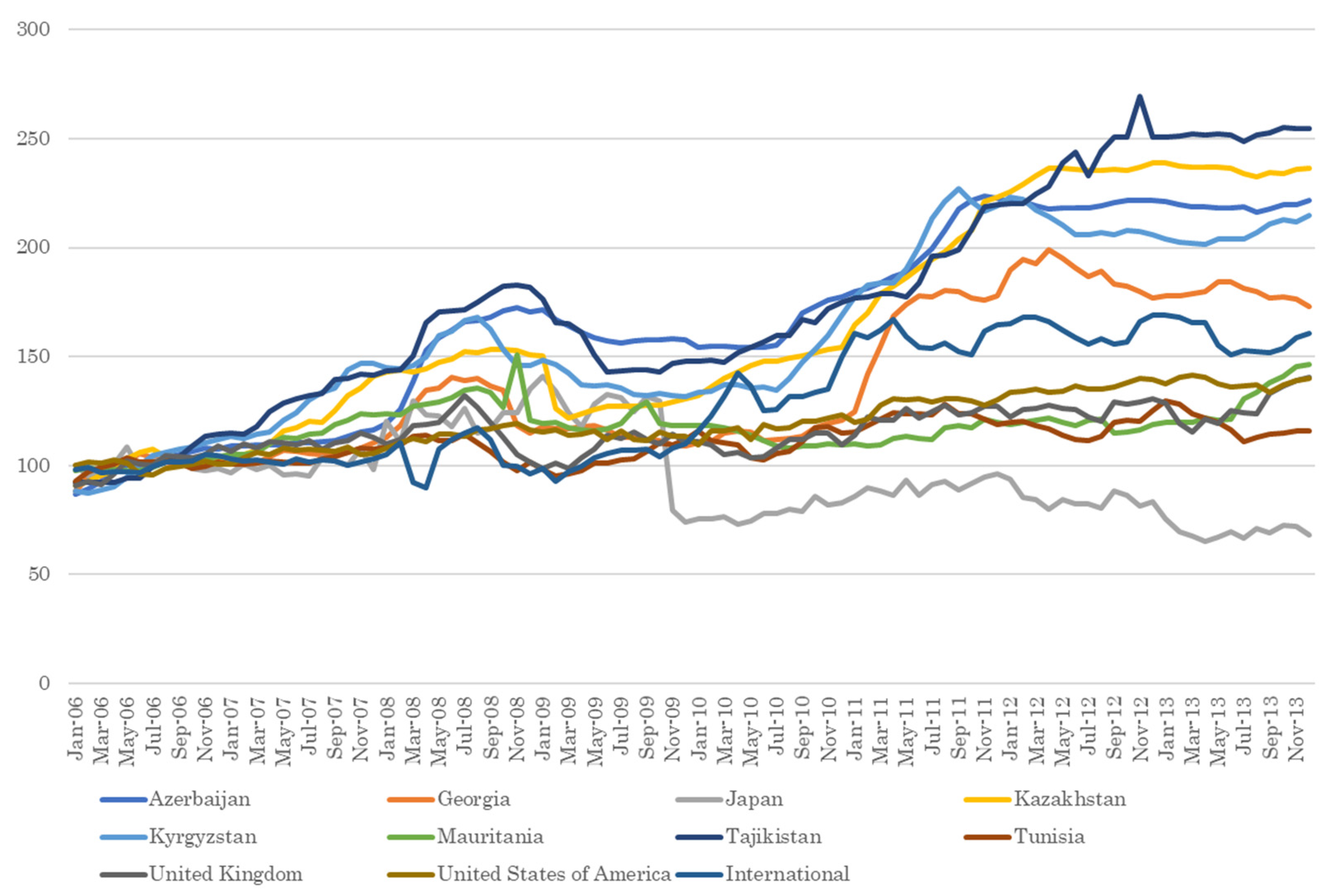
From a historical perspective, infectious animal disease outbreaks, the malfunction of value chains and transport systems due to pandemics such as COVID-19 or the high price of feed grains have jolted both global and local meat markets [1,2,3] (Figure 1) (Figure 1 shows the dataset used in the present article that does not cover the periods of major pandemics such as the BSE and COVID-19, but the food crisis in 2007–2008). Such unexpected events have even changed food consumption patterns of local citizens, impeding the efficient consumption of the food supply [4]. Due to the psychological effects of the BSE incident that occurred in the 1990s, beef demand dramatically fell in Japan. Simultaneously, the BSE scare tightened beef supply to the international markets [5]. In the UK, the retail beef price decreased by 11%, and consumption fell by 24%, which increased the price of the substitute good lamb by 23%, with lamb consumption remaining unchanged during the period of the BSE crisis. In the 2008 global commodity boom, cereal prices were spiked by various factors such as high oil prices, biofuels production from food commodities, poor harvests in Australia and Ukraine and export restrictions. The grain price hikes possibly increased meat prices because grain is an essential element of meat production costs [6]. Thus, countermeasures against the vagaries of global food markets have attracted the attention of food-deficit governments.
The Ministry of Agriculture, Forestry and Fisheries of Japan aims at increasing the country’s food self-sufficiency rate (SSR) for securing food supply against unexpected events (See the MAFF website for further details (https://www.maff.go.jp/e/index.html)). Supply stabilization is closely associated with price stabilization, which directed economists to analyze the relationships between SSR and price co-movement [7,8,9,10]. Thus, a food autarky system has been considered to be an important element for shielding internal markets from uncertain aspects of foreign markets. High food self-sufficiency serves to ensure food availability in an emergent situation such as war. In a peacetime economy, local households are coerced into purchasing unreasonably expensive products under protectionist policies such as high import levies and quotas or shouldering enormous debt due to heavy subsidies from incentivizing domestic farmers to produce more goods. Further, autarky policy does not always function as a shock absorber if domestic production is more volatile than foreign production [9]. Protectionism is often criticized by economists because imposing additional restrictions on imports distorts market signals, inducing inefficient resource allocation. Until the early 2000s, global agricultural markets were relatively calm compared with those after 2007, when nations were encouraged to open international borders to gain the benefits of international trade. This movement to open borders is evidenced by the number of free trade agreements (FTA) that became effective during the 1980s and 1990s (JETRO) (FTAs came into force among countries in the 1980s (56) and the 1990s (over 200). See JETRO (https://www.jetro.go.jp/theme/wto-fta/basic.html) for more detail). However, this global trend guided governments toward protectionist policy after the world food crisis in 2008, and many national governments, including India, Qatar, Senegal, Bolivia, the Philippines, Russia and Egypt, were interested in food autarky policy [11]. The government of Japan has also long attempted to boost its self-sufficiency in food to build a steady food supply system for emergencies (Some articles noted that the Ministry of Agriculture, Forestry and Fisheries of Japan aims at lifting the self-sufficiency rate in Japan for political reasons, not for food security [12]). Thus, self-sufficiency policy has been of national interest among policymakers.
Although the literature on food self-sufficiency policy is substantial [11,13,14,15], only a limited number of papers have attempted to quantify the effects of the policy measure for the cereal sectors. Tanaka [8] and Tanaka and Guo [9] used a global-scale, stochastic general equilibrium framework for the wheat industry to evaluate the usefulness of the self-sufficiency measure in Egypt and Japan, respectively. Guo and Tanaka [7] established a generalized autoregressive conditional heteroskedasticity (GARCH) model with multivariate dynamic conditional correlations (DCC) to estimate the interconnectivity across the global wheat price and regional prices for net importers of wheat flour. With the DCC estimated by the model, the authors used a panel regression model to determine that cross-border price volatility transmissions and self-sufficiency rates are negatively correlated. To our knowledge, no study exists that quantitatively assesses the effectiveness of self-sufficiency for any type of meat.
The literature on price passthroughs of agricultural commodities is bountiful, with approximately 500 articles resulting from an AgEcon search using the phrase “price transmission” [16]. Several papers on beef price transmission concentrate on vertical price transmissions, such as the connections across wholesale and retail prices, as well as a study comparing producer and retail prices in a single country [2,17,18,19,20,21] (AgEcon is “a cooperative project of the University of Minnesota Libraries, the Department of Applied Economics at the University of Minnesota and the Agricultural and Applied Economics Association.” https://ageconsearch.umn.edu/pages/?page=about). Dong et al. [22] and Ghoshray [23] scrutinized international market linkages, but they did not specify the underlying determinants for the intensity of international price volatility transmission, which we identify as a measure of self-sufficiency. In contrast, several studies inspect the volatility of transmissions of price from global to indigenous markets [24,25,26] by applying a vector error correction model (VECM). However, these studies did not explore the extent of time-varying linkages across international and indigenous prices.
This paper analyzes the relationships between international and retail prices of beef for Azerbaijan, Georgia, Japan, Kazakhstan, Kyrgyzstan, Mauritania, Tajikistan, Tunisia, the UK and the United States, as well as the associations between the extent of international price volatility transmissions and autarky rates in beef over the sample period from Jan 2006 to Dec 2013. Our experimental procedure is as follows. First, we gauge the price volatility for each country using univariate exponential GARCH (EGARCH) models and identify lead–lag causal links between world and regional prices by applying a nonuniform weighting cross-correlation function (CCF). Second, dynamic correlations in volatility spillover between global and local beef markets are estimated using a multivariate DCC-EGARCH model. Third, we apply three types of panel models to examine the effects of the self-sufficiency rate (SSR) on international price volatility passthroughs. Further, we also explore the effects of consumption of potential substitutive goods such as pork and chicken and macroeconomic variables such as GDP per capita growth rate on international price volatility transmissions (i.e., DCCs). Guo and Tanaka [7] and Tanaka and Guo [10] conducted a panel analysis for wheat introducing rice and maize consumption variables as substitutes that could mitigate international spillover effects from global wheat market. Bekkers et al. [27] investigated the impacts of GDP per capita on cross-border passthroughs of food prices. Yang et al. [28] identified the macroeconomic factors such as GDP and CPI that can influence DCCs between oil prices and exchange rates by applying a panel regression.
Our article makes contributions to the existing research by providing empirical evidence that self-sufficiency policy could assuage the spillover effects from the international beef market, an observation that had not been elucidated in previous studies. Second, whereas many price transmission papers adopted a VECM, DCC-EGARCH models were employed in this work, which allow for visualization and identification of time-varying price volatility associations between markets. Finally, we succeeded in identifying the causal and lead–lag associations between global and regional beef markets by the CCF method.
The plan of the present paper is as follows: the next section provides a description of the data. Section 3 introduces the econometric methods applied to the analyses and Section 4 presents the experimental outcomes. The outcomes obtained are discussed in Section 5. Finally, we summarize the paper with the limitations of the research and topics to be addressed in future studies.
2. Data and Sample Statistics
In this study, we selected Azerbaijan (AZE), Georgia (GEO), Japan (JPN), Kazakhstan (KAZ), Kyrgyzstan (KGZ), Mauritania (MRT), Tajikistan (TJK), Tunisia (TUN), the United Kingdom (UK) and the United States of America (USA) as net-importing regions of beef based on the criterion that the SSR represents 100% or less, as calculated by the Food and Agriculture Organization (FAO). For the country selection, we also paid attention to the data size in panel analysis (namely, the length of sample period multiplied by the number of net-importing regions). To date, the data availability of monthly local beef price series is highly limited. Accordingly, we did not include major players in the market, such as China. Furthermore, choosing countries with a high or low SSR is desirable in terms of that we conduct panel data analyses. The data for each component of SSR were sourced from the FAOSTAT (http://www.fao.org/faostat/en/#home), and the sample period was from January 2006 to December 2013. Data sources of monthly retail beef price series in US dollar terms for Azerbaijan, Georgia, Kazakhstan, Kyrgyzstan, Mauritania, Tajikistan and Tunisia were retrieved from the FAO’s global information and early warning system (http://www.fao.org/giews/en/). For Japan, we collected the retail price of sirloin beef from Kouribukkatoukei issued by the Statistics Bureau of Japan. For the UK, the retail price of home-killed best beef mince was taken from the UK. Office for National Statistics and for the United States, the retail price of boneless beef for stew was taken from the US Bureau of Labor Statistics. To remove the effect of exchange rates, the data series for Japan and the UK were converted into US dollar units with the exchange rate acquired from the Federal Reserve Economic Data (https://fred.stlouisfed.org/). The international beef prices (IBP) were obtained from International Monetary Fund commodity prices (https://www.imf.org/en/Research/commodity-prices).
All data on prices were adjusted using the X-13-autoregressive integrated moving average (ARIMA) (The X-13-ARIMA program from the US Census Bureau, which is the most popular methodology used around the world) method to eliminate the influence of seasonal fluctuations. Regarding the return series, a first-order logarithmic difference was used for each price series and calculated as , where is the monthly beef price return at time t and is the beef price at time t. The descriptive statistics for all of the monthly returns on beef prices are reported in Table 1. Our findings show that the mean of monthly returns is close to zero for each price. Kazakhstan and Tajikistan demonstrate the highest mean returns, whereas the lowest is for Japan. Note that returns of the IBP are more volatile than all domestic prices, evidenced by the largest standard deviation. Furthermore, Mauritania’s price returns show a relatively higher standard deviation than the other countries. These results are confirmed by the higher range of IBP and Mauritania’s price returns (maximum–minimum). In terms of the asymmetry tests, the skewness suggests evidence of asymmetry, which approaches zero for some price returns (e.g., Georgia, Kyrgyzstan and the UK). The kurtosis test, however, exhibits a leptokurtic excess (i.e., fat-tail distribution) in some price returns (e.g., IBP, Kazakhstan and Mauritania). The Jarque–Bera statistics reject normality at the 1% significance level for most of the price returns, except for Kyrgyzstan, Tunisia and the United States.
Before constructing the econometric model, a stationary process of each price return should be tested using the augmented Dickey–Fuller (ADF) [29], Phillips and Perron (PP) [30] and Kwiatkowski–Phillips–Schmidt–Shin (KPSS) [31] unit root tests. Table 2 reports the results of unit root tests and indicates that all price returns in their first log-differenced form are stationary processes (The ADF, PP and KPSS unit root tests, not reported, indicate that each price of monthly returns in their level are non-stationary). Additionally, the results of a serial autocorrelation test (ARCH–Lagrange multiplier (LM)) indicate the presence of serial correlation and an ARCH effect in all price returns, except for Georgia.
In the panel analysis, we use the annualized SSR of beef in each beef-importing country defined as Production/(Production + Import − Export). Table 3 provides descriptive statistics for SSR. As shown in Table 3, the SSR reveals distinct features in different beef-importing countries. For instance, the average SSR values of Azerbaijan, Kazakhstan, Kyrgyzstan, Tajikistan, Tajikistan, Tunisia and the United States are very high (close to 1), whereas the SSR of Japan shows the lowest values in mean and median. It is also worth noting that the standard deviations of SSR for Georgia and the UK are larger than for the other countries.
3. Econometric Methodology
In the first step, we fit a univariate model to each return of beef prices, which allows for time-varying conditional mean and variance. Since the advent of multivariate GARCH-type modeling [33], the technique has been widely applied to analyze the issue of volatility spillover mechanisms between macroeconomic and financial variables [34,35,36]. In particular, Nelson [37] suggested that the EGARCH model not only ensures the non-negative nature of coefficients in ARCH terms, but also captures the presence of asymmetry in volatility. Accordingly, the autoregressive (AR)-EGARCH model is employed as our econometric model to investigate the time-varying price volatility and the volatility transmission between the IBP and domestic beef price in beef-importing countries. The empirical model can be specified as follows (Equations (1) and (2)):
Equation (1) specifies the conditional mean equation, where is the beef price return and is the information set in time t − 1. The error term is assumed to follow a conditionally normal distribution, with its conditional variance and is an independently and identically distributed (i.i.d.) random error. Equation (2) defines the conditional variance equation, where q and p are the number of GARCH terms and ARCH terms, respectively. We carry out the lag selections using the Bayesian information criterion (BIC) and determine the optimal univariate model for each price return.
In the second step, the CCF approach advocated by Hong (2001) [38] is employed to identify the direction of causality between global and local beef prices in a bivariate framework. Specifically, the standardized residuals (The hats reveal the suitable estimates of the corresponding variables) for international price and for the domestic price can be estimated using the AR-EGARCH model. Then, we can estimate the sample cross-correlation coefficient with the lag order i between the standardized residuals. Hong [38] suggested that the following test statistic can be used to test for causality (Hong [38] performed Monte Carlo experiments and showed that the truncated kernel gives approximately similar power to the Bartlett, Daniell and QS kernels. Following Hong [38], we chose the truncated kernel, which provides compact formation—Equation (3)).
In Equation (3), T is the sample size, is a weighting function, and M is a positive integer. The null hypothesis of no causality in the mean or the variance will be rejected if the test statistic is larger than the critical value of a standard normal distribution (N (0, 1)).
In the third step, we use a bivariate EGARCH model with a conditional variance–covariance matrix to estimate the DCCs between international and domestic beef prices, examining volatility transmissions for each price pair. Following Engle [39], we constructed an econometric framework for a DCC-EGARCH model as follows (Equations (4)–(8)):
is a 2 × 2 conditional variance–covariance matrix of the vector of residuals conditional . is a diagonal matrix containing the conditional standard deviations of each price return. The conditional variance and follow the AR-EGARCH, as described in Equations (1) and (2). represents the time-varying DCC matrix. In Equation (8), is the conditional correlation matrix of the standardized residuals, which can be defined by (Equation (9)):
where “” indicates the Hadamard product parameters. a and b are non-negative parameter matrices with a restriction of to ensure stationarity and positive definiteness of . is the unconditional correlation matrix of the standardized residuals . Cappiello et al. (2006) [40] modified the DCC model and introduced the asymmetric term into the model (The advantages of these models are described by [40]). The authors then constructed an asymmetric, generalized DCC (AG-DCC) model, as in the following expression (Equation (10)):
where A and B are parameter matrices. represents the unconditional matrices of (where is an indicator function equal to 1 if and 0 otherwise) and . The asymmetric DCC (A-DCC) is a special case of the AG-DCC if the matrices are replaced by scalars. The scalar A-DCC model can be expressed by (Equation (11)):
We estimate the vector and by replacing them with a sample analog, and . Moreover, if matrix in Equation (10) equals zero, then the generalized DCC model (G-DCC) can be obtained as follows (Equation (12)):
We use the Gaussian quasi-maximum likelihood estimation (QMLE) to estimate all the parameters of the DCC, A-DCC, AG-DCC and G-DCC models and assume conditional multivariate normality with the Broyden, Fletcher, Goldfarb and Shannon (BFGS) (BFGS is an algorithm from the quasi-Newton second-derivative line search family method, one of the most powerful approaches for solving unconstrained optimization problems. All DCC-EGARCH model estimations were performed using WinRats Professional 10.0) optimization algorithm. Finally, we specified the conditional correlation matrix as . Thus, the conditional correlation at time t can be defined as (Equation (13)):
In the last step, we selected the best model specification based on the BIC and estimated the DCCs between global and local price for each beef-importing country.
To investigate the effects of beef self-sufficiency rates and other determining factors on the DCCs, the following panel regression model was constructed (Equation (14)):
where is the dynamic conditional correlations between international beef price and country i’s domestic beef price at time t. c is the constant term. is the self-sufficiency rate of beef in country i at time t. To consider the other important determinates for DCCs, apart from , we use the variables , and which represent the change rate of domestic consumption (The data for consumption of beef, pork and chicken were sourced from the FAOSTAT) for beef, pork and chicken in country i at time t, respectively. We choose and because the consumption of these meats may have substitutive effects on beef, thereby affecting DCCs of beef. Further, we also apply the variables and which represent the inflation rate and GDP per capita growth rate (The data for consumption of beef, pork and chicken were sourced from the FAOSTAT) in country i at time t. It is reasonable to assume that such important macroeconomic variables in beef-importing countries would influence the dynamics interactions between the global and local beef price. is the heteroskedastic error term. The parameters to measure the effects of each underlying factor that influences the . Moreover, because the SSR data are only available at yearly frequencies, the estimated monthly DCCs for each country are converted into annualized average series (According to David and Amir [41], annualized DCCs can be taken by the average of the monthly DCCs). Furthermore, to solve the problem of data limitation, we treated 10 countries as one and proceeded with the panel analysis.
4. Empirical Results
First, this section investigates causality and lead–lag spillover between international and domestic beef prices. Second, we present the estimates of the degree of DCCs between global and local beef markets. Third, we examine whether the SSR affects beef price transmission in beef-importing countries.
4.1. Causal Relationships and Analysis of Lead–Lag
Initially, the AR (1)-EGARCH (1,1) model was selected for each price return because the model had the lowest BIC value (We follow the method of Hansen and Lunde [42] and Tamakoshi and Hamori [43] to select the optimal lags for the AR-EGARCH model. Table 4 provides details regarding the model selection). The estimation results for each AR-EGARCH model are summarized in Table 4. All estimators of the ARCH () and GARCH () were statistically significant, thereby providing evidence of volatility clustering in each price return. Moreover, it was noticeable that the asymmetric () terms were statistically significant for the price returns of IBP, Azerbaijan, Georgia and Tunisia. These results indicate that the “leverage effect” (negative shocks tend to increase the volatility) is exerted on these four price returns. In addition, Table 4 provides the diagnostics of the estimation of the AR-EGARCH model. The Ljung–Box [44] statistics and ARCH-LM tests suggest that autocorrelation and ARCH effects in all price returns are not present. These results imply that the selected AR-EGARCH model specifications are suitable for the data series. Furthermore, we estimated the standardized residual for each price return and plotted it in Figure 2.
Next, we examined the causality and lead–lag relationship between international and domestic beef prices using the CCF approach. The results are reported in Table 5. We chose the shortest lag length of five (M = 5) to examine the causality-in-mean and causality-in–variance (As mentioned by Hong, one may like to try several different lags or use “rule of thumb” to determine an appropriate lag order (M). Since the nonuniform kernel function naturally discounts higher order lags, as a robustness check, we performed the causality tests by using lags 10 (M = 10) and lags 15 (M = 15). The three different choice of lags produce vary similar results in terms of statistical significance. Therefore, we chose the shortest lag length (M = 5) in our paper). Generally, we can confirm that different causality relationships exist across different countries. First, we cannot verify the statistically significant evidence of causality in mean and variance from IBP to domestic beef prices in Azerbaijan, Kazakhstan, Kyrgyzstan, Mauritania, Tajikistan and Tunisia, and vice versa. This result implies that there are no lead–lag spillovers between IBP and local beef prices in these countries. Second, our findings demonstrate that a unidirectional causality-in-mean exists from IBP to domestic prices in Georgia, the UK and the United States. These results indicate that IBP can serve as a leading indicator of domestic beef prices in these three counties with approximately a five-month lag. Based on these results, the domestic beef prices of Georgia, the UK and the United States lag by five months to reflect the price transmission from the global market to the domestic market. Third, it is interesting to identify a bidirectional causality-in-mean between global and local beef prices in the case of Japan. This finding suggests that Japan’s beef price also affects international beef prices and implies that the former volatility of Japan’s beef market is important in predicting future volatility of the global beef market. We will discuss the above results in further detail below.
4.2. Time-Varying Dynamic Conditional Correlations
Before estimating the time-varying dynamic correlations by maximizing the log-likelihood functions mentioned in the methodology section, the most appropriate DCC model for each price pair should be selected. The BIC reveals that the standard DCC model possessed the best fitting ability for Georgia, Japan, Kazakhstan and Kyrgyzstan (The results of model selection base on BIC were not reported here, but they are available upon request) Meanwhile, the A-DCC model is selected for Tunisia, and the G-DCC model is selected for Azerbaijan, Mauritania, Tajikistan, the UK and the United States. However, the AG-DCC is not suitable for any price pairs. Table 6 presents the results of the estimation of the parameters for all selected models. We can identify that the estimated coefficients on a and b are each significantly positive. These estimated coefficients are non-negative with a sum of less than one in all the models, indicating that the DCCs are mean-reverting. Additionally, the estimated asymmetric term g is negative and statistically significant in A-DCC models for Tunisia, indicating an asymmetric response in correlation.
According to the above model specifications’ selection, we calculated DCCs between international and 10 beef-importing countries’ beef markets. All the pairs of correlations are plotted in Figure 3. Accordingly, the figure shows that DCCs vary over time and display various characteristics across different countries. Specifically, DCCs appear to be higher for Azerbaijan, Japan, Tajikistan and the UK but are more stable for Kazakhstan and the United States. Note that the DCCs of Japan show almost positive values throughout the entire sample period and relatively high values in recent years. From Table 3, we verified that the SSR of beef in Japan is relatively lower than for the other beef-importing countries. Therefore, Japan’s beef demand has considerable effects on the global beef market. Moreover, the increase in DCCs provided sufficient evidence to support our results that Japan’s beef price plays a crucial role in leading the IBP and vice versa. Moreover, our findings indicate that DCCs in some countries (e.g., Azerbaijan, Georgia, Kazakhstan, Tunisia and the United States) fluctuated dramatically during 2007–2008, which may be explained by the turmoil characterizing the global food crisis and financial crisis over the period. For instance, it is interesting that the DCCs of the United States demonstrated a notable fluctuation after the Lehman Brothers’ collapse in 2008, suggesting that the financial crisis had significant impacts on the interrelationship between international and domestic beef prices in the United States.
In addition, we report the descriptive statistics of DCCs for all countries in Table 7. Table demonstrates that the magnitude of the mean and median of DCCs range from approximately −0.006 for the United States to 0.361 for Japan. These findings provide evidence of weak co-movements and interdependency between the domestic market of beef-importing countries and the global beef market. Specifically, Japan has the highest mean and median value of DCCs, providing further evidence of strong co-movements and interdependency between Japan’s domestic market and the global beef market. In contrast, the mean and median of Tunisia and the United States exhibit a lower value of DCCs than for the other counties. Moreover, DCCs in Tajikistan and the UK represent larger fluctuations (highest standard deviation of 0.223), and the United States has the most stable DCC, evidenced by the lowest standard deviation (0.099).
4.3. The Effect of Self-Sufficiency Rates on Dynamic Conditional Correlations
Finally, we investigate how SSRs of beef and other potential factors affect the DCCs in beef-importing countries by applying a panel data analysis. Before estimating the panel regression in Equation (14), we employed some pretests to identify the presence of heteroskedasticity, serial correlation and cross-sectional dependence (CD) in the panel model. Specifically, the Wald [45], Pesaran’s CD [46], and Wooldridge [45] tests were applied to examine heteroskedasticity, cross-sectional correlation and autocorrelation, respectively. The null hypothesis of the Wald test is no heteroskedasticity, whereas that of the CD and Wooldridge tests is cross-sectional independence and no autocorrelation, respectively. The results of these tests are summarized in Table 8, which shows that there is both autocorrelation and heteroskedasticity in the error term, but no cross-sectional dependencies in our panel data model.
For robustness, we applied three different types of methodologies to perform the panel data regression. Naturally, the standard pool ordinary least-squares (OLS) model is taken as the benchmark. The feasible generalized least-squares (FGLS) model is also used by considering heteroskedasticity and autocorrelation (Baltagi [47] suggested that the FGLS model provides stronger estimated power than the pool OLS model.). Furthermore, the Prais–Winsten regression with panel-corrected standard errors (PCSEs) was adopted simultaneously to verify the robustness of our empirical results. Beck and Katz [48] suggested that the PCSE model demonstrates a better estimation performance than the FGLS model.
Table 9 reports the panel data analysis results based on these three different models. It is clear from Table 9 that the coefficients are statistically significant for all models. These findings provide convincing evidence that the SSR of beef plays a crucial role in affecting the DCCs between international and domestic beef prices in 10 beef-importing countries. Moreover, we can also identify that the coefficients of SSR are significantly negative in each model specification. These findings reveal that an increase in SSR will substantially alleviate shocks and volatility transmissions between the global and domestic beef markets. Therefore, beef-importing countries may refine their strategies for increasing their SSR, which could be a useful instrument for hedging the risk of excessive volatility in international beef prices. This finding is consistent with Guo and Tanaka [7], who found that a higher SSR for wheat in importing countries plays a vital role in extenuating volatility transmissions from global to local wheat prices. On the other hand, it was verified that the coefficients of PORK () and CHIKEN () are not significant even at the 10% level in all three models. These findings indicate that the consumption of pork and chicken did not have significant impacts on the dynamic correlations between global and local beef price. Such results may be due to the different food cultures and religions of particular countries (e.g., Tunisia and Mauritania are Islamic countries; hence, pork is consumed rarely). Finally, we can observe that the coefficients of CPI () and GDP () are also statistically insignificant in all cases, implying that macroeconomic factors did not have explanatory power for volatility transmission of beef prices in beef-importing countries. These findings are different from those of Guo and Tanaka [7], who observed that CPI had a significant negative and GDP had a significant positive effect on DCCs between international and domestic wheat prices.
5. Discussions
Regarding the outcomes of our experiments, we first found that Georgia, the UK and the United States have a unilateral causality from international to individual regional markets. Local markets in the other countries studied were not affected by the global market, except Japan, where the local price influences the international price. These results present an interesting contrast to the findings of Guo and Tanaka [7], in which interconnections were probed between global wheat prices and wheat flour retail prices in net importers. In [7], a unilateral causal linkage from international to local prices was confirmed for all 10 regions selected, with a five-month lag. The cross-border links in the beef sector analyzed in the present paper appear to be weaker than those in the wheat sector, a result that is partly due to the heterogeneity of industrial systems between the two sectors. In particular, animal meat production is adjustable by deciding upon the number of livestock animals to be slaughtered, whereas the grain harvest heavily depends on weather conditions; therefore, production levels cannot be easily altered. Accordingly, international price volatility transmissions in the beef sector seem to be smaller than those in the wheat sector, buffering shocks in global or foreign markets through the flexible adjustment of local production.
Second, Japan was found to be the only region where a bidirectional relationship exists from local to international prices. Japan is the third-largest importing nation with a 9% import share of the global beef market in 2017 (FAOSTAT). Japan’s averaged self-sufficiency rate during the period concerned was 45%, which is by far the lowest among the 10 regions we selected for this analysis. In 2019, Japan and the United States concluded an international trade agreement that lowers Japanese import tariff rates on agricultural products such as beef, pork and cheese exported from the United States [49]. The current 38.5% import levy imposed on beef will be reduced to only 9% by 2033. Accordingly, Japan is likely to have more influential power on international beef prices in the future.
Finally, it was also found that high self-sufficiency in beef has the effect of isolating domestic markets from international markets. Production subsidies to domestic farming operators or raising import tariffs on beef products would be effective in elevating autarky rates. These types of policies improve food availability and access under emergent situations such as the COVID-19 pandemic, extremely poor harvests in exporting countries or wars. However, actualizing autarky is generally a costly policy that sacrifices opportunities to purchase cheaper goods in peacetime, thereby deteriorating the efficiency of resource allocation. Whether a self-sufficiency measure is implemented relies on consumers’ preferences for risk and the frequency of the occurrence of crises in external markets.
6. Conclusions
This paper examined international price volatility transmissions in the beef markets to identify the effectiveness of self-sufficiency as a determinant of international price volatility passthroughs. Our primary findings are as follows. First, unidirectional causality running from global to local markets was observed for Georgia, the UK and the United States, and bidirectional causality was found for Japan. Second, we determined that interconnectivity between global and local beef prices tends to be relatively lower compared with that of wheat, and the degree of market associations shows a tendency to be higher around the 2007–2008 global food and financial crisis. Finally, it was found that higher self-sufficiency could insulate domestic from global markets.
According to statistics from the FAOSTAT, global beef consumption has been increasing, while per capita consumption in the world has been declining since around the 1970s. Per person consumption in developing nations, Japan and South Korea is tending to rise. In contrast, such consumption falls in many Western countries, which may have been caused by environmental factors such as methane emission by cattle and increased vegetable consumption as a substitute by preference over health-conscious lifestyles. Assuming that a certain importing country maintains its SSR, such a reduction of domestic consumption leads to lower domestic production. If domestic consumption is limited, the welfare losses or market distortion entailed by protectionist policy would also be small.
In our analyses, just 10 importing countries were selected, taking into account the data size in panel data analysis due to the fact that local price data series are limitedly available. Needless to say, more countries and a longer sample period enable us to make higher credible estimates. Although our outcomes maintain the robustness by testing with various methods, future studies could attempt to analyze international market connections to validate the conclusions.
Although this paper found that high self-sufficiency is effective in assuaging the spillover effects from the global beef market, we did not analyze the cost-effectiveness of beef autarky policy, which is an essential process before enforcing policies. Generally, a large national budget would be required to improve self-sufficiency through import tariffs or farming subsidies to local farmers. Simulation models, such as computable general equilibrium models, make it possible to estimate policy implementation costs. For example, the policy benefit can be gauged with the Arrow–Pratt coefficient, which enables probabilistic effects to be converted into monetary value [50]. These subjects are left for future research.
Author Contributions
Conceptualization, T.T. and J.G.; methodology, J.G.; software, J.G.; validation, J.G. and T.T.; formal analysis, J.G. and T.T.; investigation, J.G. and T.T.; resources, J.G. and T.T.; data curation, T.T.; writing—original draft preparation, J.G. and T.T.; writing—review and editing, J.G. and T.T.; visualization, J.G.; supervision, J.G. and T.T.; project administration, T.T.; funding acquisition, T.T. All authors have read and agreed to the published version of the manuscript.
Funding
The research is, in part, supported by a Grant-in-Aid from the Japan Society for the Promotion of Science (Grant Number (A) 20K15613).
Conflicts of Interest
The authors declare no conflicts of interest.
References
- Conner, K. Is There Really a Meat Shortage? Why You’re Seeing Less Beef, Pork, and Chicken in Stores. CNET. 3 June 2020. Available online: https://www.cnet.com/health/is-there-really-a-meat-shortage-why-youre-seeing-less-beef-pork-and-chicken-in-stores/ (accessed on 10 June 2020).
- Sanjuán, A.I.; Dawson, P.J. Price transmission, BSE and structural breaks in the UK meat sector. Eur. Rev. Agric. Econ. 2003, 30, 155–172. [Google Scholar] [CrossRef]
- Lawrence, J.D.; Mintert, J.; Anderson, J.D.; Anderson, D.P. Feed grains and livestock: Impacts on meat supplies and prices. Choices 2008, 23, 11–15. [Google Scholar]
- Peterson, H.H.; Chen, Y.J. The impact of BSE on Japanese retail beef market. Agribusiness 2003, 21, 313–327. [Google Scholar] [CrossRef]
- Ishida, T.; Ishikawa, N.; Fukushige, M. Impact of BSE and bird flu on consumers’ meat demand in Japan. Appl. Econ. 2010, 42, 49–56. [Google Scholar] [CrossRef]
- Tanaka, T.; Hosoe, H.; Qiu, H. Risk Assessment of Food Supply: A Computable General Equilibrium Approach; Cambridge Scholars Publishing: Newcastle upon Tyne, UK, 2012. [Google Scholar]
- Guo, J.; Tanaka, T. Determinants of international price volatility transmissions: The role of self-sufficiency rates in wheat-importing countries. Palgrave Commun. 2019, 5, 1–13. [Google Scholar] [CrossRef]
- Tanaka, T. Agricultural self-sufficiency and market stability: A revenue-neutral approach to wheat sector in Egypt. J. Food Secur. 2018, 6, 31–41. [Google Scholar] [CrossRef] [Green Version]
- Tanaka, T.; Guo, J. Quantifying the effects of agricultural autarky policy: Resilience to yield volatility and export restrictions. J. Food Secur. 2019, 7, 47–57. [Google Scholar] [CrossRef]
- Tanaka, T.; Guo, J. How does the self-sufficiency rate affect international price volatility transmissions in the wheat sector? Evidence from wheat-exporting countries. Humanit. Soc. Sci. Commun. 2020, 7, 1–13. [Google Scholar] [CrossRef]
- Clapp, J. Food self-sufficiency: Making sense of it, and when it makes sense. Food Policy 2017, 66, 83–96. [Google Scholar] [CrossRef] [Green Version]
- Tanaka, T.; Hosoe, N. Does agricultural trade liberalization increase risks of supply-side uncertainty? Effects of productivity shocks and export restrictions on welfare and food supply in Japan. Food Policy 2011, 36, 368–377. [Google Scholar] [CrossRef]
- Bishwajit, G. Food security and food self-sufficiency in China: From past to 2050. Food Energy Secur. 2014, 3, 86–95. [Google Scholar]
- Clarete, R.L.; Adriano, L.; Esteban, A. Rice Trade and Price Volatility: Implications on ASEAN and Global Food Security. ADB Economic Working Paper Series No. 368. 2013. Available online: https://www.adb.org/sites/default/files/publication/30390/ewp-368.pdf (accessed on 20 June 2020).
- Warr, P. Food Security vs. Food Self-Sufficiency: The Indonesian Case. Crawford School Research Paper No. 2011/04. 2011. Available online: https://papers.ssrn.com/sol3/papers.cfm?.abstract_id=1910356 (accessed on 10 January 2018).
- Kouyaté, C.; von Cramon-Taubadel, S. Distance and border effects on price transmission: A meta-analysis. J. Agric. Econ. 2016, 67, 255–271. [Google Scholar] [CrossRef] [Green Version]
- Bakucs, L.Z.; Fertö, I. Marketing margins and price transmission on the Hungarian beef market. Food Econ. 2006, 3, 151–160. [Google Scholar]
- Fousekis, P.; Katrakilidis, C.; Trachanas, E. Vertical price transmission in the US beef sector: Evidence from the nonlinear ARDL model. Econ. Model. 2016, 52, 499–506. [Google Scholar] [CrossRef]
- Goodwin, B.K.; Holt, M.T. Price transmission and asymmetric adjustment in the U.S. beef sector. Am. J. Agric. Econ. 1999, 81, 630–637. [Google Scholar] [CrossRef]
- Pozo, V.F.; Schoroeder, T.C.; Bachmeier, L.J. Symmetric Price Transmission in the U.S. Beef Market: New Evidence from New Data. In Proceedings of the NCCC-134 Conference on Applied Commodity Price Analysis, Forecasting, and Market Risk Management, St. Louis, MO, USA, 22–23 April 2013; Available online: http://www.farmdoc.illinois.edu/nccc134 (accessed on 15 April 2020).
- Saghaian, S.H. Beef safety shocks and dynamics of vertical price adjustment: The case of BSE discovery in the U.S. beef sector. Agribusiness 2007, 23, 333–348. [Google Scholar] [CrossRef]
- Dong, X.; Waldron, S.; Brown, C.; Zhang, J. Price transmission in regional beef markets: Australia, China and Southeast Asia. Emir. J. Food Agric. 2018, 30, 99–106. [Google Scholar] [CrossRef] [Green Version]
- Ghoshray, A. Underlying Trends and International Price Transmission of Agricultural Commodities. In ADB Economics Working Paper Series, No. 257; Asian Development Bank: Metro Manila, Philippines, 2011. [Google Scholar]
- Ceballos, F.; Hernandez, M.A.; Minot, N.; Robles, M. Grain price and volatility transmission from international to domestic markets in developing countries. World Dev. 2017, 94, 305–320. [Google Scholar] [CrossRef]
- Guo, J.; Tanaka, T. Dynamic transmissions and volatility spillovers between global price and U.S. producer price in agricultural markets. J. Risk Financ. Manag. 2020, 3, 83. [Google Scholar] [CrossRef]
- Hatzenbuehler, P.L.; Abbott, P.C.; Abdoulaye, T. Price transmission in Nigerian food security crop markets. J. Agric. Econ. 2017, 68, 143–163. [Google Scholar] [CrossRef]
- Bekkers, E.; Brockmeier, M.; Francois, J.; Yang, F. Local food prices and international price transmission. World Dev. 2017, 96, 216–230. [Google Scholar] [CrossRef]
- Yang, L.; Cai, X.J.; Hamori, S. What determines the long-term correlation between oil prices and exchange rates? N. Am. J. Econ. Financ. 2018, 44, 140–152. [Google Scholar] [CrossRef]
- Dickey, D.A.; Fuller, W.A. Distribution of the estimators for autoregressive time series with a unit root. J. Am. Stat. Assoc. 1979, 74, 427–431. [Google Scholar]
- Phillips, P.C.; Perron, P. Testing for a unit root in time series regression. Biometrika 1988, 75, 335–346. [Google Scholar] [CrossRef]
- Kwiatkowski, D.; Phillips, P.C.B.; Schmidt, P.; Shin, Y. Testing the null hypothesis of stationarity against the alternative of a unit root. J. Econom. 1992, 54, 159–178. [Google Scholar] [CrossRef]
- Newey, W.K.; West, K.D. Automatic lag selection in covariance matrix estimation. Rev. Econ. Stud. 1994, 61, 631–653. [Google Scholar] [CrossRef]
- Bauwens, L.; Laurent, S.; Rombouts, J.V. Multivariate GARCH Models: A Survey. J. Appl. Econ. 2006, 21, 79–109. [Google Scholar] [CrossRef] [Green Version]
- Guo, J. Causal relationship between stock returns and real economic growth in the pre- and post-crisis period: Evidence from China. Appl. Econ. 2014, 47, 12–31. [Google Scholar] [CrossRef]
- Basher, S.A.; Sadorsky, P. Hedging emerging market stock prices with oil, gold, VIX and bonds: A comparison between DCC ADCC and GO-GARCH. Energy Econ. 2016, 54, 235–247. [Google Scholar] [CrossRef] [Green Version]
- Guo, J. Co-movement of international copper prices, China’s economic activity and stock returns: Structural breaks and volatility dynamics. Glob. Financ. J. 2018, 36, 62–77. [Google Scholar] [CrossRef]
- Nelson, D. Conditional heteroskedasticity in asset returns: A new approach. Econometrica 1991, 59, 347–370. [Google Scholar] [CrossRef]
- Hong, Y. A test for volatility spillover with applications to exchange rates. J. Econom. 2001, 103, 183–224. [Google Scholar] [CrossRef]
- Engle, R.F. Dynamic conditional correlation: A simple class of multivariate generalized autoregressive conditional heteroscedasticity models. J. Bus. Econ. Stat. 2002, 20, 339–350. [Google Scholar] [CrossRef]
- Cappiello, L.; Engle, R.F.; Sheppard, K. Asymmetric correlations in the global equity and bond returns. J. Financ. Econ. 2006, 4, 537–572. [Google Scholar] [CrossRef]
- David, L.B.; Amir, R. Stocks and bonds during the gold standard. Econ. Lett. 2017, 159, 119–122. [Google Scholar]
- Hansen, P.R.; Lunde, A. A forecast comparison of volatility models: Does anything beat a GARCH (1,1)? J. Appl. Econ. 2005, 20, 873–889. [Google Scholar] [CrossRef] [Green Version]
- Tamakoshi, G.; Hamori, S. Causality-in-variance and causality-in-mean between the Greek sovereign bond yields and Southern European banking sector equity returns. J. Econ. Financ. 2014, 38, 627–642. [Google Scholar] [CrossRef]
- Ljung, G.M.; Box, G.E.P. On a measure of lack of fit in time series models. Biometrika 1978, 65, 297–303. [Google Scholar] [CrossRef]
- Wooldridge, J.M. Econometric Analysis of Cross-Section and Panel Data; MIT Press: Cambridge, MA, USA, 2010. [Google Scholar]
- Pesaran, M.H. General Diagnostic Tests for Cross-Section Dependence in Panels. In Cambridge Economics Working Paper No. 0435; Cambridge University: Cambridge, UK, 2004. [Google Scholar]
- Baltagi, B.H. Simultaneous equations with error components. J. Econom. 1981, 17, 189–200. [Google Scholar] [CrossRef]
- Beck, N.; Katz, J.N. What to do (and not to do) with time series cross-section data. Am. Political Sci. Rev. 1995, 89, 634–647. [Google Scholar] [CrossRef]
- Kaneko, K.; Sieg, L.; Polansek, T. For U.S. Beef Exporters, Japan Trade Deal Levels Playing Field But Sales Surge Unlikely. Reuters. 26 September 2019. Available online: https://www.reuters.com/article/us-usa-trade-japan-beef/for-u-s-beef-exporters-japan-trade-deal-levels-playing-field-but-sales-surge-unlikely-idUSKBN1WB0ZG (accessed on 8 June 2020).
- Fox, G.; Turner, J.; Gillepie, T. The value of precipitation forecast information in winter wheat production. Agric. For. Meteorol. 1999, 95, 99–111. [Google Scholar] [CrossRef]
Figure 1.
Global and retail price evolution of beef (average of 2006 = 100).

Figure 2.
Plots of standardized residuals for beef price returns.

Figure 3.
Plots of dynamic correlation between global and local beef prices.


Table 1.
Summary statistics for beef price returns.
| Mean | Std. Dev. | Max | Min | Skewness | Kurtosis | Jarque–Bera | |
|---|---|---|---|---|---|---|---|
| IBP | 0.005 | 0.037 | 0.166 | −0.194 | −0.639 | 14.489 | 528.916 *** |
| AZE | 0.009 | 0.018 | 0.091 | −0.025 | 1.763 | 8.688 | 177.291 *** |
| GEO | 0.007 | 0.026 | 0.109 | −0.109 | −0.122 | 7.676 | 86.800 *** |
| JPN | 0.000 | 0.027 | 0.076 | −0.066 | 0.519 | 3.602 | 5.706 * |
| KAZ | 0.010 | 0.025 | 0.070 | −0.169 | −3.561 | 28.609 | 2796.815 *** |
| KGZ | 0.009 | 0.022 | 0.066 | −0.053 | −0.114 | 3.162 | 0.308 |
| MRT | 0.004 | 0.034 | 0.170 | −0.211 | −1.657 | 24.438 | 1862.623 *** |
| TJK | 0.010 | 0.024 | 0.073 | −0.065 | −0.638 | 4.465 | 14.934 *** |
| TUN | 0.002 | 0.022 | 0.053 | −0.053 | −0.235 | 2.987 | 0.878 |
| UK | 0.004 | 0.032 | 0.086 | −0.092 | −0.042 | 3.751 | 2.261 |
| USA | 0.003 | 0.019 | 0.068 | −0.050 | 0.239 | 4.249 | 7.083 ** |
Notes: *, ** and *** denote statistical significance at the 10%, 5% and 1% levels, respectively.
Table 2.
Unit root test and serial autocorrelation test (ARCH–Lagrange multiplier (LM) test.
| ADF | PP | KPSS | ARCH-LM Test | |
|---|---|---|---|---|
| IBP | −8.845 *** (0) | −8.809 *** (3) | 0.107 (4) | 2.502 ** |
| AZE | −3.255 *** (1) | −3.210 *** (1) | 0.052 (6) | 2.230 ** |
| GEO | −6.174 *** (0) | −6.230 *** (3) | 0.083 (2) | 0.101 |
| JPN | −9.134 *** (0) | −9.159 *** (2) | 0.113 (2) | 1.966 * |
| KAZ | −5.880 *** (0) | −5.880 *** (3) | 0.092 (5) | 3.029 * |
| KGZ | −3.993 *** (0) | −3.817 *** (5) | 0.101 (5) | 2.400 * |
| MRT | −13.271 *** (0) | −12.900 *** (4) | 0.171 (2) | 9.879 *** |
| TJK | −2.875 *** (2) | −7.042 *** (5) | 0.101 (5) | 1.772 * |
| TUN | −7.687 *** (0) | −7.701 *** (3) | 0.044 (4) | 3.422 * |
| UK | −9.749 *** (0) | −9.750 *** (3) | 0.055 (2) | 2.892 * |
| USA | −12.733 *** (0) | −12.884 *** (2) | 0.051 (3) | 1.787 * |
Notes: *, ** and *** denote statistical significance at the 10%, 5% and 1% levels, respectively. Numbers in brackets are the lag length and bandwidth. Lag length selection is based on BIC in the ADF tests. The bandwidth for the KPSS test is determined using the Bartlett kernel and Newey–West bandwidth selection algorithm [32]. Based on the BIC, all the unit root tests are implemented with intercept and trend terms. Ten lags are used in the ARCH-LM test.
Table 3.
Summary statistics for the self-sufficiency rates (SSRs) in the panel analysis.
| Mean | Median | Std. Dev. | |
|---|---|---|---|
| AZE | 0.948 | 0.956 | 0.024 |
| GEO | 0.721 | 0.718 | 0.056 |
| JPN | 0.446 | 0.447 | 0.014 |
| KAZ | 0.947 | 0.950 | 0.019 |
| KGZ | 0.972 | 0.971 | 0.013 |
| MRT | 1.000 | 1.000 | 0.000 |
| TJK | 0.970 | 0.967 | 0.013 |
| TUN | 0.924 | 0.918 | 0.013 |
| UK | 0.711 | 0.713 | 0.055 |
| USA | 0.982 | 0.986 | 0.036 |
Notes: The sample data cover the period from 2006 through 2013. The annualized SSR is calculated as Production/(Production + Import − Export).
Table 4.
Empirical results of AR-EGARCH model.
| Parameters | Specification Tests | ||||||||
|---|---|---|---|---|---|---|---|---|---|
| ARCH-LM Test | BIC | ||||||||
| IBP | 0.003 * | 0.128 | −1.623 *** | 0.124 *** | −0.207 * | 0.863 *** | 4.456 | 0.313 | −4.199 |
| AZE | 0.002 ** | 0.714 *** | −5.659 ** | 0.232 ** | 0.487 *** | 0.401 ** | 4.492 | 0.347 | −6.031 |
| GEO | 0.002 | 0.518 *** | −4.828 *** | 0.327 *** | −0.520 ** | 0.632 *** | 3.044 | 0.248 | −4.456 |
| JPN | 0.000 | 0.047 | −13.239 *** | 0.067 ** | 0.223 | 0.848 *** | 3.291 | 0.617 | −4.218 |
| KAZ | 0.008 *** | 0.218 *** | −13.758 *** | 0.101 *** | 0.236 | 0.803 *** | 3.114 | 0.226 | −4.826 |
| KGZ | 0.003 * | 0.712 *** | −13.828 *** | 0.393 * | −0.124 | 0.638 *** | 7.249 | 0.580 | −5.109 |
| MRT | 0.007 *** | 0.025 | −5.403 *** | 0.004 *** | 0.094 | 0.902 ** | 7.115 | 0.512 | −4.607 |
| TJK | 0.009 *** | 0.223 * | −5.166 ** | 0.299 *** | 0.045 | 0.692 ** | 6.282 | 0.712 | −4.517 |
| TUN | 0.004 * | 0.261 *** | −1.173 | 0.169 ** | −0.222 ** | 0.897 *** | 6.604 | 1.068 | −4.800 |
| UK | 0.004 | −0.099 | −6.982 ** | 0.130 ** | −0.159 | 0.867 ** | 12.411 | 0.906 | −3.829 |
| USA | 0.003 ** | −0.113 | −11.950 *** | 0.103 *** | 0.125 | 0.883 *** | 8.039 | 0.533 | −5.025 |
Notes: *, ** and *** denote statistical significance at the 10%, 5% and 1% levels, respectively. We employed the residual diagnostics tests to determine the optimal lag length of AR (k)-EGARCH (p, q) model. Based on the BIC, the lag length in each mean and variance equation are selected from among k = 1, 2 … 10, p = 1, 2 and q = 1, 2, respectively. Diagnostic test: are the Ljung–Box [44] statistics for the null hypothesis of no autocorrelation up to the order of 10 for squared standardized residuals.
Table 5.
Results for Hong’s [38] Granger causality test.
Table 5.
Results for Hong’s [38] Granger causality test.
| Causality from Global Price to Local Price | Causality-in-Mean (M = 5) | Causality-in-Variance (M = 5) | Causality from Local Price to Global Price | Causality-in-Mean (M = 5) | Causality-in-Variance (M = 5) |
|---|---|---|---|---|---|
| IBP → AZE | 0.491 | −1.333 | AZE → IBP | −0.143 | −0.995 |
| IBP → GEO | 1.986 ** | −0.173 | GEO → IBP | 0.300 | −0.122 |
| IBP → JPN | 1.839 ** | 3.051 *** | JPN → IBP | 2.556 *** | −0.560 |
| IBP → KAZ | 0.461 | −1.479 | KAZ → IBP | −1.335 | −0.871 |
| IBP → KGZ | 0.458 | −0.137 | KGZ → IBP | 0.794 | 0.761 |
| IBP → MRT | −0.789 | −0.540 | MRT → IBP | −1.073 | 0.618 |
| IBP → TJK | 0.856 | 0.469 | TJK → IBP | −0.024 | −0.460 |
| IBP → TUN | 0.111 | 0.611 | TUN → IBP | 0.282 | −0.553 |
| IBP → UK | 2.323 *** | 3.052 *** | UK → IBP | 0.487 | −1.255 |
| IBP → USA | 1.938 ** | −0.338 | USA → IBP | −0.216 | 0.367 |
Notes: ** and *** denote statistical significance at the 10% and 5% levels, respectively. The arrow indicates the direction of Granger causality. The Hong [38] statistic is applied to test the null hypothesis of no causality from lag 1 up to lag 5.
Table 6.
Empirical results of four specifications for dynamic conditional correlations (DCC) models.
Table 6.
Empirical results of four specifications for dynamic conditional correlations (DCC) models.
| DCC | A-DCC | G-DCC | BIC | |||||||
|---|---|---|---|---|---|---|---|---|---|---|
| AZE | 0.113 ** | −0.737 *** | 0.876 *** | 0.701 *** | −873.252 | |||||
| GEO | 0.441 *** | 0.519 ** | −739.933 | |||||||
| JPN | 0.551 *** | −0.237 | 0.834 *** | 0.286 | −739.375 | |||||
| KAZ | 0.013 *** | 0.928 *** | −803.753 | |||||||
| KGZ | 0.264 ** | 0.647 ** | −824.018 | |||||||
| MRT | 0.886 *** | −0.062 *** | 0.474 *** | 1.024 *** | −748.935 | |||||
| TJK | 0.405 *** | 0.342 *** | 0.881 *** | −1.009 *** | −812.306 | |||||
| TUN | 0.000 | 0.864 *** | −0.444 ** | −834.120 | ||||||
| UK | 0.270 *** | 0.987 *** | 1.021 *** | −0.127 | −709.671 | |||||
| USA | −0.062 *** | 0.302 *** | −1.019 *** | −0.987 *** | −794.574 | |||||
Notes: *, ** and *** denote statistical significance at the 10%, 5% and 1% levels, respectively.
Table 7.
Summary statistics for dynamic conditional correlations of beef.
| Mean | Median | Maximum | Minimum | Std. Dev. | |
|---|---|---|---|---|---|
| AZE | 0.219 | 0.187 | 0.844 | −0.332 | 0.192 |
| GEO | 0.053 | 0.055 | 0.589 | −0.349 | 0.196 |
| JPN | 0.361 | 0.352 | 0.935 | −0.097 | 0.183 |
| KAZ | 0.187 | 0.212 | 0.591 | −0.359 | 0.222 |
| KGZ | 0.163 | 0.157 | 0.535 | −0.160 | 0.124 |
| MRT | 0.109 | 0.081 | 0.669 | −0.212 | 0.131 |
| TJK | 0.142 | 0.127 | 0.999 | −0.292 | 0.237 |
| TUN | −0.008 | −0.045 | 0.393 | −0.162 | 0.129 |
| UK | 0.152 | 0.112 | 0.998 | −0.420 | 0.233 |
| USA | −0.006 | −0.006 | 0.817 | −0.153 | 0.099 |
Table 8.
Specification tests of panel estimation.
| Modified Wald Test for Group-Wise Heteroskedasticity | Pesaran’s Test of Cross-Sectional Independence | Wooldridge Test for Autocorrelation | |
|---|---|---|---|
| Statistics | 163.880 *** | 0.047 | 3.822 * |
Note: * and *** denote statistical significance at the 10% and 1% levels, respectively.
Table 9.
Estimation results of panel data analysis.
| Pool OLS Model | FGLS Model with Heteroskedasticity and Autocorrelation | Prais–Winsten Regression with PCSEs | |
|---|---|---|---|
| SSR () | −0.385 *** | −0.316 ** | −0.291 *** |
| BEEF () | 0.242 | −0.017 | −0.075 |
| PORK () | −0.144 | −0.071 | −0.096 |
| CHIKEN () | 0.018 | 0.028 | 0.024 |
| CPI () | 0.348 | 0.524 | 0.145 |
| GDP () | −0.045 | −0.052 | −0.074 |
| Constant () | 0.448 *** | 0.378 *** | 0.379 *** |
| 0.171 | – | 0.077 | |
| Wald test | 24.390 *** | 15.31 * | 10.38 ** |
| Observations | 80 | 80 | 80 |
Notes: *, ** and *** denote statistical significance at the 10%, 5% and 1% levels, respectively.
© 2020 by the authors. Licensee MDPI, Basel, Switzerland. This article is an open access article distributed under the terms and conditions of the Creative Commons Attribution (CC BY) license (http://creativecommons.org/licenses/by/4.0/).
Share and Cite
MDPI and ACS Style
Guo, J.; Tanaka, T. The Effectiveness of Self-Sufficiency Policy: International Price Transmissions in Beef Markets. Sustainability 2020, 12, 6073. https://doi.org/10.3390/su12156073
AMA Style
Guo J, Tanaka T. The Effectiveness of Self-Sufficiency Policy: International Price Transmissions in Beef Markets. Sustainability. 2020; 12(15):6073. https://doi.org/10.3390/su12156073
Chicago/Turabian StyleGuo, Jin, and Tetsuji Tanaka. 2020. "The Effectiveness of Self-Sufficiency Policy: International Price Transmissions in Beef Markets" Sustainability 12, no. 15: 6073. https://doi.org/10.3390/su12156073
Note that from the first issue of 2016, this journal uses article numbers instead of page numbers. See further details here.