
In Situ Observation-Constrained Global Surface Soil Moisture Using Random Forest Model
by
 , , , ,
Lijie Zhang
1,†, 
Yijian Zeng
1,
Ruodan Zhuang
1,2,
Brigitta Szabó
3,
Salvatore Manfreda
4 ,
,
Qianqian Han
1 and
Zhongbo Su
1,5,* 1
Faculty of Geo-Information and Earth Observation (ITC), University of Twente, 7514 AE Enschede, The Netherlands
2
Department of European and Mediterranean Cultures, Architecture, Environment, Cultural Heritage, University of Basilicata, 75100 Matera, Italy
3
Institute for Soil Sciences, Centre for Agricultural Research, 1022 Budapest, Hungary
4
Department of Civil, Architectural and Environmental Engineering, University of Naples Federico II, 80125 Naples, Italy
5
Key Laboratory of Subsurface Hydrology and Ecological Effect in Arid Region of Ministry of Education, School of Water and Environment, Chang’an University, Xi’an 710054, China
*
Author to whom correspondence should be addressed.
†
Current address: Research Centre Jülich, Institute of Bio and Geosciences: Agrosphere (IBG-3), 52425 Jülich, Germany.
Remote Sens. 2021, 13(23), 4893; https://doi.org/10.3390/rs13234893
Submission received: 1 November 2021
/
Revised: 28 November 2021
/
Accepted: 29 November 2021
/
Published: 2 December 2021
(This article belongs to the Special Issue Global Gridded Soil Information Based on Machine Learning)
Abstract
:The inherent biases of different long-term gridded surface soil moisture (SSM) products, unconstrained by the in situ observations, implies different spatio-temporal patterns. In this study, the Random Forest (RF) model was trained to predict SSM from relevant land surface feature variables (i.e., land surface temperature, vegetation indices, soil texture, and geographical information) and precipitation, based on the in situ soil moisture data of the International Soil Moisture Network (ISMN.). The results of the RF model show an RMSE of 0.05 m3 m−3 and a correlation coefficient of 0.9. The calculated impurity-based feature importance indicates that the Antecedent Precipitation Index affects most of the predicted soil moisture. The geographical coordinates also significantly influence the prediction (i.e., RMSE was reduced to 0.03 m3 m−3 after considering geographical coordinates), followed by land surface temperature, vegetation indices, and soil texture. The spatio-temporal pattern of RF predicted SSM was compared with the European Space Agency Climate Change Initiative (ESA-CCI) soil moisture product, using both time-longitude and latitude diagrams. The results indicate that the RF SSM captures the spatial distribution and the daily, seasonal, and annual variabilities globally.
1. Introduction
Soil moisture (SM) is an essential climate variable that plays a fundamental role in the water and heat exchanges between the land and atmosphere [1,2,3]. Soil moisture controls the allocating of the precipitation into runoff and infiltration and feedback to the atmosphere [4] via its role in partitioning the incoming radiation into latent, sensible, and ground heat fluxes. In most hydrological models, the initial SSM will significantly impact the climatic mean and predicted extremes [5]. Thus, predicting and analyzing the surface soil moisture (SSM) at a global scale will contribute to understanding the hydrological cycle, land surface processes, and land-atmosphere interactions.
So far, there are three main methods for obtaining SSM: in situ measurements, remote sensing (RS)-based retrievals, and land surface model (LSM) simulations, each of which has its advantages and limitations. The in situ measurements could provide continuous SM time series from different soil layers at the point scale. There are community efforts in developing an in situ SM database with global coverage, for example, the International Soil Moisture Network (ISMN) [6,7,8]. Remote sensing has an edge in extensive spatial coverage and is low cost compared to in situ sensors. There are RS-based SSM products from both active (e.g., ASCAT, Sentinel-1) and passive microwave data (e.g., AMSR-E, AMSR-2, SMOS, SMAP), which have been intensively validated [9,10,11,12]. The LSM simulation is another option to obtain the SSM at flexible spatiotemporal scales (e.g., GLDAS-Noah, ERA-5, NCEP-NCAR), although a considerable amount of atmospheric forcing data is needed to run LSMs functionally [11,13,14,15].
One widely adopted approach for generating long-term SSM is to blend/merge the RS-based and LSM SSM products across various climate conditions and land covers [16,17]. As LSM provides continuous spatiotemporal distribution of SSM, it is usually used as the reference data for blending multi-sources of SSM. Nevertheless, using different LSMs will lead to a different spatiotemporal pattern of the final SSM product [18]. For example, Koster et al. (2009) compared the volumetric SSM of the National Centre of Atmosphere Research (NCAR) and ECMWF Reanalysis ERA-40 with the in situ observations from the FLUXNET site in California, U.S. The National Center for Environmental Prediction (NCEP)-NCAR reanalysis product values are higher than ERA-40 from January to June and lower than ERA-40 from July to late year, while both LSM-SSMs overestimated the in situ data [19]. In another study, Naz et al. (2020) compared the anomaly of five different LSMs with the ESA-CCI SSM over Europe and showed that the Global Land Data Assimilation System (GLDAS) has the most considerable temporal variability among other datasets [20].
To address systematic bias in the SSM products, Zeng et al. (2016) and Zhuang et al. (2020) used the triple-collocation-based blending procedure for the multi-satellite SSM data over Tibetan Plateau [18,21]. In their studies, the arithmetic average of the in situ SSM from the same climate zone was used to represent the SSM climatology for that climate zone. The blended result shows a better performance representing spatial patterns of SSM over the Tibetan Plateau. It is well known that the spatiotemporal pattern of the SSM is controlled by both physiographical (e.g., soil texture, geographical coordinates) and dynamic variables (e.g., precipitation, vegetation, land surface temperature (LST)), which varies significantly under different climate zones [22]. Therefore, the lack of in situ measurements in certain climate zones may hamper the applicability of this approach, especially in regions of Africa, Latin America, and the Mid-East, where in situ SSM observations are limited [8].
Machine learning (ML) methods provide a possibility to facilitate the understanding of the relationship between the available in situ SSM and land surface (atmospheric) features at the global scale. The highly nonlinear relationship between the SSM and those features could be established statistically based on a large amount of training data [23,24]. The basic idea behind ML is to train the algorithm on measured data-pairs to get certain comprehensive environmental response functions for predicting SSM. Regardless of the complex structural characteristics [25], ML shows superior potential in studying the relationship between SSM and other land surfaces (or atmospheric) parameters. Ahmad, Kalra, & Stephen (2010) used the Support Vector Machine (SVM) to estimate the SSM at Colorado River Basin from the satellite-based RS data of Advanced Very High-Resolution Radiometer (AVHRR) and Tropical Rainfall Measurement Mission (TRMM) [26]. The result indicates an excellent performance with root mean square error (RMSE) between 0.013 and 0.024 m3 m−3 compared to the in situ SSM data. Cai et al. (2019) used the deep learning regression network (DNNR) method to calculate the SSM at the research area of Beijing and compared the DNNR with other ML methods. Their results indicate that all the ML methods could capture the temporal variability of the SSM, while DNNR performs slightly better in this area, with the RMSE of 0.008 m3 m−3 [25]. Yongzhe Chen, Feng, and Fu (2021) calibrated and merged different soil moisture products through a neural network approach, produced 0.1-degree global soil moisture over 2003–2018 [27].
ML is a very promising tool for SSM estimation, which may help to enhance the description of SSM dynamics both at small and large scales. Two approaches have been used to solve the interpretability issue of ML, the first approach is using an ML designed for interpretation (i.e., glass box), and the second approach is using the black box explain techniques [28]. In this study, the interpretability of ML can be increased by computing feature importance and partial dependence plot, which can explain the physical mechanisms to a certain extent [29,30].
The present manuscript aims to (i) explore the potential of the RF model for SSM prediction using the ISMN dataset and land surface (atmospheric) features and (ii) produce the long-term in situ constrained global SSM and compare with the ESA-CCI SSM from spatial and spatio-temporal perspectives.
The produced SSM dataset has a temporal coverage of 18 years (2000–2018) with 0.25-degree spatial resolution with a daily time step, which could be used for climatological studies or provide an alternative input for the hydrological/agriculture/atmospheric model.
2. Materials and Methodology
2.1. Materials
2.1.1. In Situ SSM
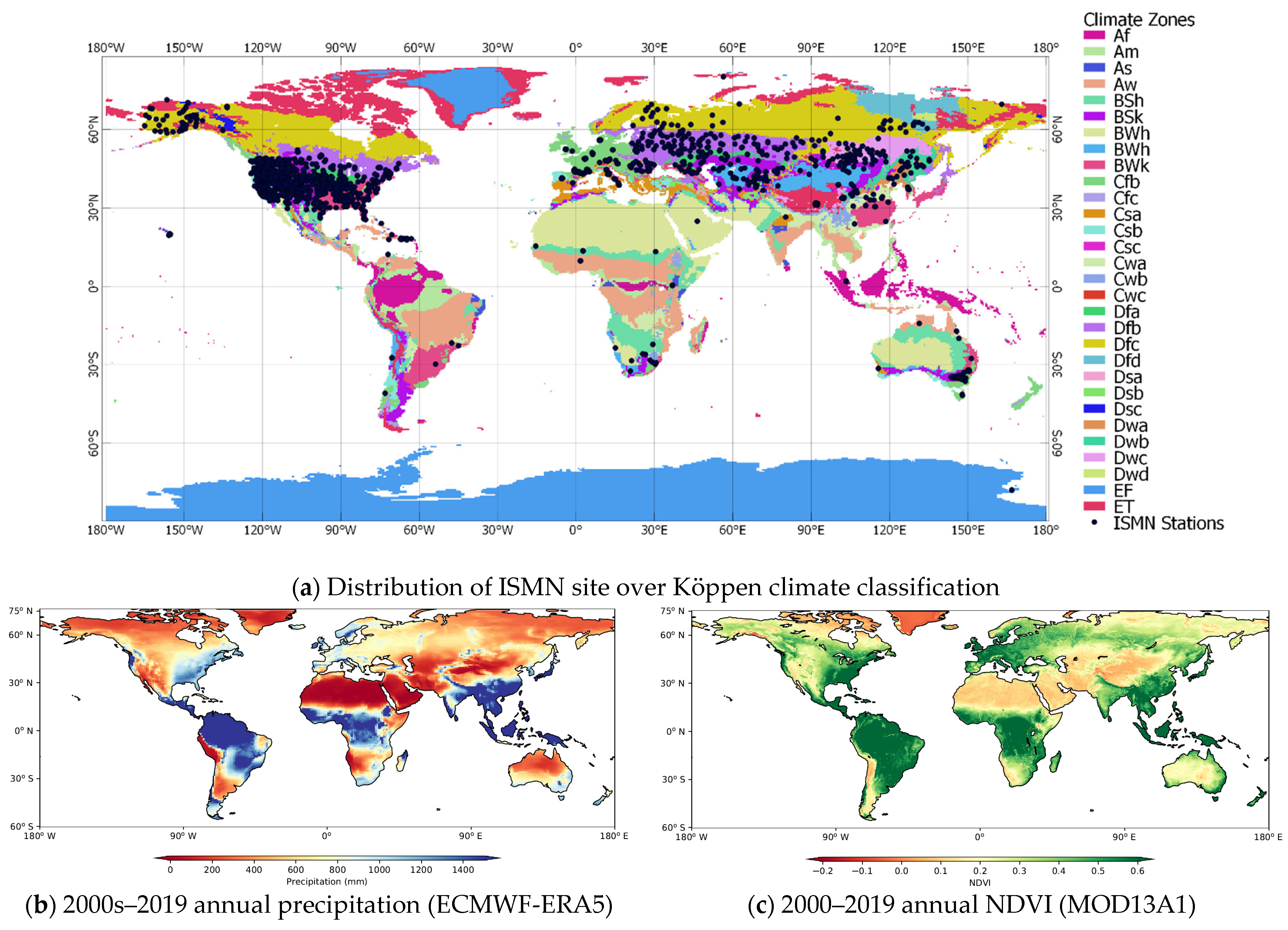
In this research, the in situ SSM data from the International Soil Moisture Network (ISMN) [31] was selected for the RF model training and validation. The ISMN was initialized to collect the in situ SM into an open-access database since 2009. By the end of 2020, the database consisted of 2678 stations from 65 networks around the world, and ISMN is still growing [8] (see network distribution in Figure 1a). The ISMN in situ data were collected from different organizations/groups; there is no standard protocol for the SM collection strategy, which results in a massive diversity between the data from various networks regarding, e.g., the sensor types installed depths, temporal measurement steps. For all these reasons, extensive efforts have been made to harmonize the in situ SM through a prime data quality control system to a reliable hourly in situ dataset [6]. The ISMN data have been widely used for the validation of SSM products from both satellites and LSMs. For example, Al-Yaari et al. (2019) assessed the reprocessed satellite-based SSM (including SMAP, SMOS, ASCAT, and ESA-CCI) using the ISMN data as the reference [32].
2.1.2. Land Surface Features and Precipitation
Many land surface features affect SSM. Table 1 summarizes the land surface features used in this study. Except for the geographical coordinates, the basic description and the source information are briefly introduced. We used Google Earth Engine (GEE) for processing most of the land surface features. With the support of the EU Copernicus Program and the agencies from the U.S. government, GEE supports direct access to petabyte-sized satellite imagery and other geospatial data. In addition, GEE provides lots of algorithms to process the data efficiently, e.g., parallel computing and machine learning [33,34] which are freely available (http://code.earthengine.google.com/, accessed on 13 September 2021).
- Land Surface Temperature
LST dominates the pattern of potential evapotranspiration and plays an essential role in SSM retrieval [35], for example, the GOES-8 satellite imager derived LST increases with the decrease of observed SSM [36]. Furthermore, the daily LST difference is related to the thermal inertia of soil with a negative relationship, while thermal inertia increases with soil moisture increase [8,37]. Thus, the daily LST difference between daytime and nighttime was also selected as a predictor variable.
Currently, several LST datasets have been produced with rigorous validations. MOD11A1 (Collection 6) LST product from Moderate Resolution Imaging Spectroradiometer (MODIS) is based on the split-window method [38,39]. The spatial resolution of the MOD11A1 is 1 km, with two measurements of LST per day: descending at local time 10:30, and ascending at 22:30, respectively. The MOD11A1 LST was reported within the average error of around 1 degree Celsius [38,40].
- Vegetation Index
The vegetation index is the reflectance transformation of two or more spectral bands from satellite imageries. For example, the Normalized Difference Vegetation Index (NDVI) is one of the most used vegetation indexes, representing the greenness of the vegetation condition, and is considered as a conservative water stress index [41]. Plenty of research has been done on retrieving SSM with the help of vegetation indices, Patel et al. (2008) proposed that Temperature/Vegetation Dryness Index (TVDI) has a strong negative relationship with the SSM [42]. Zhao et al. (2017) estimated SSM with a random forest model using LST, albedo, and NDVI [43]. In addition, the Enhanced Vegetation Index (EVI) is also commonly used to improve the sensitivity of SSM estimation at high vegetation-covered areas [44,45]. This study deployed the MOD13A1 dataset of NDVI and EVI from MODIS as the predictor variable [46]. MOD13A1 has a spatial resolution of 500 m and the temporal resolution of 16 days. The selected temporal coverage is the same as LST (from 2000 to 2019).
- Soil Texture
Soil texture heterogeneity is one of the factors that cause the spatial variability of SSM [47]. This study selected the SoilGrids soil texture data. The SoilGrids is currently the most detailed global soil dataset with a 250 m spatial resolution. It provides information on the most important soil chemical and physical properties at seven different depths: 0, 5, 15, 30, 60, 100, and 200 cm, through the ML approach [48,49,50]. Here, only the particle size distribution (sand, silt, and clay content) of the top layers (i.e., 0 cm and 5 cm) were considered because our interest was mainly focused on the land surface processes.
- Precipitation
As the primary meteorological forcing, precipitation controls SSM spatial variability in most flat areas [51,52]. Precipitation is indispensable for understanding SSM dynamics. Many studies have attempted to connect the SSM with the precipitation, for example, with the linear stochastic partial differential model [51] and Antecedent Precipitation Index (API) [53].
This study used the daily precipitation data from ERA5, which is aggregated from the 3-hourly data products [54] with a time coverage from 1978 till the present. ERA5 is one of the most advanced reanalysis products released by the European Centre for Medium-Range Weather Forecasts (ECMWF), with higher spatial resolution and better global water balance than ERA-Interim [55]. The data from 2000 to 2019 were used for synchronizing the temporal coverages of the LST and Vegetation Indices.
2.1.3. ESA-CCI SSM
The ESA-CCI SSM products [16,56,57] were selected to have a spatio-temporal comparison with the RF predicted SSM since ESA-CCI SSM is a product by blending most of the available satellite (both active and passive) SSM products (e.g., Soil Moisture and Ocean Salinity (SMOS), Advanced Microwave Scanning Radiometer for EOS (AMSR-E), Advanced SCATterometer (ASCAT)). This study used the SSM data of ESA-CCI combined version 04.4, with the temporal coverage from 1 January 2000 to 30 June 2018.
2.2. Methodology
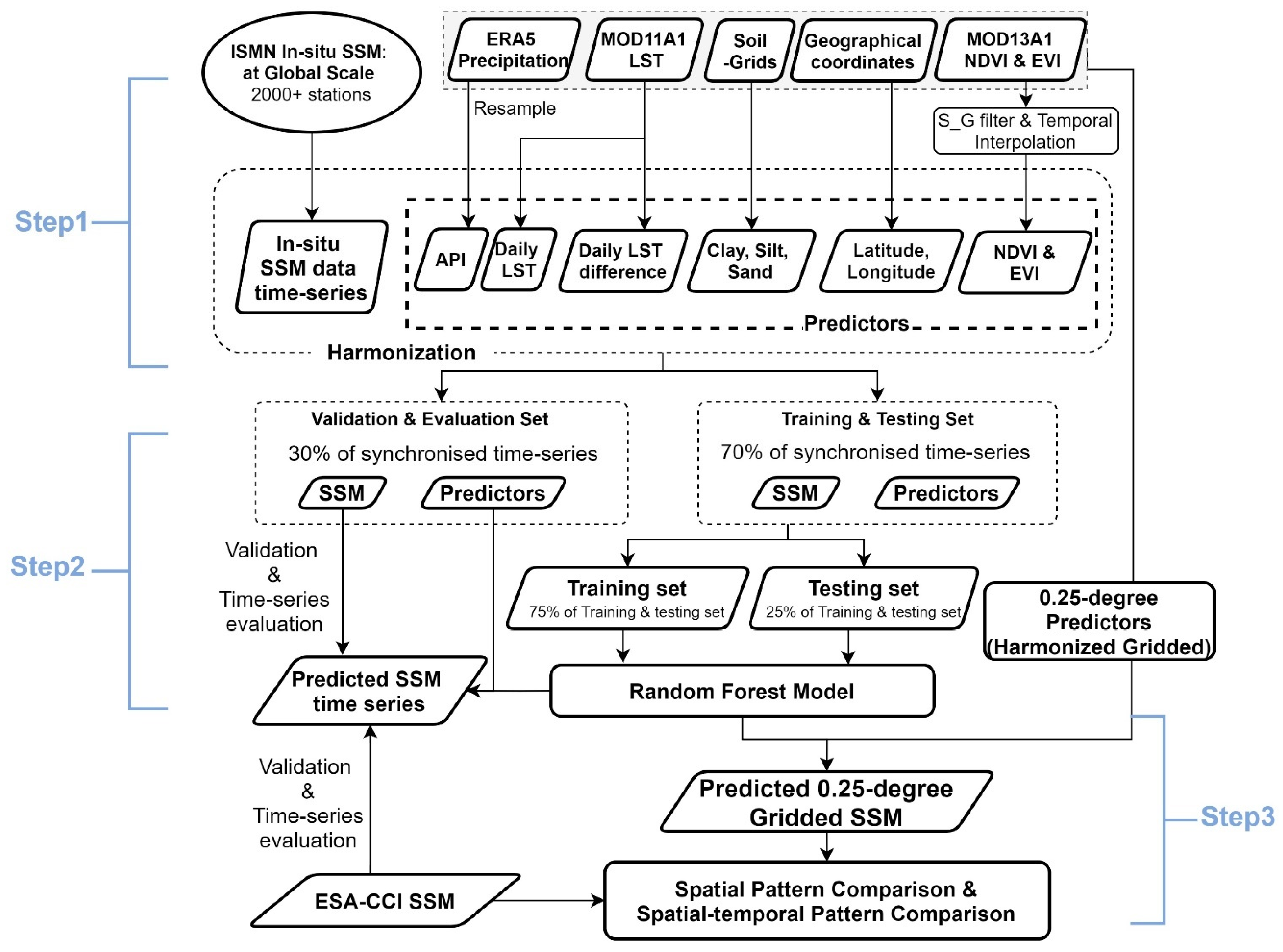
The processing methodology in this research consists of three parts: (1) data pre-processing and harmonization, (2) training and validation of the prediction model, (3) gridded SSM prediction and evaluation. See flowchart in Figure 2.
- Step 1 Data Pre-processing and Harmonization
In Step 1, we first collect in situ surface soil moisture (ISMN) and other land surface features, including daily precipitation (ERA5), land surface temperature (MOD11A1), soil texture (SoilGrids), NDVI, and EVI (MOD13A1). Then, convert daily precipitation into Antecedent Precipitation Index (API), and apply a smooth filter on NDVI and EVI before daily interpolation. See details in Section 2.2.1.
- Step 2 Training and Validation of the Prediction Model
In Step 2, we first split the data from Step 1 into two sets (i.e., training & testing set, validation & evaluation set) with the proportion of 70% (training & testing set) and 30% (validation & evaluation set) of the whole time-series. In the training & testing set, 75% of the data is used for the RF model training, and the rest 25% is used for testing the RF model’s prediction ability. The validation & evaluation set is used to evaluate the robustness of the trained model, see details in Section 2.2.2.
- Step 3 Gridded SSM prediction and evaluation.
In Step 3, we first apply the trained RF model with gridded land surface features to calculate the long-term global surface soil moisture. Then compare the spatio-temporal pattern of the RF- predicted gridded SSM with the ESA-CCI SSM, see details in Section 2.2.3.
2.2.1. Data Pre-Processing and Harmonization
- Daily LST and Daily LST Difference
The MOD11A1 LST product consists of two LST datasets per day at 10:30 and 22:30 local time. We consider the arithmetic average of those two records as daily LST and calculate the difference between the daytime and night-time value as the Daily LST difference for that day.
Provided with the LST from both daytime and night-time, the associated quality control (QC) band was used to ensure the quality of the LST (Wan, 2014). Only the pixels with the QC band value of 0 (i.e., good quality data) were kept. The MOD11A1 data used in this study starts from 24 February 2000 to 31 December 2019.
- Vegetation Index Reconstruction
Both NDVI and EVI from MOD13A1 are MODIS 16-days’ composite data. Despite an atmospheric correction procedure for the MODIS reflectance data, noise could still be observed in the long-term time series, which is not reasonable based on plant phenology. Thus, we apply the Savitzky–Golay (S-G) filtering method to reduce the small peak noise through a smoothing procedure [58]. And we also interpolated NDVI/EVI to a daily temporal step using a simple linear approach to synchronize the temporal steps with other features, see the equation below.
where p(t) is the interpolated value, and are the value at time t0 and t1, respectively.
- Antecedent Precipitation Index
The ERA5 daily precipitation data was used to calculate the Antecedent Precipitation Index (API) with Equation (2). API indicates the reverse-time-weighted summation of precipitation over a specified time [59]. The historical precipitation influence the soil water content in a weakening effect along the reverse time axis; the more recent rainfall event has the higher impact on the current SSM [60]. Many researchers applied API to retrieve SSM information [59,61]. Here we use the API as a feature for the SSM prediction. The definition of API at day t can also be represented as the equation below:
where is an empirical factor (decay parameter) to indicate the decay effect from the rainfall, which should always be less than one, a suggested range of k is between 0.85 and 0.98 [62], where is the API value at day of t, and is the precipitation value at th day before the day of t.
Despite the spatial heterogeneity of decay parameter (k), since the soil water retention varies from space, most researchers use only one pair of values (k and t) for their study area [63], which is adopted in this study as well. Here, we calculated the API with different combinations of the parameters (k and t) and compared the API and in situ SSM with Pearson Correlation Coefficient (r), and we chose the optimized parameters (k is 0.91 and t is 34).
- Spatial Resampling
Land surface features have different spatial resolutions. The land surface feature was extracted from their original resolution for pixels that collocate with the in situ site in RF model training. It is 0.25 degrees for the API, 500 m for NDVI and EVI, 1 km for LST, and 250 m for soil grids. For calculating the long-term gridded global SSM, the land surface features were aggregated into 0.25 degrees resolution, which is around 27,830 m at the equator. The World Geodetic System of 1984 (EPSG:4326) was chosen as the geographic coordinate system in our study.
- Data splitting
The API, daily LST, daily LST difference, and NDVI/EVI data were synchronized based on the temporal coverage of in situ data time-series of each ISMN station. Here is the strategy of data split: First, divide the predictors and SSM into training & testing set (70%) and validation & evaluation set (30%) based on the time series. For example, assuming the data were recorded from 1 January 2000 to 31 December 2019, the training & testing set consists of the first 70% data (14 years, from 2000 to 2013), and the validation & evaluation set consists of the last 30% data (6 years, from 2014 to 2019). Second, split the training & testing set into two parts (e.g., training set and testing set) randomly with the proportion of 75% and 25% (in RF algorithm).
2.2.2. Training and Validation of RF Model
Random Forest (RF) is an ensemble learning method that outputs a result based on many individual training models (trees). RF follows the Bootstrap Aggregation (Bagging) strategies, i.e., random sampling with replacement [64].
Given a training set of with the related predictors of , RF randomly chooses samples with replacement to form the subset of the original training set as , . The following Equation (3) explains the relationship between and , where express the relationship.
when repeating the equation with N times (i.e., building N trees), the predicted output would be expressed according to the following Equation (4):
The model testing and validation were evaluated based on the comparison of predicted and in situ SSM with several commonly used statistical metrics, including Root Mean Square Error (RMSE, Equation (5)), unbiased Root Mean Square Error (ubRMSE, Equation (8), Pearson Correlation Coefficient (r, Equation (6)), and the Mean Difference (MD, Equation (7)):
where is predicted SSM (m3 m−3), is in situ SSM (m3 m−3), N is the number of valid pairs of SSM data, is the mean value of the predicted SSM data (m3 m−3). Furthermore, RF SSM and in situ SSM of validation and evaluation set were plotted together in time-series to have a direct comparison.
To interpret the results, impurity-based feature importance and partial dependence plot were computed to better understand how the land surface features affect the SSM. All the statistical analyses were performed in the Scikit-learn package in Python [65]. The feature importance is computed as a normalized total reduction in node impurity by that feature over all trees, further details of the package can be found on the website: https://scikit-learn.org/stable/ (accessed on 13 September 2021).
2.2.3. Gridded SSM Prediction and Evaluation
The last step is to apply the trained RF model on the 0.25 degrees resolution gridded land surface features to predict the long-term gridded SSM at the global scale. And compare the RF-model Predicted gridded SSM (at 0.25 degrees) with ESA-CCI SSM products. A large quantity of the in situ SSM data originates from the continental United States. Therefore, a more detailed comparison was performed at a regional scale for that region. In addition to the simple comparison through the multiple years’ mean SSM map, we also used the Hovmöller diagram to show the longitudinal and latitudinal temporal variability.
3. Results and Discussion
The results consist of training and testing of the RF model, the feature importance, partial dependence plot, and the evaluation of the robustness of the model with statistical metrics and the time-series comparison.
3.1. Training and Testing of the Prediction Model
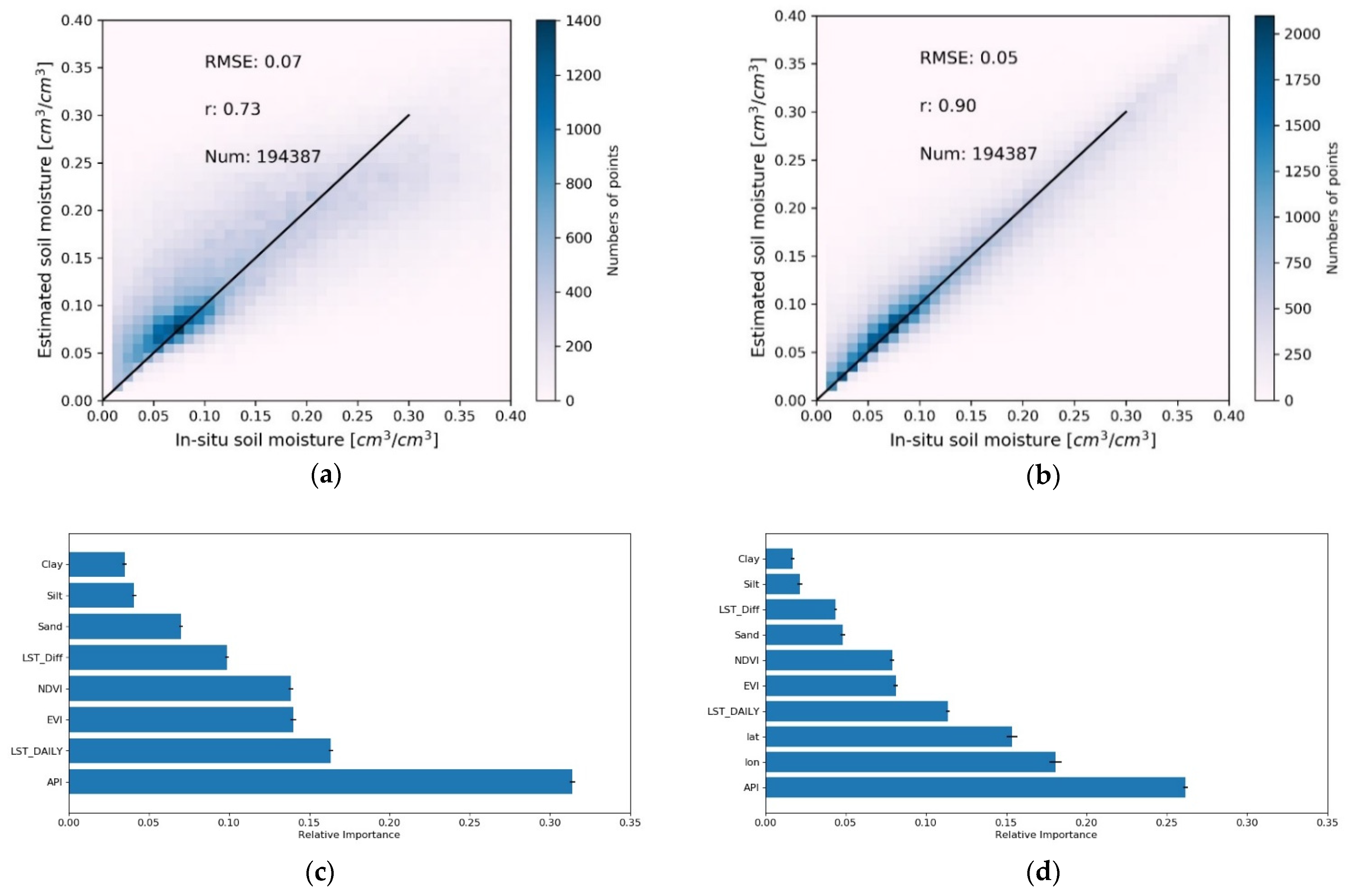
In situ SSM from 2206 stations was selected in this study, with their data extent are longer than one year. The RF model was trained using the training set with one thousand trees. Then this model was applied to the testing set to predict the SSM. Two independent pieces of training were implemented, one model was trained with all the land surface features except geographical coordinates (Model I), and one was trained with all the land surface features (Model II).
Figure 3a,b show the scatterplot of predicted and in situ SSM based on 194,387 samples of the testing set. As presented in Figure 3a (Model I), the results are quite satisfactory with RMSE of 0.07 (m3 m−3), ubRMSE of 0.07 (m3 m−3), and r of 0.73. If the geographical coordinates were included in the model (Model II), the prediction performance improved to an RMSE of 0.05 (m3 m−3), ubRMSE of 0.05 (m3 m−3), and r of 0.90, as shown in Figure 3b. Figure 3c indicates that the dominant features (predictors) in Model I are API and the daily LST. Then EVI and NDVI show similar importance. The followed less important features are daily LST difference and soil texture information. In Model II, the geographical coordinates show a high importance level, being the second and third most important variables (see Figure 3d).
3.2. Predicted SSM Time-Series of Validation and Evaluation Set
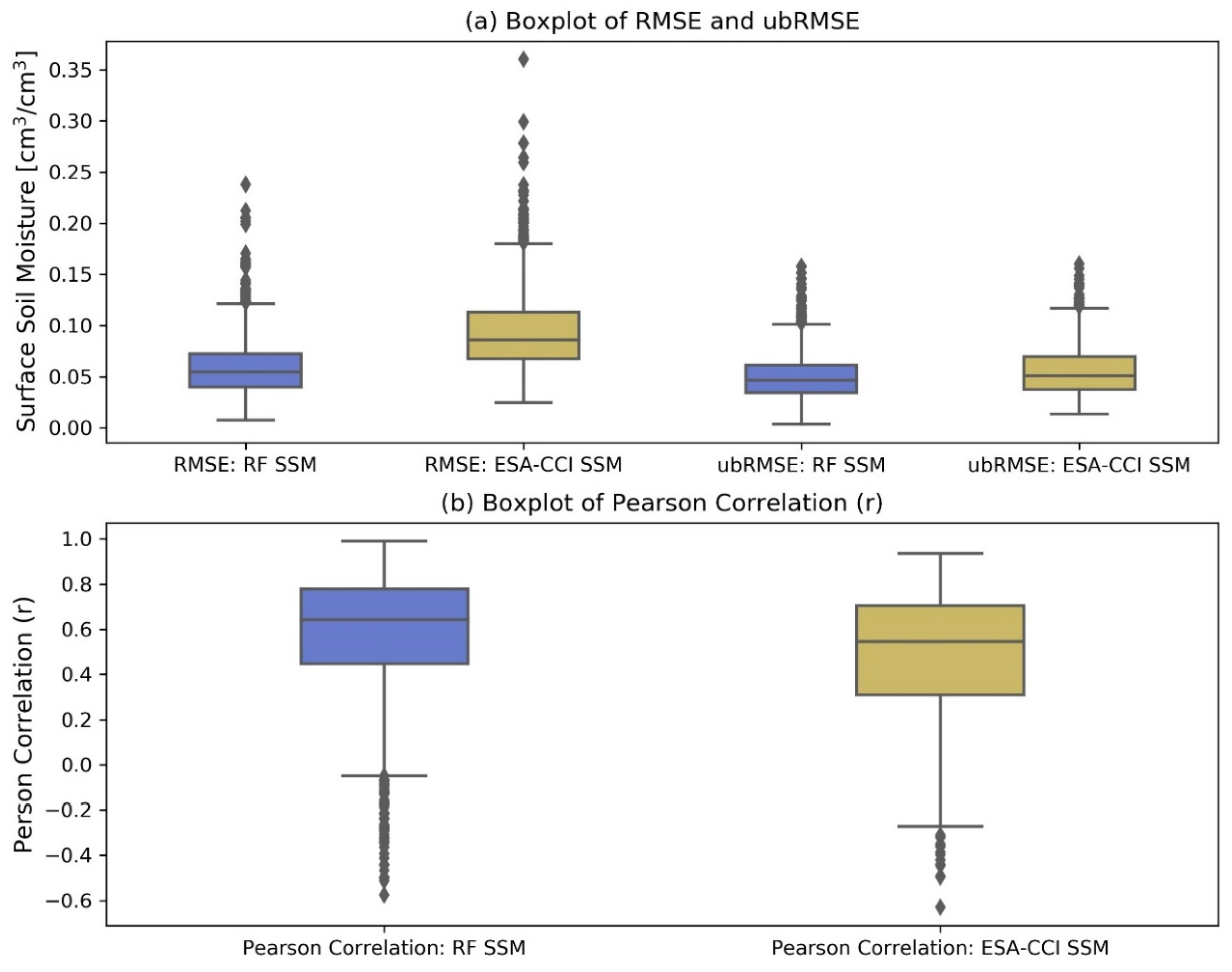
The trained model II was then applied to the validation datasets that are distributed around the world. Figure 4 shows boxplots of statistical metrics of the validation period, together with a comparison with ESA CCI SSM. The median of RMSE and ubRMSE for all stations is 0.052 (m3 m−3and 0.045 (m3 m−3), and the median r value is 0.65. ESA-CCI SSM shows a median of RMSE and ubRMSE of 0.080 (m3 m−3) and 0.055 (m3 m−3) and the median r of 0.55, respectively. The performance of the presented method is satisfactory and in line with the literature, e.g., Shen et al., 2016 evaluated the ESA-CCI v02 SSM over China with 547 stations in situ data, with the median r of 0.368, and ubRMSE of 0.069 m3 m−3 [66]; Albergel et al., 2012 evaluate ASCAT, SMOS and ECMWF soil moisture analysis (SM-DAS-2) over Africa, Australia, Europe and the United States with more than 200 stations, and the average RMSE is larger than 0.178 m3 m−3 [9].
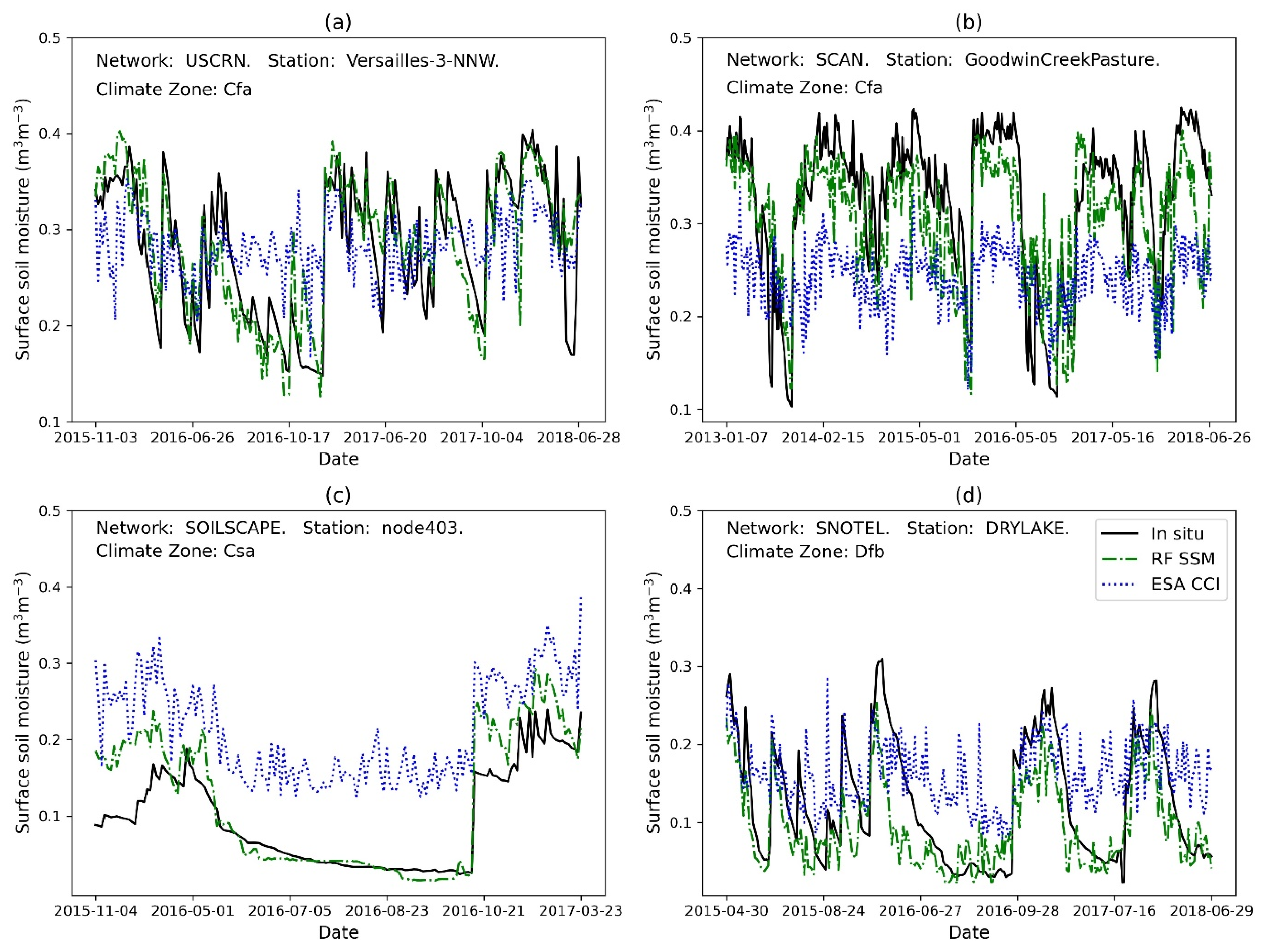
The predicted SSM and ESA CCI SSM time-series have been plotted along with the in situ SSM to evaluate the performance of temporal variability of predicted SSM. Figure 5a shows the comparison at the station Versailles-3-NNW, in the humid subtropical zone (Cfa) and covered with grassland. Both the RF SSM and ESA-CCI SSM capture the annual or interannual variabilities reasonably well, and RF SSM could predict some detailed information in the spring and autumn. In other stations, the RF SSM overperforms ESA-CCI SSM, e.g., the station GoodWinCreekPasture of SCAN in Figure 5b, the station node403 of SoilSCAPE in Figure 5c, and the station DryLake of SNOTEL in Figure 5d, covering various climate zones (humid subtropical zone (Cfa), hot-summer Mediterranean climate (Csa), humid continental climate (Dfb).
3.3. Global Scale Comparison
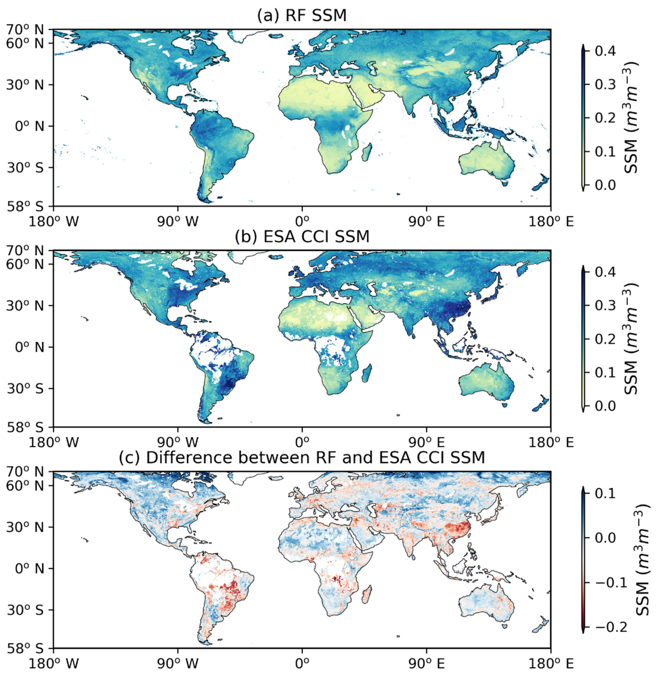
Figure 6 shows the annual mean value of the RF-predicted and ESA-CCI SSM of 2015. A similar spatial pattern is observed between Figure 6a,b, although the RF-model predicted SSM (hereafter as RF SSM) seems smoother than ESA-CCI SSM. Figure 6c depicts that the RF SSM is relatively lower than ESA-CCI SSM at wetter region and higher value at the drier region, for example, in south-eastern China, the RF SSM is 0.2 m3 m−3 lower than the ESA-CCI SSM, while in the western U.S. and western Australia, RF SSM is 0.1 m3 m−3 higher than ESA-CCI SSM.
In addition, the RF SSM map includes the SSM information in the northern part of South America, the middle part of Africa, and Indonesia. Those regions are the tropical rainforest, which has been masked out in the ESA-CCI SSM products due to the signal scattering and attenuation of the vegetation [56].
3.4. Regional Scale Comparison
3.4.1. Spatial Patterns
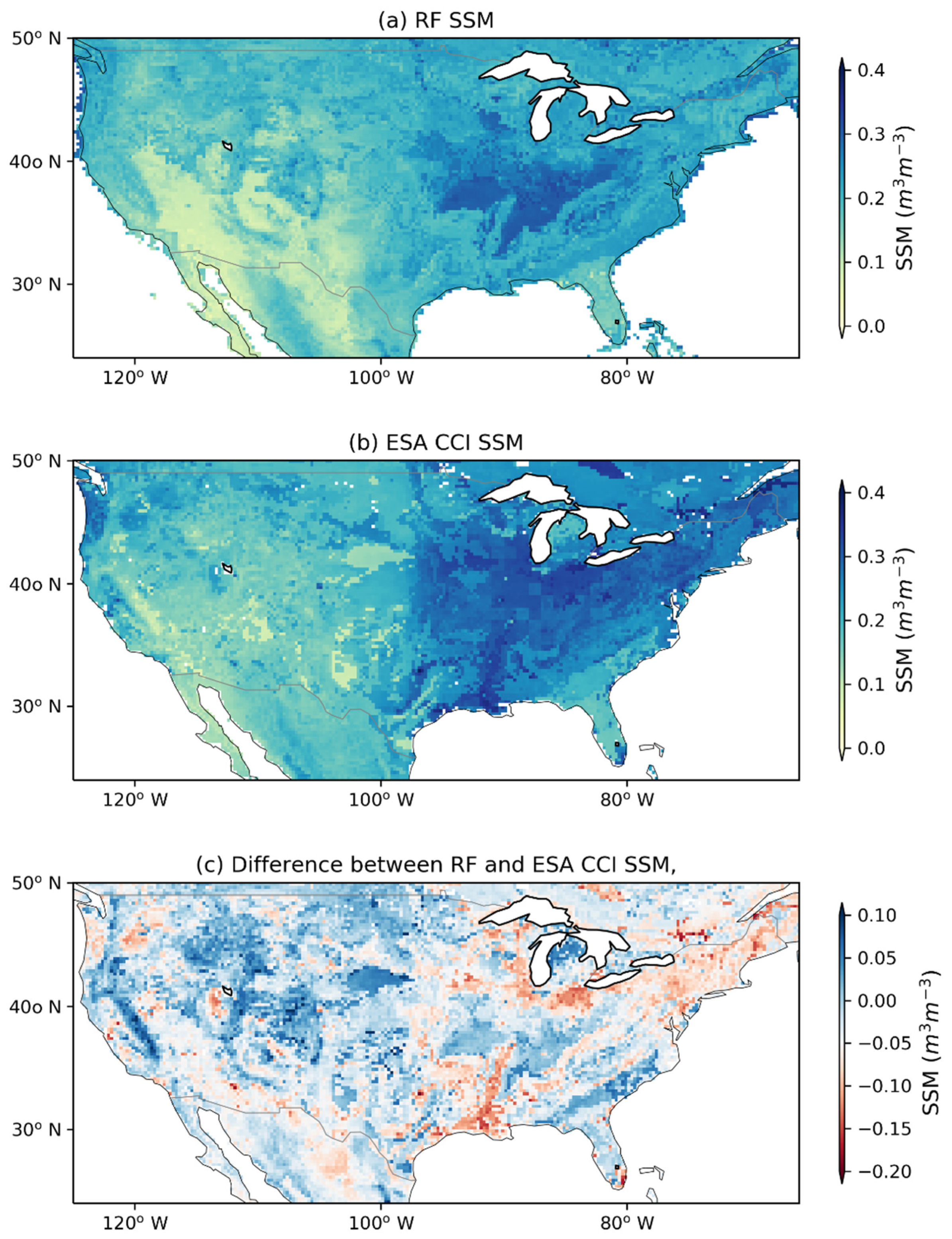
Figure 7a,b shows the average RF SSM and ESA-CCI SSM from 24 February 2000 to 30 June 2018 over the continental United States.
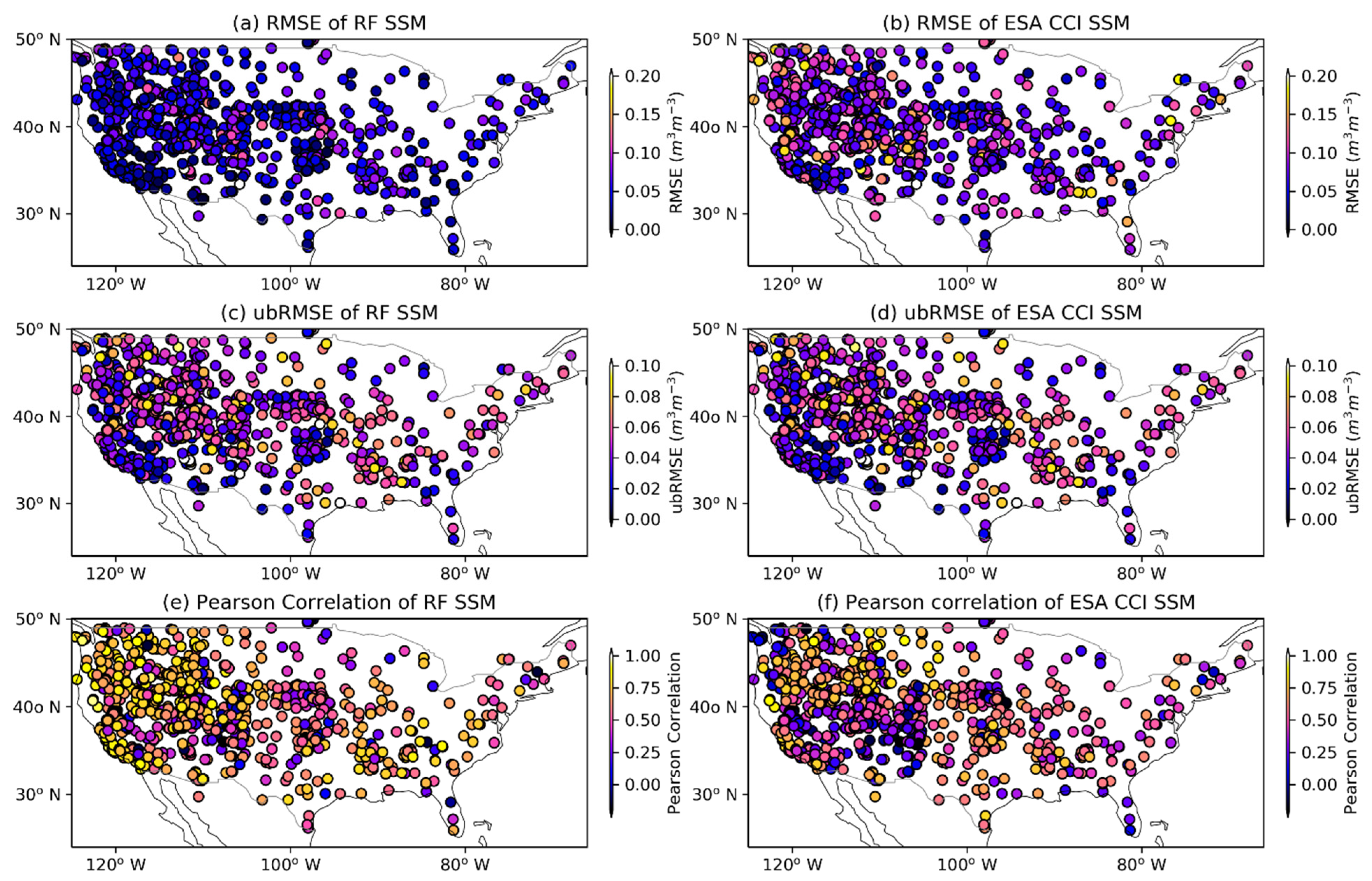
In general, the two SSM maps (Figure 7a,b) show a similar spatial pattern: a relatively dry condition in the southern part and some discrete wet regions in the northern part of the west coast. A humid region was observed in the east side of the U.S., while towards the southeast (close to Florida), the soil becomes drier again. The general spatial pattern of the difference between the RF model predicted and ESA-CCI SSM is shown in Figure 7c. Figure 8 shows the distribution maps of statistical metrics of these two products with the in situ measurements as the reference. To make it comparable, the same evaluation period is used for ESA-CCI SSM and RF SSM.
In general, RF SSM shows a relatively low value of errors, especially for the coastal area and mid-western part of the continent (Figure 8a–d). Also, when comparing the Pearson Correlation of the two products (Figure 8e–f), a significantly higher r can be found in RF SSM for these regions. Furthermore, the difference between RMSE and ubRMSE is less significant in the RF SSM, which indicates a lower bias [67].
3.4.2. Spatio-Temporal Patterns
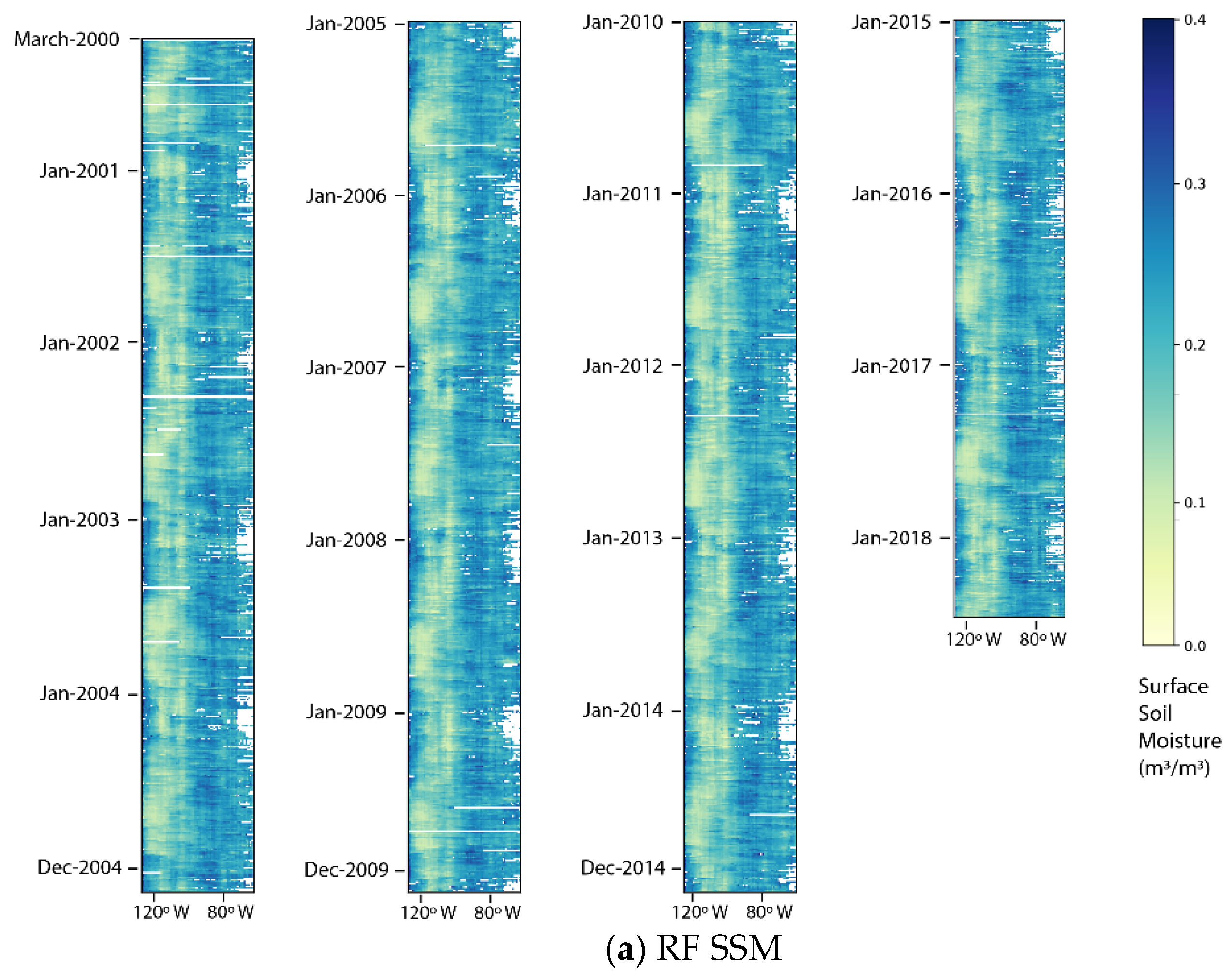
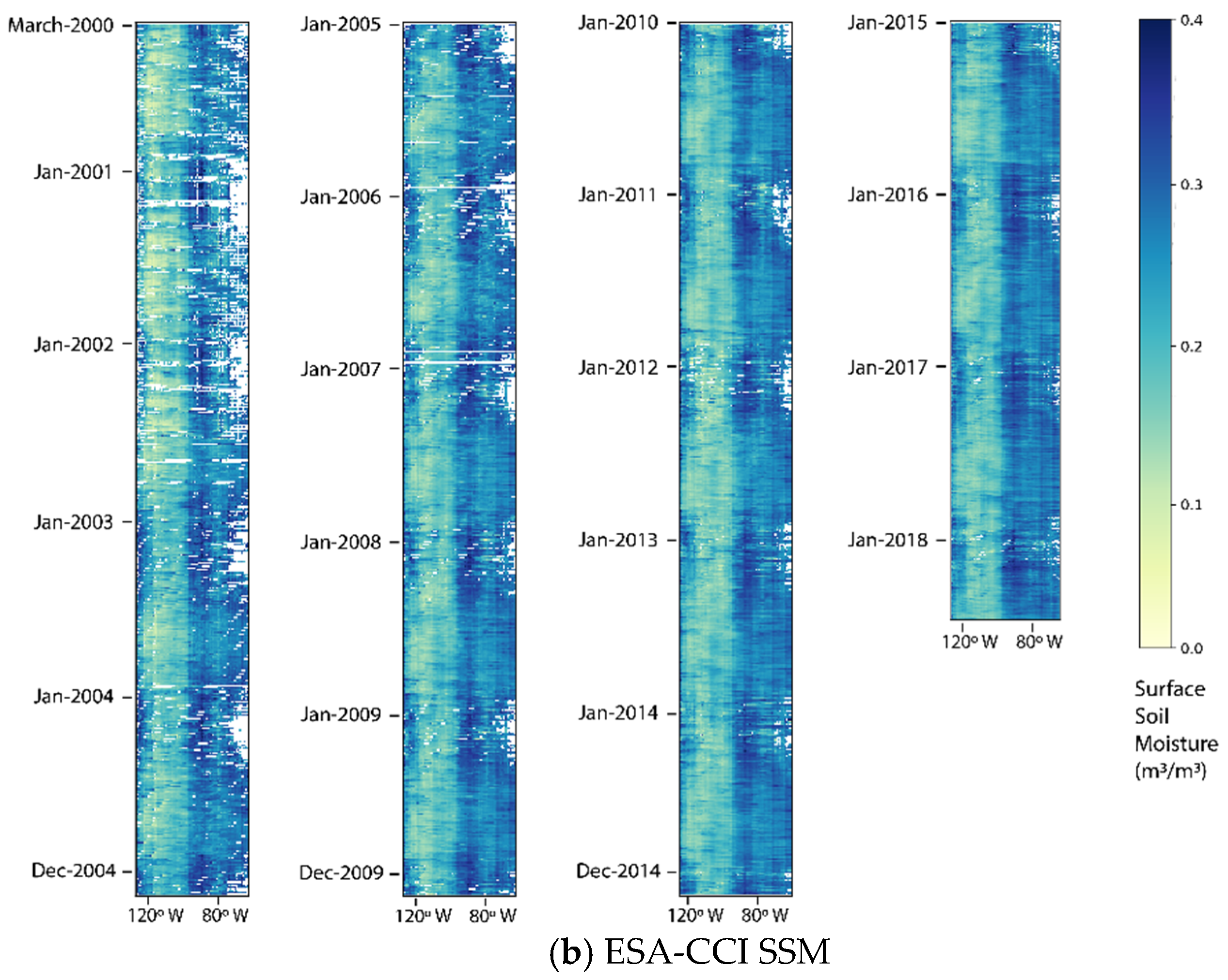
The longitudinal temporal variability of the RF SSM and ESA-CCI SSM for the continental U.S., over 24 February 2000 to 30 June 2018, is presented in Figure 9.
The pixel value of the time-longitude diagram is the average value of all the pixels along the longitude in one day. From the time axis, the seasonal and yearly variability can be observed, and along the longitude axis, the spatial distribution of SSM from west to east can be observed as well. First, the spatial pattern is evident in both RF SSM (Figure 9a) and ESA-CCI SSM (Figure 9b) that the midwestern U.S. is relatively dry and the eastern part is relatively wet. There is a significant seasonal variation on the west coast (relatively wet during winter and dry in other seasons), which matches the temporal precipitation distribution at this region. Also, in the middle eastern part, the seasonal difference is evident. Annually, some humid months appear in the central-western part, like in June 2017 and August 2017, while in 2012, it was dry. In general, ESA-CCI SSM shows higher SSM values than the RF predictions.
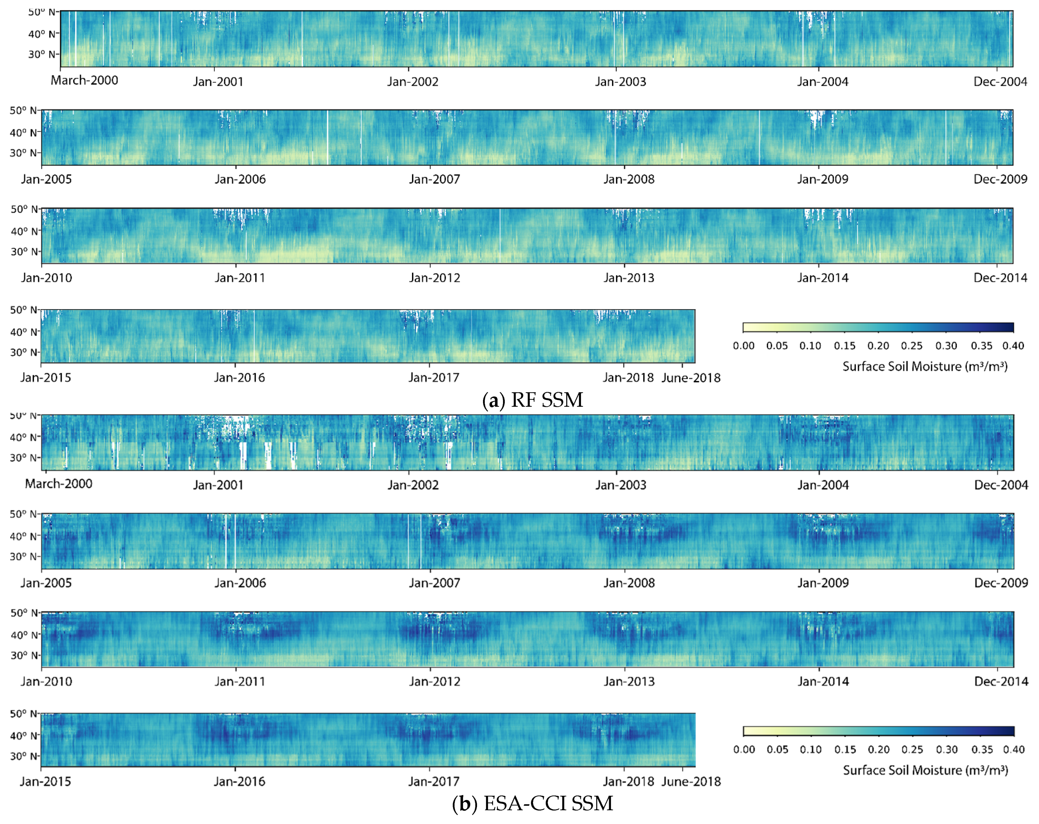
The time-latitude diagram can be used to explore the latitudinal temporal variability of the regional (the continental U.S.) data. The time-latitude diagram of the RF SSM and ESA-CCI SSM for about 18 years are presented in Figure 10. The pixel value of the time-latitude diagram is the average value of all the pixels along that latitude on one day. From the time axis, the seasonal and yearly variability can be observed, and along the latitude axis, the spatial distribution from south to north can be seen. The spatial variabilities are evident in both RF SSM (Figure 10a) and ESA-CCI SSM products (Figure 10b): dry spring and wet autumn in the southern part and wet winter in the northern part. The annual differences are also significant, such as the wet year in 2012 and the relatively dry year in 2014.
3.5. Influence of Predictor Variables
The land surface features used in this research include daily dynamic features and static features. The dynamic features consist of daily LST, daily LST difference, NDVI/EVI data from satellites data, and API from reanalysis products, helping capture the spatial-temporal variability of SSM. The static features (soil texture and geographical coordinates) also influence spatial variability. Both features are crucial in predicting the SSM through the RF model Figure 3 and Figure 11).
API is the most crucial dynamic feature with the highest importance value in the RF model, and the predicted SSM increases with the increase of the API. NDVI/EVI has a significant seasonal dynamic but a less annual variation. LST show not only annual and seasonal dynamics but also considerable daily and inter-daily dynamics. The RF model provides a possibility to capture all these intertwined features in a highly nonlinear manner.
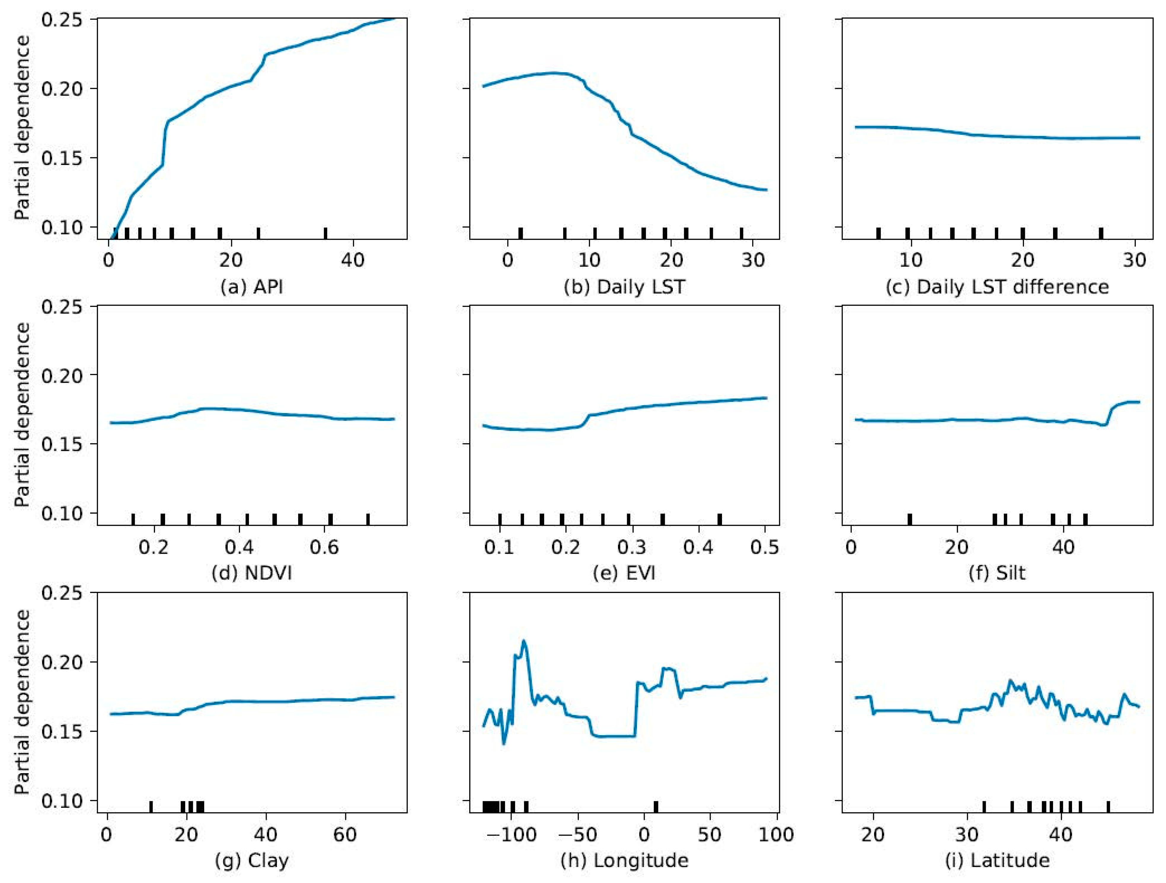
Figure 11a shows that the SSM increases with the increase of API in a strong positive relationship. Figure 11b depicts daily LST does not affect the SSM when lower than 7 degrees Celsius, and with the increase of daily LST higher than 7 degrees Celsius, SSM decreased. A relatively steady trend is observed in Figure 11c–g, which are the features with less importance shown in Figure 3. It is noted that the fluctuated trend observed in Figure 11h,i, that both the longitude and latitude have an accountable and complex effect on the SSM.
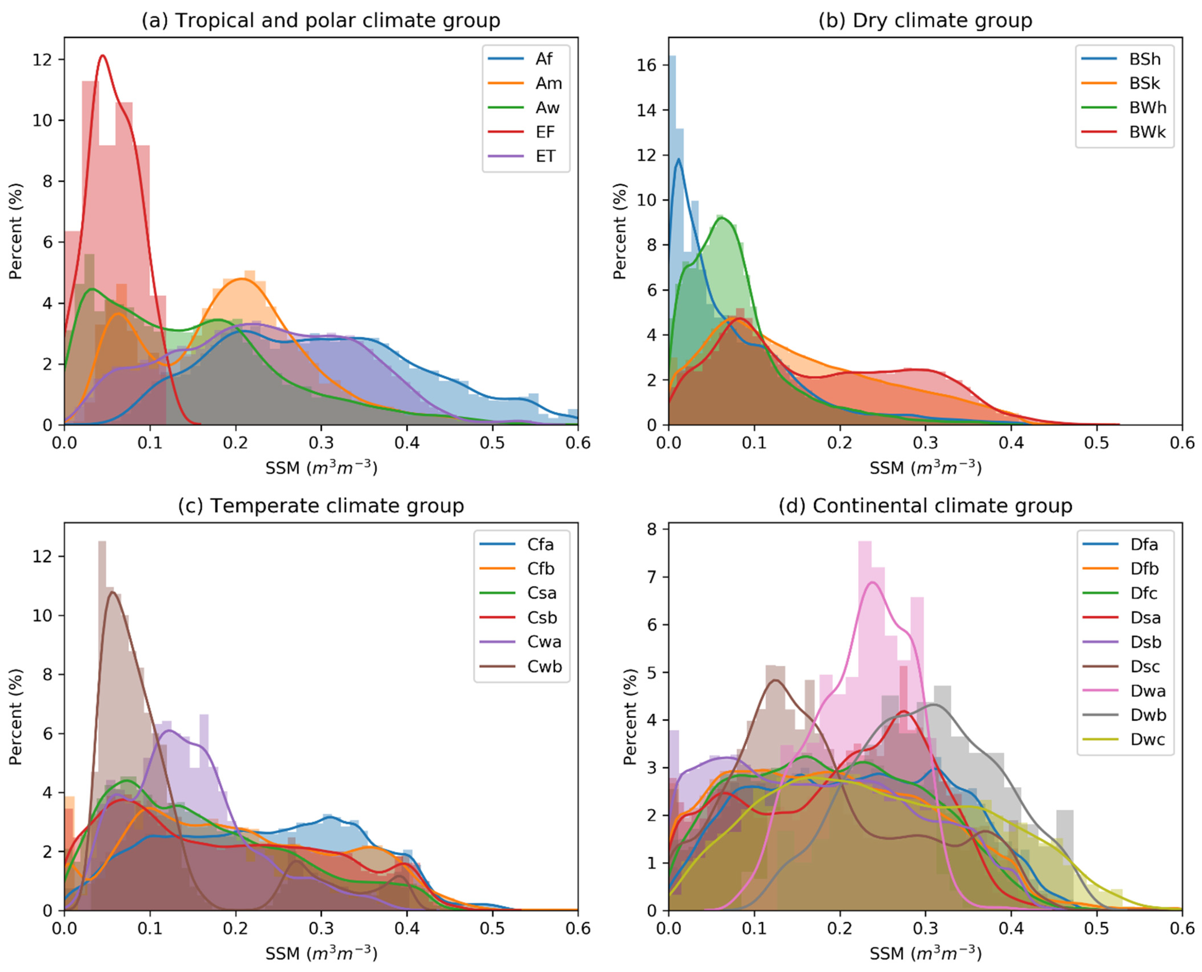
The model’s performance improves significantly with the geographical coordinates (i.e., Model I vs. Model II in Figure 3). The main reason is that the location information could be linked with the spatial distribution of the climate zones. The latitude determines the solar radiation and the longitude related to the closeness to the oceans (moisture and temperature). It can be found in Figure 3 that the longitude has higher importance than the latitude since the climate zones along the longitude are more distinct than along the latitude in the case of the training data used to build the RF model. The spatial characteristic of the annual SSM average corresponds to the spatial distribution of the climate zones, which can be further illustrated using the frequency distribution (Figure 12) of in situ SSM in each climate zone (Figure 1a).
Figure 12 shows the frequency distribution of SSM in each climate zone. A Peak to the left can be observed in some climate zones (e.g., EF in Figure 12a, Bwh and Bsh in Figure 12b, Cwb in Figure 12c). Also, a distribution close to normal distribution can be found, especially in the continental climate group (Dwa and Dwb in Figure 12d). In a word, the SSM varies a lot in different climate zones, which makes the geographical coordinates important in SSM prediction.
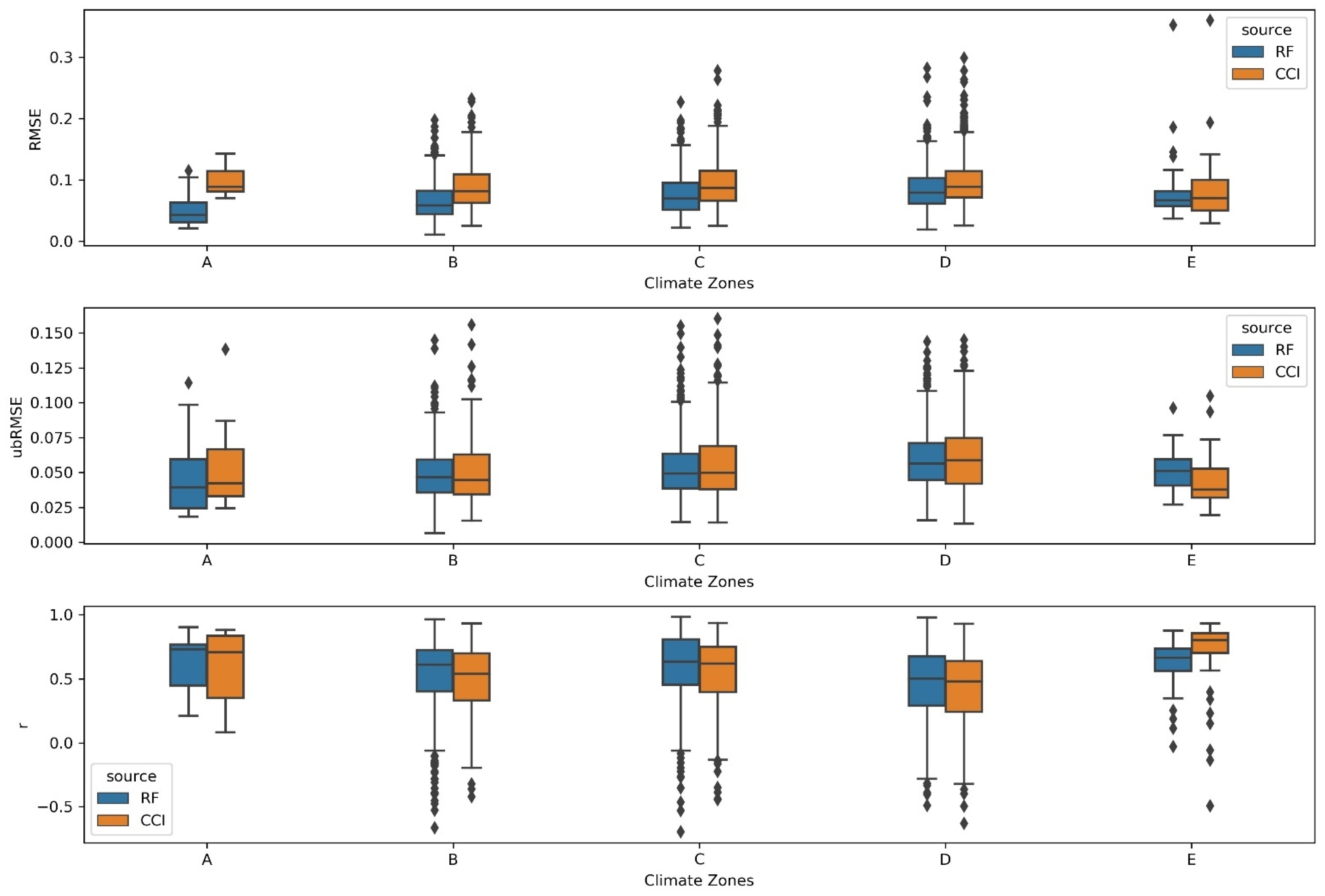
Figure 13 shows both RF SSM and ESA-CCI SSM perform well at different climate zones. RF model predicted SSM shows a relatively poorer result than ESA-CCI in the Polar climate, where most of the polar climate in situ data are from the Tibetan Plateau [8]. The passable performance of our model at polar climate might be due to the limitation of land surface feature accuracy at the Tibetan Plateau. While ESA-CCI SSM has a relatively higher RMSE in the tropical climate zones, this is due to the strong signal scattering on the vegetation [56].
4. Conclusions
This study generated a long-term in situ based gridded SSM dataset: SSM prediction was derived with RF model trained on the in situ SSM and corresponding land surface (atmospheric) properties (e.g., API, daily LST, daily LST difference, NDVI/EVI, soil texture, geographical coordinates) at the global scale. In general, the trained RF model shows a satisfactory performance compared to in situ measurements. The testing results show an RMSE of 0.05 m3 m−3, ubRMSE of 0.05 m3 m−3, and Pearson Correlation Coefficient (r) of 0.9. The evaluation results of the RF model at in situ stations also show satisfactory performance with the median of the RMSE and ubRMSE of 0.052 m3 m−3and 0.045 m3 m−3, respectively.
The spatial pattern of the predicted SSM was compared with the ESA-CCI SSM. Both products show an excellent description of the spatial variability of SSM at the global scale. At the regional scale (the U.S.), both SSM products show a similar spatial pattern in general, although some details are different in the two products. Based on the spatial distribution maps of statistical metrics of RF SSM and ESA-CCI SSM, both products can similarly perform well. RF SSM has a generally lower RMSE, a lower difference between RMSE and ubRMSE, and a higher r. The RF SSM shows a similar spatio-temporal pattern with the ESA-CCI SSM based on the longitudinal and latitudinal time-series diagram; both capture temporal variety at the scale of daily, seasonal, and annual variability. A systematic difference was also observed between the RF and ESA-CCI SSM. RF model predicted SSM is smoother on spatial pattern compared to ESA-CCI SSM, the RF model predicted SSM is relatively lower (higher) than ESA-CCI SSM in the wet(dry) region.
The presented error metrics are relevant for the pedoclimatic zones covered by the ISMN stations. Performance of the RF SSM in other zones requires further analyses, which is demanding due to the sporadicity of in situ SSM measurements and their data access restrictions. Overall, the trained RF model gives a satisfactory estimation with information on feature importance, which refers to a descending sequence: API, geographical coordinates, LST, VIs, LST difference, soil texture. Except for the dynamic variables, the geographical coordinates are particularly important, as the geographic location is linked to climate zones, which is related to precipitation and solar radiation that dominate the spatio-temporal patterns of SSM. It is also illustrated that the longitude is slightly more critical than the latitude for predicting SSM.
The random forest model has shown great potential for SSM estimation. The in situ constrained global gridded SSM may have important implications for the hydrological/agricultural/atmospheric model to improve the understanding of the interaction between the soil-vegetation-atmosphere at a large scale. In addition, the approach proposed in this paper can be extended to derive SSM maps at higher spatial-temporal resolution (e.g., 1 km) and also advanced to estimate root-zone soil moisture.
Author Contributions
Conceptualization, L.Z. and Y.Z.; methodology, L.Z., Y.Z., R.Z. and B.S.; software, L.Z., Y.Z. and B.S.; validation, L.Z. and Q.H.; formal analysis, L.Z. and R.Z.; investigation, L.Z., Y.Z. and Z.S.; resources, L.Z., Y.Z., R.Z., B.S. and Z.S.; data curation, L.Z. and R.Z.; writing—original draft preparation, L.Z.; writing—review and editing, L.Z., R.Z., Y.Z., B.S., S.M., Q.H. and Z.S.; visualization, L.Z., R.Z. and Q.H.; supervision, Y.Z., B.S. and Z.S.; project administration, Y.Z., Z.S. and S.M.; funding acquisition, Y.Z., Z.S. and S.M. All authors have read and agreed to the published version of the manuscript.
Funding
This work was supported in part by the ESA MOST Dragon IV Program (project: Monitoring Water and Energy Cycles at Climate Scale in the Third Pole Environment), ESA ELBARA-II/III Loan Agreement EOP-SM/2895/TC-tc, the Netherlands Organization for Scientific Research under Project ALW-GO/14-29, the Netherlands eScience Center under project ASDI.2020.026, the National Natural Science Foundation of China (grant no. 91837208, 41971033, 41675106) and the Fundamental Research Funds for the Central Universities, CHD (grant no. 300102298307). The authors would also like to thank the European Commission and Netherlands Organisation for Scientific Research (NWO) for funding, in the frame of the collaborative international consortium (iAqueduct) financed under the 2018 Joint call of the Water Works 2017 ERA-NET Cofund and COST Action CA16219 “HARMONIOUS—Harmonization of UAS techniques for agricultural and natural ecosystems monitoring”. The contribution of B. Szabó was supported by the János Bolyai Research Scholarship of the Hungarian Academy of Sciences (grant no. BO/00088/18/4) and the European Union’s Horizon 2020 research and innovation programme under grant agreement No. 862756.
Institutional Review Board Statement
Not applicable.
Informed Consent Statement
Not applicable.
Data Availability Statement
The long-term (2000–2019) in situ based gridded soil moisture data computed by the RF model is available at https://doi.org/10.6084/m9.figshare.14932884.v3 (accessed on 13 September 2021) [68]. And the script is available on the GitHub: https://github.com/Super-LeoJayZhang/Insitu_constrained_RF_SSM.git.
Conflicts of Interest
The authors declare that they have no conflict of interest.
References
- Rodríguez-Iturbe, I.; Isham, V.; Cox, D.R.; Manfreda, S.; Porporato, A. Space-time modeling of soil moisture: Stochastic rainfall forcing with heterogeneous vegetation. Water Resour. Res. 2006, 42, 1–11. [Google Scholar] [CrossRef] [Green Version]
- Wagner, W.; Lemoine, G.; Rott, H. A method for estimating soil moisture from ERS Scatterometer and soil data. Remote Sens. Environ. 1999, 70, 191–207. [Google Scholar] [CrossRef]
- Rodell, M.; Beaudoing, H.K.; L’Ecuyer, T.S.; Olson, W.S.; Famiglietti, J.S.; Houser, P.R.; Adler, R.; Bosilovich, M.G.; Clayson, C.A.; Chambers, D.; et al. The observed state of the water cycle in the early twenty-first century. J. Clim. 2015, 28, 8289–8318. [Google Scholar] [CrossRef]
- Cook, B.I.; Bonan, G.B.; Levis, S. Soil moisture feedbacks to precipitation in Southern Africa. J. Clim. 2006, 19, 4198–4206. [Google Scholar] [CrossRef] [Green Version]
- Liu, D.; Wang, G.; Mei, R.; Yu, Z.; Yu, M. Impact of initial soil moisture anomalies on climate mean and extremes over Asia. J. Geophys. Res. Atmos. 2014, 119, 529–545. [Google Scholar] [CrossRef]
- Dorigo, W.A.; Wagner, W.; Hohensinn, R.; Hahn, S.; Paulik, C.; Xaver, A.; Gruber, A.; Drusch, M.; Mecklenburg, S.; Van Oevelen, P.; et al. The International Soil Moisture Network: A data hosting facility for global in situ soil moisture measurements. Hydrol. Earth Syst. Sci. 2011, 15, 1675–1698. [Google Scholar] [CrossRef] [Green Version]
- Gruber, A.; Dorigo, W.A.; Zwieback, S.; Xaver, A.; Wagner, W. Characterizing coarse-scale representativeness of in situ soil moisture measurements from the international soil moisture network. Vadose Zone J. 2013, 12, 1–16. [Google Scholar] [CrossRef] [Green Version]
- Dorigo, W.; Himmelbauer, I.; Aberer, D.; Schremmer, L.; Petrakovic, I.; Zappa, L.; Preimesberger, W.; Xaver, A.; Annor, F.; Ardö, J.; et al. The International Soil Moisture Network: Serving Earth system science for over a decade. Hydrol. Earth Syst. Sci. 2021, 1–83. [Google Scholar] [CrossRef]
- Albergel, C.; de Rosnay, P.; Gruhier, C.; Muñoz-Sabater, J.; Hasenauer, S.; Isaksen, L.; Kerr, Y.; Wagner, W. Evaluation of remotely sensed and modelled soil moisture products using global ground-based in situ observations. Remote Sens. Environ. 2012, 118, 215–226. [Google Scholar] [CrossRef]
- Dorigo, W.A.; Gruber, A.; De Jeu, R.A.M.; Wagner, W.; Stacke, T.; Loew, A.; Albergel, C.; Brocca, L.; Chung, D.; Parinussa, R.M.; et al. Evaluation of the ESA CCI soil moisture product using ground-based observations. Remote Sens. Environ. 2015, 162, 380–395. [Google Scholar] [CrossRef]
- Bulut, B.; Tugrul Yilmaz, M.; Afshar, M.H.; ünal Şorman, A.; Yücel, I.; Cosh, M.H.; Şimşek, O. Evaluation of remotely-sensed and model-based soil moisture products according to different soil type, vegetation cover and climate regime using station-based observations over Turkey. Remote Sens. 2019, 11, 1875. [Google Scholar] [CrossRef] [Green Version]
- Brocca, L.; Melone, F.; Moramarco, T.; Morbidelli, R. Spatial-temporal variability of soil moisture and its estimation across scales. Water Resour. Res. 2010, 46, 1–14. [Google Scholar] [CrossRef]
- Chen, Y.; Yang, K.; Qin, J.; Zhao, L.; Tang, W.; Han, M. Evaluation of AMSR-E retrievals and GLDAS simulations against observations of a soil moisture network on the central Tibetan Plateau. J. Geophys. Res. Atmos. 2013, 118, 4466–4475. [Google Scholar] [CrossRef]
- Cheng, M.; Zhong, L.; Ma, Y.; Zou, M.; Ge, N.; Wang, X.; Hu, Y. A study on the assessment of multi-source satellite soil moisture products and reanalysis data for the Tibetan Plateau. Remote Sens. 2019, 11, 1196. [Google Scholar] [CrossRef] [Green Version]
- Tarek, M.; Brissette, F.; Arsenault, R. Evaluation of the ERA5 reanalysis as a potential reference dataset for hydrological modeling over North-America. Hydrol. Earth Syst. Sci. 2019, 10, 1009–1012. [Google Scholar] [CrossRef]
- Dorigo, W.; Wagner, W.; Albergel, C.; Albrecht, F.; Balsamo, G.; Brocca, L.; Chung, D.; Ertl, M.; Forkel, M.; Gruber, A.; et al. ESA CCI Soil Moisture for improved Earth system understanding: State-of-the art and future directions. Remote Sens. Environ. 2017, 203, 185–215. [Google Scholar] [CrossRef]
- Yin, J.; Zhan, X.; Liu, J. Noaa satellite soil moisture operational product system (Smops) version 3.0 generates higher accuracy blended satellite soil moisture. Remote Sens. 2020, 12, 2861. [Google Scholar] [CrossRef]
- Zeng, Y.; Su, Z.; Van Der Velde, R.; Wang, L.; Xu, K.; Wang, X.; Wen, J. Blending satellite observed, model simulated, and in situ measured soil moisture over Tibetan Plateau. Remote Sens. 2016, 8, 268. [Google Scholar] [CrossRef] [Green Version]
- Koster, R.D.; Guo, Z.; Yang, R.; Dirmeyer, P.A.; Mitchell, K.; Puma, M.J. On the nature of soil moisture in land surface models. J. Clim. 2009, 22, 4322–4335. [Google Scholar] [CrossRef] [Green Version]
- Naz, B.S.; Kollet, S.; Franssen, H.-J.H.; Montzka, C.; Kurtz, W. A 3 km spatially and temporally consistent European daily soil moisture reanalysis from 2000 to 2015. Sci. Data 2020, 7, 111. [Google Scholar] [CrossRef] [PubMed] [Green Version]
- Zhuang, R.; Zeng, Y.; Manfreda, S.; Su, Z. Quantifying long-term land surface and root zone soil moisture over Tibetan plateau. Remote Sens. 2020, 12, 509. [Google Scholar] [CrossRef] [Green Version]
- Su, Z.; Zeng, Y.; Romano, N.; Manfreda, S.; Francés, F.; Ben Dor, E.; Szabó, B.; Vico, G.; Nasta, P.; Zhuang, R.; et al. An integrative information aqueduct to close the gaps between satellite observation ofwater cycle and local sustainable management of water resources. Water 2020, 12, 1495. [Google Scholar] [CrossRef]
- Camps-Valls, G.; Verrelst, J.; Munoz-Mari, J.; Laparra, V.; Mateo-Jimenez, F.; Gomez-Dans, J. A survey on Gaussian processes for earth-observation data analysis: A comprehensive investigation. IEEE Geosci. Remote Sens. Mag. 2016, 4, 58–78. [Google Scholar] [CrossRef] [Green Version]
- Reichstein, M.; Camps-Valls, G.; Stevens, B.; Jung, M.; Denzler, J.; Carvalhais, N. Prabhat Deep learning and process understanding for data-driven Earth system science. Nature 2019, 566, 195–204. [Google Scholar] [CrossRef]
- Cai, Y.; Zheng, W.; Zhang, X.; Zhangzhong, L.; Xue, X. Research on soil moisture prediction model based on deep learning. PLoS ONE 2019, 14, e214508. [Google Scholar] [CrossRef]
- Ahmad, S.; Kalra, A.; Stephen, H. Estimating soil moisture using remote sensing data: A machine learning approach. Adv. Water Resour. 2010, 33, 69–80. [Google Scholar] [CrossRef]
- Chen, Y.; Feng, X.; Fu, B. An improved global remote-sensing-based surface soil moisture (RSSSM) dataset covering 2003–2018. Earth Syst. Sci. Data 2021, 13, 1–31. [Google Scholar] [CrossRef]
- Nori, H.; Jenkins, S.; Koch, P.; Caruana, R. InterpretML: A Unified Framework for Machine Learning Interpretability. arXiv 2019, arXiv:1909.09223. [Google Scholar]
- Szabó, B.; Szatmári, G.; Takács, K.; Laborczi, A.; Makó, A.; Rajkai, K.; Pásztor, L. Mapping soil hydraulic properties using random-forest-based pedotransfer functions and geostatistics. Hydrol. Earth Syst. Sci. 2019, 23, 2615–2635. [Google Scholar] [CrossRef] [Green Version]
- Menze, B.H.; Kelm, B.M.; Masuch, R.; Himmelreich, U.; Bachert, P.; Petrich, W.; Hamprecht, F.A. A comparison of random forest and its Gini importance with standard chemometric methods for the feature selection and classification of spectral data. BMC Bioinform. 2009, 10, 213. [Google Scholar] [CrossRef] [Green Version]
- Dorigo, W.; Van Oevelen, P.; Wagner, W.; Drusch, M.; Mecklenburg, S.; Robock, A.; Jackson, T. A new international network for in situ soil moisture data. Eos 2011, 92, 141–142. [Google Scholar] [CrossRef]
- Al-Yaari, A.; Wigneron, J.P.; Dorigo, W.; Colliander, A.; Pellarin, T.; Hahn, S.; Mialon, A.; Richaume, P.; Fernandez-Moran, R.; Fan, L.; et al. Assessment and inter-comparison of recently developed/reprocessed microwave satellite soil moisture products using ISMN ground-based measurements. Remote Sens. Environ. 2019, 224, 289–303. [Google Scholar] [CrossRef]
- Gorelick, N.; Hancher, M.; Dixon, M.; Ilyushchenko, S.; Thau, D.; Moore, R. Google Earth Engine: Planetary-scale geospatial analysis for everyone. Remote Sens. Environ. 2017, 202, 18–27. [Google Scholar] [CrossRef]
- Ghatasheh, N.A.; Abu-Faraj, M.M.; Faris, H. Dead sea water level and surface area monitoring using spatial data extraction from remote sensing images. Int. Rev. Comput. Softw. 2013, 8, 2892–2897. [Google Scholar] [CrossRef]
- Parinussa, R.M.; Holmes, T.R.H.; Yilmaz, M.T.; Crow, W.T. The impact of land surface temperature on soil moisture anomaly detection from passive microwave observations. Hydrol. Earth Syst. Sci. 2011, 15, 3135–3151. [Google Scholar] [CrossRef] [Green Version]
- Sun, D.; Pinker, R.T. Case study of soil moisture effect on land surface temperature retrieval. IEEE Geosci. Remote Sens. Lett. 2004, 1, 127–130. [Google Scholar] [CrossRef]
- Matsushima, D. Thermal Inertia-Based Method for Estimating Soil Moisture. In Soil Moisture; IntechOpen: London, UK, 2019; Available online: https://www.intechopen.com/chapters/62991 (accessed on 30 September 2021). [CrossRef] [Green Version]
- Wan, Z. New refinements and validation of the collection-6 MODIS land-surface temperature/emissivity product. Remote Sens. Environ. 2014, 140, 36–45. [Google Scholar] [CrossRef]
- Wan, Z.; Hook, S.; Hulley, G. MOD11A1 MODIS/Terra Land Surface Temperature/Emissivity Daily L3 Global 1 km SIN Grid V006; NASA EOSDIS Land Processes DAAC: Washington, DC, USA, 2015. [Google Scholar] [CrossRef]
- Sobrino, A.; Julien, Y.; Garc, S. Surface Temperature of the Planet Earth from Satellite Data. Remote Sens. 2020, 12, 218. [Google Scholar] [CrossRef] [Green Version]
- Goward, S.N.; Markham, B.; Dye, D.G.; Dulaney, W.; Yang, J. Normalized difference vegetation index measurements from the advanced very high resolution radiometer. Remote Sens. Environ. 1991, 35, 257–277. [Google Scholar] [CrossRef]
- Patel, N.R.; Anapashsha, R.; Kumar, S.; Saha, S.K.; Dadhwal, V.K. Assessing potential of MODIS derived temperature/vegetation condition index (TVDI) to infer soil moisture status. Int. J. Remote Sens. 2008, 30, 23–39. [Google Scholar] [CrossRef]
- Zhao, W.; Li, A.; Huang, P.; Juelin, H.; Xianming, M. Surface Soil Moisture Relationship Model Construction Based on Random Forest Method. In Proceedings of the IEEE International Geoscience and Remote Sensing Symposium (IGARSS), Fort Worth, TX, USA, 23–28 July 2017. [Google Scholar] [CrossRef]
- Jiang, Z.; Huete, A.R.; Didan, K.; Miura, T. Development of a two-band enhanced vegetation index without a blue band. Remote Sens. Environ. 2008, 112, 3833–3845. [Google Scholar] [CrossRef]
- Matsushita, B.; Yang, W.; Chen, J.; Onda, Y.; Qiu, G. Sensitivity of the Enhanced Vegetation Index (EVI) and Normalized Difference Vegetation Index (NDVI) to topographic effects: A case study in high-density cypress forest. Sensors 2007, 7, 2636–2651. [Google Scholar] [CrossRef] [PubMed] [Green Version]
- Didan, K. MOD13A1 MODIS/Terra Vegetation Indices 16-Day L3 Global 500 m SIN Grid V006 Data Set. Available online: https://lpdaac.usgs.gov/node/838 (accessed on 30 September 2021).
- Montzka, C.; Rötzer, K.; Bogena, H.R.; Sanchez, N.; Vereecken, H. A new soil moisture downscaling approach for SMAP, SMOS, and ASCAT by predicting sub-grid variability. Remote Sens. 2018, 10, 427. [Google Scholar] [CrossRef] [Green Version]
- Ross, C.W.; Prihodko, L.; Anchang, J.; Kumar, S.; Ji, W.; Hanan, N.P. HYSOGs250m, global gridded hydrologic soil groups for curve-number-based runoff modeling. Sci. Data 2018, 5, 180091. [Google Scholar] [CrossRef]
- Hengl, T.; De Jesus, J.M.; MacMillan, R.A.; Batjes, N.H.; Heuvelink, G.B.M.; Ribeiro, E.; Samuel-Rosa, A.; Kempen, B.; Leenaars, J.G.B.; Walsh, M.G.; et al. SoilGrids1km—Global soil information based on automated mapping. PLoS ONE 2014, 9, e114788. [Google Scholar] [CrossRef] [Green Version]
- Hengl, T.; Mendes de Jesus, J.; Heuvelink, G.B.M.; Ruiperez Gonzalez, M.; Kilibarda, M.; Blagotić, A. SoilGrids250m: Global gridded soil information based on machine learning. PLoS ONE 2017, 12, e0169748. [Google Scholar] [CrossRef] [Green Version]
- Pan, F.; Peters-Lidard, C.D.; Sale, M.J. An analytical method for predicting surface soil moisture from rainfall observations. Water Resour. Res. 2003, 39. [Google Scholar] [CrossRef] [Green Version]
- Wu, C.; Chen, J.M.; Pumpanen, J.; Cescatti, A.; Marcolla, B.; Blanken, P.D.; Ardö, J.; Tang, Y.; Magliulo, V.; Georgiadis, T.; et al. An underestimated role of precipitation frequency in regulating summer soil moisture. Environ. Res. Lett. 2012, 7, 024011. [Google Scholar] [CrossRef]
- Shaw, B.L.; Pielke, R.A.; Ziegler, C.L. A three-dimensional numerical simulation of a great plains dryline. Mon. Weather Rev. 1997, 125, 1489–1506. [Google Scholar] [CrossRef] [Green Version]
- Muñoz Sabater, J. ERA5-Land Hourly Data from 1981 to Present. Copernicus Climate Change Service (C3S) Climate Data Store (CDS). 2019. Available online: https://doi.org/10.24381/cds.e2161bac (accessed on 30 September 2021).
- Albergel, C.; Dutra, E.; Munier, S.; Calvet, J.C.; Munoz-Sabater, J.; De Rosnay, P.; Balsamo, G. ERA-5 and ERA-Interim driven ISBA land surface model simulations: Which one performs better. Hydrol. Earth Syst. Sci. 2018, 22, 3515–3532. [Google Scholar] [CrossRef] [Green Version]
- Gruber, A.; Scanlon, T.; Van Der Schalie, R.; Wagner, W.; Dorigo, W. Evolution of the ESA CCI Soil Moisture climate data records and their underlying merging methodology. Earth Syst. Sci. Data 2019, 11, 717–739. [Google Scholar] [CrossRef] [Green Version]
- Gruber, A.; Dorigo, W.A.; Crow, W.; Wagner, W. Triple Collocation-Based Merging of Satellite Soil Moisture Retrievals. IEEE Trans. Geosci. Remote Sens. 2017, 55, 6780–6792. [Google Scholar] [CrossRef]
- Chen, J.; Jönsson, P.; Tamura, M.; Gu, Z.; Matsushita, B.; Eklundh, L. A simple method for reconstructing a high-quality NDVI time-series data set based on the Savitzky-Golay filter. Remote Sens. Environ. 2004, 91, 332–344. [Google Scholar] [CrossRef]
- Wilke, G.D.; McFarland, M.J. Correlations between Nimbus-7 scanning multichannel microwave radiometer data and an antecedent precipitation index. J. Clim. Appl. Meteorol. 1986, 25, 227–238. [Google Scholar] [CrossRef] [Green Version]
- Benkhaled, A.; Remini, B.; Mhaiguene, M. Influence of antecedent precipitation index on the hydrograph shape. Br. Hydrol. Soc. 2004, 1, 81–87. [Google Scholar]
- Zhao, Y.; Wei, F.; Yang, H.; Jiang, Y. Discussion on using antecedent precipitation index to supplement relative soil moisture data series. Procedia Environ. Sci. 2011, 10, 1489–1495. [Google Scholar] [CrossRef] [Green Version]
- Ali, S.; Ghosh, N.C.; Singh, R. Rainfall—runoff simulation using a normalized antecedent precipitation index precipitation index. Hydrol. Sci. J. 2010, 52, 266–274. [Google Scholar] [CrossRef] [Green Version]
- Hillel, D. Encyclopedia of Soils in the Environment; Elsevier: London, UK, 2004; Volume 3, ISBN 9780080547954. [Google Scholar]
- Altman, N.; Krzywinski, M. Points of Significance: Ensemble methods: Bagging and random forests. Nat. Methods 2017, 14, 933–934. [Google Scholar] [CrossRef]
- Varoquaux, G.; Buitinck, L.; Louppe, G.; Grisel, O.; Pedregosa, F.; Mueller, A. Scikit-learn: Machine Learning in Python. J. Mach. Learn. Res. 2011, 2825–2830. [Google Scholar] [CrossRef]
- Shen, X.; An, R.; Quaye-Ballard, J.A.; Zhang, L.; Wang, Z. Evaluation of the European Space Agency Climate Change Initiative Soil Moisture Product over China Using Variance Reduction Factor. J. Am. Water Resour. Assoc. 2016, 52, 1524–1535. [Google Scholar] [CrossRef]
- Zhu, L.; Wang, H.; Tong, C.; Liu, W.; Du, B. Evaluation of ESA Active, Passive and Combined Soil Moisture Products Using Upscaled Ground Measurements. Sensors 2019, 19, 2718. [Google Scholar] [CrossRef] [PubMed] [Green Version]
- Zhang, L.; Zeng, Y.; Zhuang, R.; Manfreda, S.; Han, Q.; Su, Z.; Szabó, B. RF_global_SSM_2000-2019_0.25_degree 2021. Available online: https://doi.org/10.6084/m9.figshare.14932884.v3 (accessed on 30 September 2021).
Figure 1.
Distribution of the ISMN in situ over Köppen climate classification, annual Precipitation, and NDVI.
Figure 1.
Distribution of the ISMN in situ over Köppen climate classification, annual Precipitation, and NDVI.

Figure 2.
Flowchart of methodology to derive prediction model for SSM and derive SSM maps.

Figure 3.
Model validation and feature importance. (a,b) shows the scatterplot of predicted and in situ soil moisture based on the test set (N = 194,387) for the RF model without and with geographic coordinates. (c,d) are the feature importance.
Figure 3.
Model validation and feature importance. (a,b) shows the scatterplot of predicted and in situ soil moisture based on the test set (N = 194,387) for the RF model without and with geographic coordinates. (c,d) are the feature importance.

Figure 4.
Boxplot of the metrics of the validation & evaluation set: RF SSM vs. ESA-CCI. (a) boxplot of RMSE, ubRMSE, (b) boxplot of r, the RF model considering geographical coordinates.
Figure 4.
Boxplot of the metrics of the validation & evaluation set: RF SSM vs. ESA-CCI. (a) boxplot of RMSE, ubRMSE, (b) boxplot of r, the RF model considering geographical coordinates.

Figure 5.
Time-series of predicted SSM at selected stations across various climate zones with RF model II (considering geographical coordinates). (a) Station Versailles-3-NNW, USCRN; (b) Station GoodWinCreekPasture, SCAN; (c) Station Node403, SoilSCA, (d) Station DryLake in SNOTEL).
Figure 5.
Time-series of predicted SSM at selected stations across various climate zones with RF model II (considering geographical coordinates). (a) Station Versailles-3-NNW, USCRN; (b) Station GoodWinCreekPasture, SCAN; (c) Station Node403, SoilSCA, (d) Station DryLake in SNOTEL).

Figure 6.
Global annual mean SSM map (0.25 degree) of 2015, (a) RF model predicted SSM; (b) ESA-CCI SSM; (c) Difference between RF model and ESA-CCI SSM). Areas in white mean no data.
Figure 6.
Global annual mean SSM map (0.25 degree) of 2015, (a) RF model predicted SSM; (b) ESA-CCI SSM; (c) Difference between RF model and ESA-CCI SSM). Areas in white mean no data.

Figure 7.
Long-term mean SSM map over the Continental United States with 0.25 degrees resolution: (a) RF model predicted SSM; (b) ESA-CCI SSM, (c) Difference between RF model and ESA-CCI SSM over 2000 to 2018.
Figure 7.
Long-term mean SSM map over the Continental United States with 0.25 degrees resolution: (a) RF model predicted SSM; (b) ESA-CCI SSM, (c) Difference between RF model and ESA-CCI SSM over 2000 to 2018.

Figure 8.
Mean statistical metrics distribution of RF SSM and ESA-CCI SSM at the regional scale for the evaluation period.
Figure 8.
Mean statistical metrics distribution of RF SSM and ESA-CCI SSM at the regional scale for the evaluation period.

Figure 9.
Time-longitude diagram over the continental U.S.


Figure 10.
Time-latitude diagram over the continental U.S.

Figure 11.
Partial dependence plot of surface soil moisture on the predictor variables computed based on the RF model: (a) Antecedent Precipitation Index; (b) Daily LST; (c) Daily LST difference; (d) Normalized Difference Vegetation Index (NDVI); (e) Enhanced Vegetation Index (EVI); (f) Silt content; (g) Clay content; (h) Geographic coordinates (Longitude); (i) Geographic coordinates (Latitude).

Figure 12.
Frequency distribution of in situ SSM over various climate zones at the global scale.

Figure 13.
Comparison of SSM and ESA-CCI SSM with in situ data over different climate zones. (A) Tropical; (B) Arid; (C) Temperate; (D) Continental; (E) Polar.
Figure 13.
Comparison of SSM and ESA-CCI SSM with in situ data over different climate zones. (A) Tropical; (B) Arid; (C) Temperate; (D) Continental; (E) Polar.


Table 1.
Land Surface Features and Data Sources List.
| Name of Predictors * | Description | Source | Original Spatial Resolution | Original Temporal Resolution |
|---|---|---|---|---|
| Daily LST | The arithmetic average of LST of daytime and night-time | MOD11A1 daily LST product https://doi.org/10.5067/MODIS/MOD11A1.006 (accessed on 13 September 2021) | 1 km | Daily |
| Daily LST Difference | The difference between the LST at daytime and night-time | MOD11A1 daily LST product https://doi.org/10.5067/MODIS/MOD11A1.006 (accessed on 13 September 2021) | 1 km | Daily |
| NDVI | Interpolated daily NDVI | MOD13A1 https://doi.org/10.5067/MODIS/MOD13A1.006 (accessed on 13 September 2021) | 500 m | 16 d |
| EVI | Interpolated daily EVI | MOD13A1 https://doi.org/10.5067/MODIS/MOD13A1.006 (accessed on 13 September 2021) | 500 m | 16 d |
| API | Calculated Antecedent Precipitation Index | ERA-5 daily precipitation https://cds.climate.copernicus.eu/cdsapp#!/dataset/reanalysis-era5-single-levels?tab=overview (accessed on 13 September 2021) | 0.25° | Daily |
| Soil texture (clay, silt and sand) | ML-based global soil texture estimation | SoilGrids https://soilgrids.org/ (accessed on 13 September 2021) | 250 m | Static |
* LST: Land Surface Temperature; NDVI: Normalized Difference Vegetation Index; EVI: Enhanced Vegetation Index; API: Antecedent Precipitation Index.
Publisher’s Note: MDPI stays neutral with regard to jurisdictional claims in published maps and institutional affiliations. |
© 2021 by the authors. Licensee MDPI, Basel, Switzerland. This article is an open access article distributed under the terms and conditions of the Creative Commons Attribution (CC BY) license (https://creativecommons.org/licenses/by/4.0/).
Share and Cite
MDPI and ACS Style
Zhang, L.; Zeng, Y.; Zhuang, R.; Szabó, B.; Manfreda, S.; Han, Q.; Su, Z. In Situ Observation-Constrained Global Surface Soil Moisture Using Random Forest Model. Remote Sens. 2021, 13, 4893. https://doi.org/10.3390/rs13234893
AMA Style
Zhang L, Zeng Y, Zhuang R, Szabó B, Manfreda S, Han Q, Su Z. In Situ Observation-Constrained Global Surface Soil Moisture Using Random Forest Model. Remote Sensing. 2021; 13(23):4893. https://doi.org/10.3390/rs13234893
Chicago/Turabian StyleZhang, Lijie, Yijian Zeng, Ruodan Zhuang, Brigitta Szabó, Salvatore Manfreda, Qianqian Han, and Zhongbo Su. 2021. "In Situ Observation-Constrained Global Surface Soil Moisture Using Random Forest Model" Remote Sensing 13, no. 23: 4893. https://doi.org/10.3390/rs13234893
Note that from the first issue of 2016, this journal uses article numbers instead of page numbers. See further details here.