Urban buildings configuration and pollutant dispersion of PM 2.5 particulate to enhance air quality

Introduction

The impacts of the rapid increase of the world's population are dramatically reflected in the overexploitation and deficiency of environmental resources, severe desertification, global warming, and more particularly, pollution of the environment (Motevalian and Yeganeh, 2020). At present, the majority of the universal population inhabits city regions. By 2050, this amount is expected to increase to about 66%, essentially due to the urban expansion trends of developing nations (Randers, 2012; Pu and Yang, 2014; Hite and Seitz, 2021). About 98% of low and middle-income cities with more than 100,000 residents do not meet the World Health Organization (WHO) guidelines in air quality, based on the latest urban air quality data (Obanya et al., 2018).

Based on recent research that used a global atmospheric chemistry model, due to anthropogenic delicate particulate matter, each year 3.3 million premature mortality worldwide is associated with outdoor air pollution, and it is expected to double by 2050 (Lelieveld et al., 2015; Liu et al., 2019a; Allen et al., 2020). The results attained from the last decades demonstrated that fine particulate air pollution has adverse effects on cardiopulmonary health (Chang et al., 2015; Daiber et al., 2020). The air quality has worsened because of the ongoing works of political and social governments in the last decade, including recent displays of the global trends of urban expansion and mechanization (Sovacool et al., 2020).

In addition, the levels of pollution in the cities are accentuated by climatic factors (Liu et al., 2019b). Above all, solar radiation and thus the temperature in the area usually affects the depth of the lower layer of the troposphere, mixing surface emissions (Liu et al., 2019c). The less weak the diurnal emissions are, the shallower the mixing depth. Therefore, the impact of the temperature on acceptable particulate matter levels through convection is reduced (Li et al., 2019). Furthermore, solar radiation and temperature impact the formation and development of photochemical smog (Wang et al., 2020); simultaneously, wind speeds move air pollutant emissions to different regions. Even though the emission origins do not exist in a particular area, it can still exhibit enhanced air pollution levels due to winds from the source, which directly counts on wind speed (Sadaa and Salihb, 2017). Increased relative humidity has been determined to enhance the weight of fine particles, assisting the removal of the dry deposition m ethod, while precipitation instantly affects clean air by saturating deposition (Zhang et al., 2017; Sajani et al., 2018). Using an observation-based algorithm, Wang and Liu (2018) measured the spatial distribution of indicators addressing the humidity impact on East China. There are differences between the seasons, as different parameters affect the year due to the combination of conditions based on some research (Wang and Liu, 2018).

The complicated compounds of local emission origins and local transports of air pollutants give actual PM2.5 forecast a challenging yet essential assignment, particularly following high pollution circumstances (Xue et al., 2019). The essential air pollution element in Tehran has suspended particles of 2.5 microns. Exposure to PM2.5 has multiple short-term and long-term health impacts. In the short term, it triggers irritation in the eyes, nose, and throat, coughing, sneezing, and shortness of breath (Ganesh et al., 2018). Prolonged exposure to PM2.5 can cause permanent respiratory problems such as asthma, chronic bronchitis, and heart disease. While PM2.5 impacts everyone, people with breathing and heart problems, children, and the elderly are most sensitive to it (Ventura et al., 2019; Xue et al., 2019). A typical description of the spatial-temporal PM2.5 variable is the solution to efficient air pollution regulatory programs informing policymakers of essential anticipatory measures to counter air pollution (Chang et al., 2020). Hence, studying the emission origins and the propagation devices that create dangerous air pollution is crucial for efficiently formulating air pollution reduction plans (Ganesh et al., 2018; Ventura et al., 2019).

Still, only a few studies on block typology's impact on air quality exist (Ganesh et al., 2018; Ventura et al., 2019; Xue et al., 2019; Chang et al., 2020) as part of a central urban planning component. These investigations have emphasized the significance of accurately describing urban geometry. Nevertheless, most urban quality investigations utilize an idealistic pattern (Sun and Sun, 2017; Cihan et al., 2021), usually designed by square blocks uniformly spaced. Nevertheless, Yanlai et al. (2019) indicated that block typology simplification could create a utopian or impractical city. In contrast, actual urban areas are highly heterogeneous, with a vast range of mass and categorizations in similar towns. Accordingly, a block typology system can describe an intermediate approach between analyzing existing cities and simulation situations.

Statistical models, chemical transport, and machine learning are three effective methods for forecasting PM2.5 concentrations (Xue et al., 2019). A machine learning strategy can analyze different models' features compared to an ineffective statistical model (Chang et al., 2020). Artificial Neural Networks are the best-known classifiers for predicting pollution levels (Ganesh et al., 2018; Ventura et al., 2019). Several artificial intelligence algorithms, such as fuzzy logic and artificial neural network (ANN) (Cihan et al., 2021), or Principal Component Analysis and Support Vector Machine (Sun and Sun, 2017), or numerical methods and machine learning (Yanlai et al., 2019), are applied by various researchers in hybrid or mixed models. Zaman (Makridakis et al., 2008) and Alimissis (Asadi et al., 2014) designated that for air quality forecasting, multiple linear regression models are not as better as the ANN model. Joachims (1998) applied a neuro-fuzzy model to forecast PM2.5 through steam episodes. Dhiman et al. (2019) developed a regression approach to efficiently unite weather radar data with rain gauge data. Consequently, several investigations have been attached to examining and investigating the principal elements of air pollution (Wei et al., 2019) and the areas under severe air pollution (Ostertagová, 2012).

In this article, as demonstrated in Figure 1, we performed a dimensional visualization of the distribution of fine particulate matter trends according to climate conditions such as relative humidity and temperature parameters in Tehran. This section involved data preparation for the regression model (Yeganeh et al., 2018; Yeganeh, 2020; Norouzi et al., 2021). Next, several machine learning models were used to predict the concentration of PM2.5: simple regression, build polynomial model, and Linear Support Vector Machines with different kernels. In the last section, we discussed key research results and proposed ideas for prospective researchers.

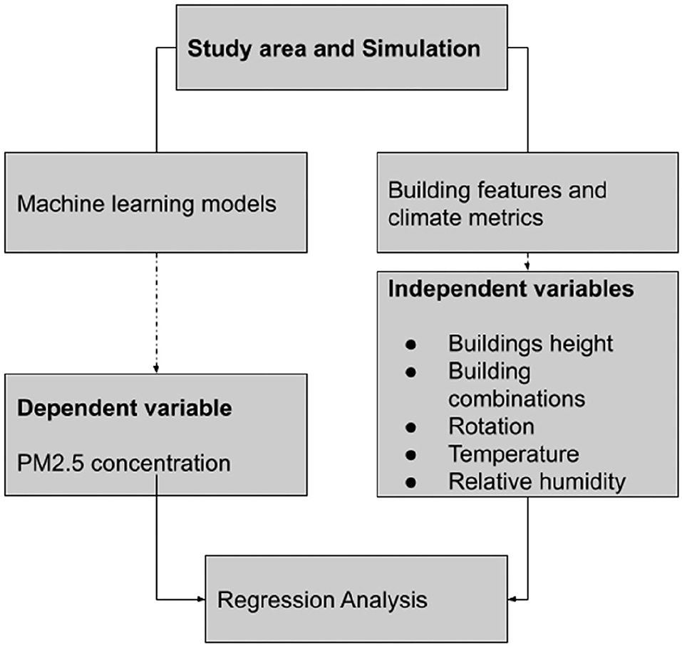
Figure 1. Research framework.

Method

Simulation scenarios

Four urban block typologies were examined: separated single blocks, separated L-shaped, C-shaped, and horizontal rows. The collected four-block typologies describe well-known typologies seen in the literature, and present cities (Figure 2). It is necessary to highlight that these examples depict common central areas and not the whole city typology. A study of more frequent typologies designates that single blocks are more prevalent in Asia (Seyedzadeh et al., 2018).

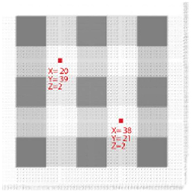
Figure 2. Schematic representation of the urban block fabric and urban block typologies.

In this research, simulation scenarios are divided into four groups. These divisions are based on the form that has several subsets in each group. There are constant materials in all scenarios; the tested variables in all groups change their general form, and in the subsets of each group, the height of the building and the quality of its different walls in terms of percentage of coverage with wall materials, including concrete walls, glass, and green walls. To examine the same conditions in different models and groups, it was necessary to select efficient points for all models. Furthermore, the changes in the discussed parameters can be checked after setting up the models and considering the climatic conditions of the two points selected for sampling. In the category of four groups, two points, A (X = 20, Y = 39, Z = 2) and B (X = 38, Y = 21, Z = 2), were analyzed, and the data was processed through ENVI-MET software, and Leonardo sub-program in the form of tables were extracted for each hour from the defined test interval. The cell resolution was set at 2 ^* 2 ^*2m (Figure 3).

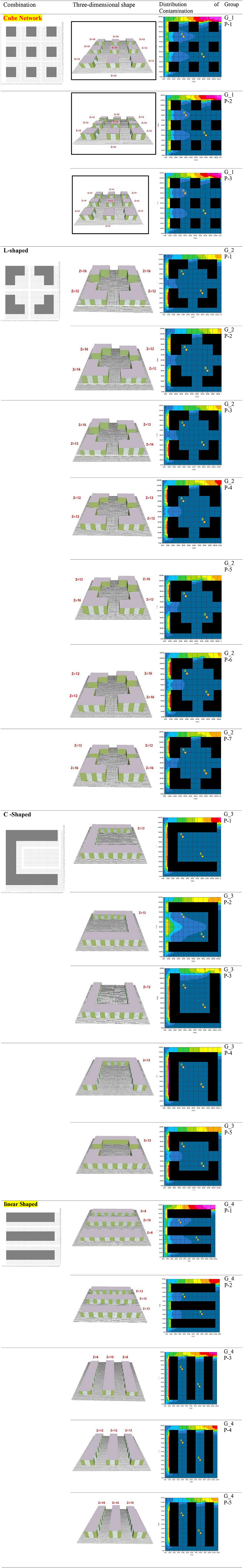
Figure 3. Selected sample point to compare.

The sheets extracted from the chart were tabulated in a table format and arranged in a row from 7 a.m. to 6 p.m., and in the columns, data such as wind flux on the axes, U, V, W, and wind speed were entered. In the defined direction, wind direction (which was fixed in our test and defined as 270°C), temperature, specific humidity, relative humidity, and information such as the number of different pollutants and the amount of sediment and its reaction were separated. These tables provide matrix data for using machine learning models. These parameters include temperature as one of the main factors in thermal comfort, relative humidity to study the effect of green walls and height changes on variations and moisture deposition, and the effect on thermal comfort and pollution concentration of 5.2 PM2, which was previously defined in the modeling stage. After preparing the data table, diagrams of temperature changes along with relative humidity and pollution concentration for each point were extracted in all patterns of all groups at 8 a.m. with the maximum pollution values.

In the last section, the machine learning models were applied data-driven from ENVI-MET software to find a prediction model. The design space in this research has five dimensions. The independent variables are temperature, relative humidity, height of the building, and pattern of combination buildings. The dependent variable is pollution concentration in two points, A and B.

The meaning of rotation in this research is the rotation of C-shaped, U-shaped, and linear patterns concerning the horizontal and vertical axes. Due to the change of direction of C and U and linear patterns, the rotation of the basic shapes is 90, 180, and 270°C on the horizontal and vertical axes.

Location and geographical conditions

The city of Tehran is located at 51° 24' 15.6348” E longitude and 35°42' 55.0728” N latitude. Its height above sea level ranges between 1,800 meters in the north to 1,200 meters in the center and 1,050 meters in the south.

Tehran is located between mountainous regions and plains. Three factors play an essential role in the climate in Tehran-the Alborz mountain range, humid westerly winds, and the province's size. In fact, in Tehran, the climate is temperate and mountainous, and in the lowlands, it is semi-arid. There is usually much rainfall in the winter. The cold season begins in December but a little earlier in the mountains and lasts for 3 to 4 months.

Materials

Several materials have been used in different sections which were available in the software database modeling the defined scenarios. The materials of all defined scenarios are the same. A list of materials with features and specifications is provided in Table 1.

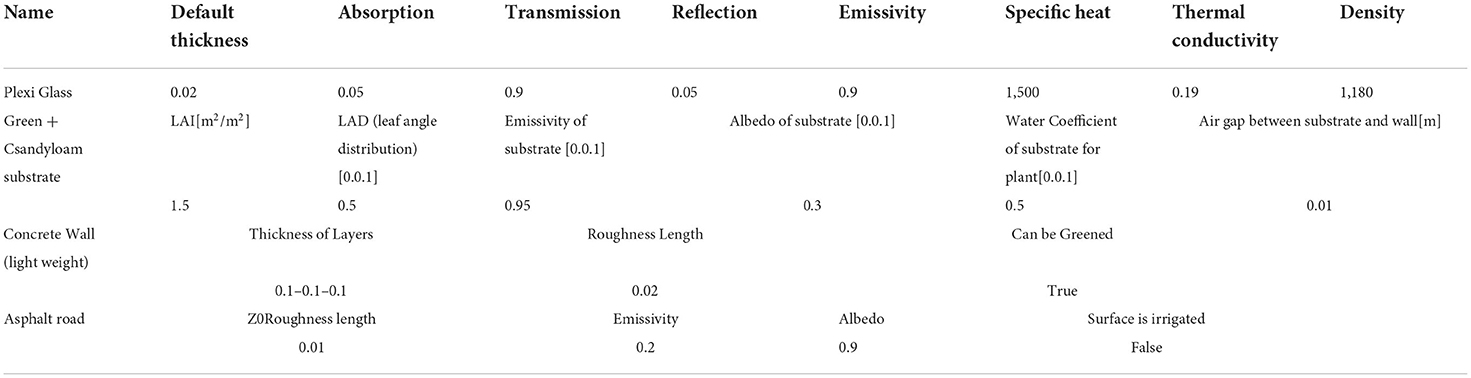
Table 1. Materials with features and specifications.

Sources of pollution

Modeling and placement of pollution sources and paths in each model were according to the scheme presented in Table 2. Since pollution concentration was significant for this research, the default sample was used in the software database, and the pollution profiles were not personalized.

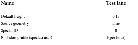
Table 2. Placement of pollution sources and paths.

Climate data

The climatic data specifications in this project are according to Table 3.

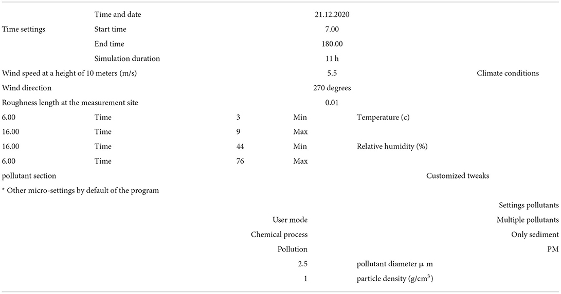
Table 3. Climate data.

Machine learning models

Machine learning models can evaluate input data characteristics based on model output results, saving time in computation and scenario simulation. Implementing the machine learning method involves a lot of time and accuracy due to the high number of parameters. Furthermore, the optimal composition of machine learning-based systems can efficiently manage the evolution of the variables, which is a worthy task for architects and designers—the possibility of development in model efficiency, utilization, and future directions (Seyedzadeh et al., 2018).

Regarding the hypothetical scope, this study applies a multimethod technique to examine the effect of building typologies on pollution concentration. Three statistical methods were used to examine the questionnaire responses: statistical technique, correlation examination, and regression examination. A polynomial regression model (PLR) identified the most influential factors throughout the sample's multiple-deviation data. The aspect prediction model was built based on the desegregated dataset from the simulation model. The model represents the Iranian context because the input data were drawn from simulations undertaken in Iran. However, the general methodology could be applied to other regions or countries. In the proposed model, PM2.5 in points A and B are used as input variables collected through data sampling and pre-processing. The subsequent paragraphs manifest the various methods applied in this study.

General framework

ML-based techniques have been used to predict the relationship between independent variables (temperature, relative humidity, and height of buildings among various groups) and the dependent variable PM2.5 in two different positions.

Polynomial regression model (PLR)

The polynomial regression model is a case of multiple regression with only one independent variable, X. This method involves two steps. First, a polynomial conversion of variables is undertaken, and second, multiple linear regression is applied.

Where k is the polynomial degree, which is the order of the model. Effectively, this method is the same as having multiple models. Coefficients and intercepts have a linear relationship that is predicted by these variables.

Multiple linear regression (MLR)

MLR aims to estimate the outputs by generating a linear equation between the explanatory (independent) variables and a response (dependent) variable (Makridakis et al., 2008):

Where x, y, and a present the independent, dependent, and random variables of the MLR typical formula sequentially, LR fits a linear model with coefficients b = (b1, …, bn) (2) to decrease the residual sum of squares between the perceived targets in the dataset and the targets predicted by the linear approximation. LR has been extensively studied and is widely used in the building science (Asadi et al., 2014).

Support vector regression

The system of support vector classification can be stretched to work regression obstacles. This method is called SVR. Moreover, the model provided by SVR depends only on a subset of the training data because the cost function neglects those examples where their forecast approaches their purpose. The investigation shows that strengthening the algorithms can also increase prediction accuracy. SVR operates on structural risk minimization based on the mathematical training hypothesis (Joachims, 1998) and it is superior to ANN in several criteria included in the training step. The computational time is also a significant element in regression assessment (Dhiman et al., 2019).

Equation (3) shows a linear regression function for forecasting, where x ϵ X is the input from all the attributes, w is the weight coefficient linked to every input vector x_i, and b is the bias expression.

Accuracy criteria

Two important accuracy scores should be considered when using ML techniques (Wei et al., 2019). The first is mean score error (MSE), which is the sum of the square residual (4), the goal of which is to minimize the MSE. The second is the R2 score (8). If the sum of the square residual is 0, then no errors exist, and the SS total is close to 1, which illustrates that the result is good (9). The optimization function finds m and c to minimize the MSE. The value of R2 is always between 0 and 1, that is, 0 ≤ R2 ≤ 1. An R2 value of 0.9 or above is outstanding, a value above 0.8 is good, and a value of 0.6 or above may be satisfactory in certain applications as described by the following formula (Ostertagová, 2012):

In all the preceding equations, Yi is real and μi is predicted.

Results and discussion

The relative humidity graph at point A is illustrated in Figure 4. In group one (a), the values and fluctuations are relatively proportional to the relative humidity and temperature in all three patterns. Maximum relative humidity decreased from 66 to 17% from 8 a.m. to 4 p.m. The relative humidity of 48% for all three groups at 4 p.m. was recorded as the minimum relative humidity. The difference in relative humidity in the three subgroups was 0.8% per hour and a maximum of 0.4%. The relative humidity decreased linearly from 8 a.m. to 4 p.m. and increased thereafter. At point A of group two (b), the relative humidity was similar to group 1. Its maximum value was reported at 8 a.m., and its minimum at 4 p.m. for each pattern. Pattern seven had the maximum value of 68.581% which was recorded at 8 a.m., followed by pattern three with 68.58%; the minimum was reported in pattern six with 48.92%. The maximum relative humidity difference in the patterns was 2% at 8 a.m. and 1% at 4 p.m. Hence the same behavior and values were recorded in all patterns. Unlike the previous two groups, in the relative humidity graph of group three at (c) in this group, the values do not follow a fixed pattern. At 8 a.m., when the highest relative humidity values were recorded for each pattern, the highest value was that of pattern two (68.979%).

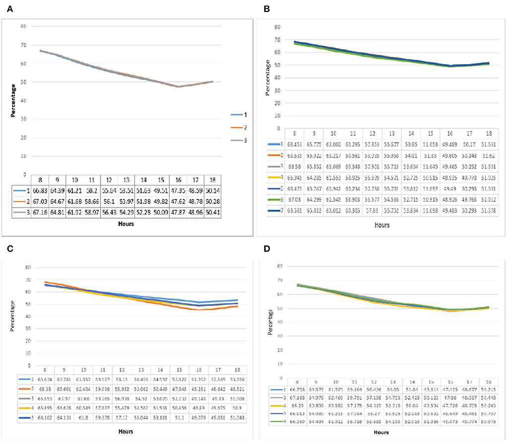
Figure 4. (A–D) Relative humidity comparison diagrams from point A in all groups, respectively.

In comparison, pattern two had the lowest level of relative humidity among the patterns at 4 p.m. (44.51%). The highest level of relative humidity fluctuations was recorded in pattern two with 24.4%, and the lowest level of fluctuations was recorded for pattern one with 12.3%. The graph of fluctuations in relative humidity in the fourth group (d) also showed similar behavior to the first three groups. The highest values for each pattern were recorded at 8 a.m. and then they had a decreasing trend until 4 p.m. and increased thereafter. The hourly variations for different patterns was below 2%. The highest value was reported at 8 a.m. for pattern one (67.758%), which also recorded the lowest at 4 p.m. (47.44%).

At point B in Figure 5, just as in point A of group one (e), a constant behavior and overlap of relative humidity and temperature graphs was noticeable in all three patterns. The maximum relative humidity for all three patterns was at 8 a.m., and the minimum was at 4 p.m. The difference between the relative humidity at the maximum hour was 0.3% and at the minimum hour was 0.8%. In the second group (f), the relative humidity graph showed a similar situation. With changes of about 1% between the patterns, it recorded relatively constant conditions in the defined period. The maximum relative humidity was at 8 a.m. and the minimum was at 4 p.m. The highest value was recorded for pattern one at 8 a.m. with 67.817% and the lowest value at 4 p.m. for pattern six with 51.009 %. The relative humidity graph for the third group (g) also followed the pattern of point A, and most fluctuations were seen in pattern two (24%). Some minor fluctuations were recorded in pattern one (13.6%). Also, the maximum relative humidity recorded at 8 a.m. for pattern two was 68.35%, and the lowest in group three was recorded for the same pattern at 4 p.m. (45.281%). The relative humidity diagram in the fourth group (h) follows the pattern and behavior of point A. The patterns at this point have the same variations with a difference of <1.5 percent in their values. The highest value was reported at 8 a.m. for pattern three (66.615%), and the lowest was recorded at 4 p.m. for pattern one (48.005 %).

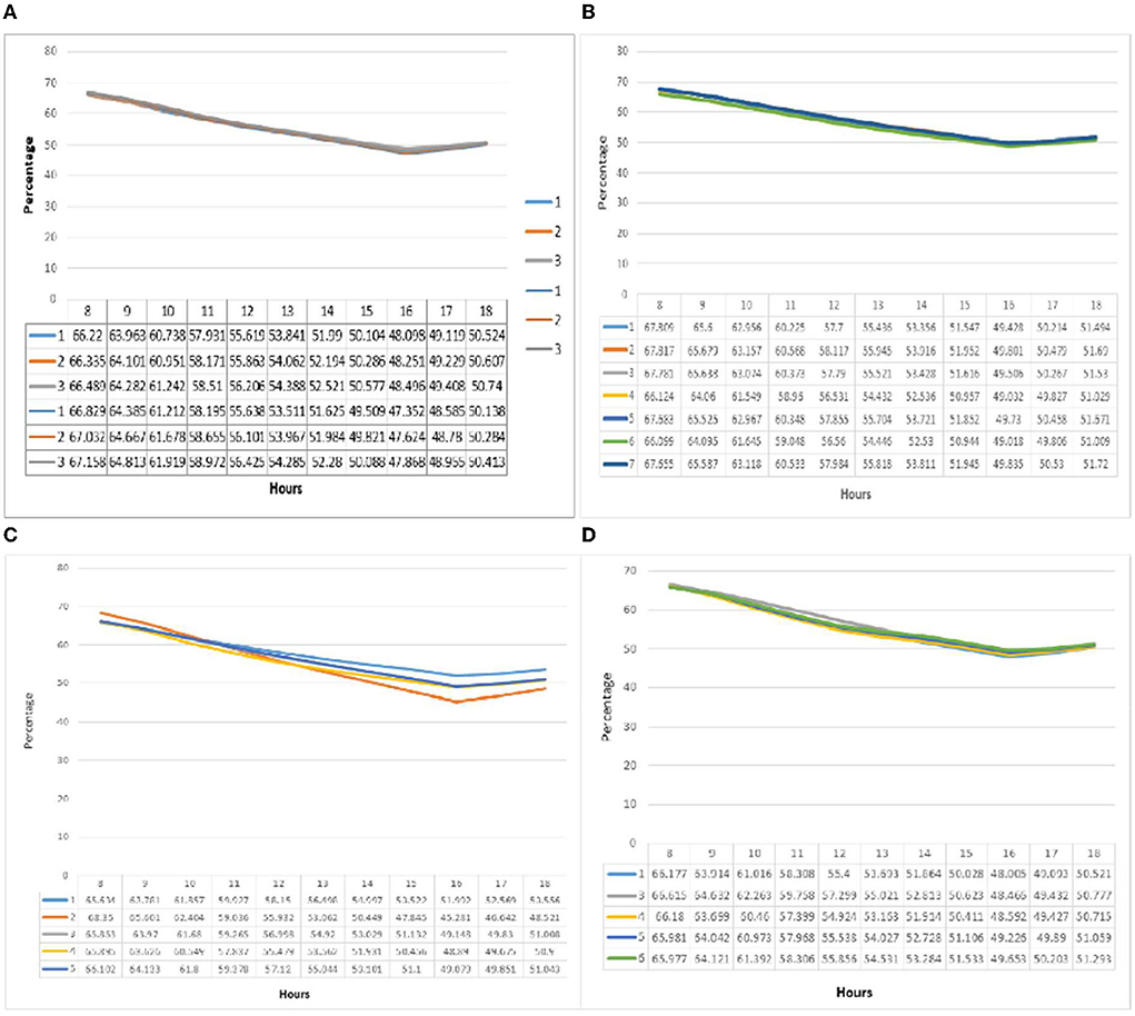
Figure 5. (A–D) Relative humidity comparison diagrams from point B in all groups, respectively.

It can be observed from the temperature graph in Figure 6 that group one (i) had almost the opposite behavior in relation to relative humidity. The minimum temperature at 8 a.m. was 5.3^°C, and the maximum at 4 p.m. was 8.4^°C. The temperature difference between the three subgroups was a minimum of 1.7% and a maximum of 1.3%. Following previous patterns, the minimum temperature in group two (j) was recorded at 8 a.m. and the maximum at 4 p.m. The highest value was related to patterns one and three, with a temperature of 8.14^°C at 4 p.m. The minimum temperature of 5.1^°C at 8 a.m. corresponded to pattern seven. The maximum temperature difference between the patterns at 4 p.m. was 10%, between patterns one and three (8.14^°C) and seven and five (7.39^°C). In patterns one and two, the temperature change diagrams in group three (k) behaved significantly different from the other three patterns. Patterns three, four, and five at 8 a.m. were in the range of 5^°C, and the hourly rate increased from 4 p.m. to 8.3^°C. Pattern one started from 17.68^°C, increased to 24.89^°C by 4 p.m., and decreased thereafter. Nevertheless, pattern two should have started with a slope greater than 9.58^°C and increased by 23.5^°C. Temperature changes in the fourth group (l) had an increasing slope until 4 p.m., the highest temperatures were recorded by patterns one and three at 4 p.m., and the lowest value was recorded at 8 a.m. in pattern five.

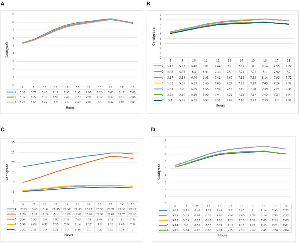
Figure 6. (A–D) Temperature diagrams from point A in all groups, respectively.

In the graph of temperature changes (Figure 7) in group one (m) at point B, similar to point A, the behavior of light is related to the relative humidity, which in all three patterns had an upward trend from 8 a.m. to 4 p.m. The slope was more than noon and decreased from 4 p.m. onwards. The maximum temperature difference between the three patterns was recorded at 1.2% at 8 a.m. and 1% at 4 p.m. In group two (n), temperature changes followed the previous samples to record the minimum at 8 a.m. and the maximum at 4 p.m. The highest temperature was recorded by pattern one with 8.13 ^°C at 4 p.m.; the lowest value was reported by patterns five and seven with 5.21 ^°C. The maximum difference during the test hours was less than one degree. Temperature changes in the third group (o) recorded behaviors similar to point A. The two patterns one and two, different from the other patterns, had an ascending behavior from 8 a.m. to 4 p.m.; the highest temperature recorded in pattern one was 24.72 ^°C. The slope of temperature increased, but similar to point A in pattern two, it was higher than in other patterns, from 9.76 ^°C at 8 a.m. to 23.09 ^°C at 4 p.m. The graph of air temperature changed in the fourth group (p) and was similar to previous patterns. Pattern six had a steeper slope than other patterns at 9 a.m. and was higher than at noon. Patterns four and five recorded lower values per hour than other patterns. The highest value was recorded at 4 p.m. for pattern six (8.17 ^°C).

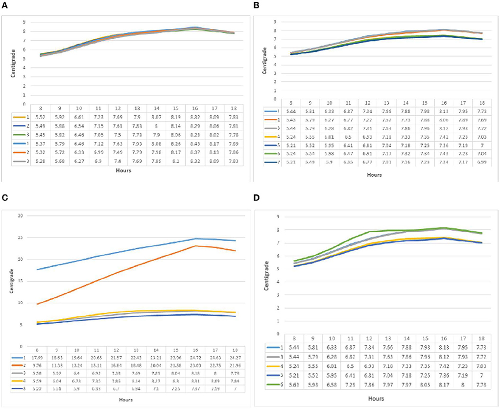
Figure 7. (A–D) Temperature diagrams from point B in all groups, respectively.

Figure 8 shows pollution concentration at point A. In the analysis of pollution concentration behavior in group one (a), what is shown in the modeling is relatively constant values from 8 a.m. to 11 a.m. in all three patterns, decreasing with a gentle slope from 11 a.m. onwards. The maximum amount of contamination for all three patterns was designated at 8 a.m. and the minimum at 6 p.m. Pattern one recorded the highest and the lowest amount of pollution per hour in the graph. So that the maximum value at 8 a.m. for pattern one was 0.241 micrograms per cubic meter and the minimum at 6 p.m. for the same pattern was 0.167 micrograms per cubic meter. The maximum difference between the three patterns at 8 a.m. was 40%, and the minimum difference at 6 p.m. was 33% between the three patterns. The maximum pollution concentration in group two (b) was at 8 a.m., which had a relatively stable trend until 10 a.m., after which it dropped downward. The highest value was recorded at 8 a.m. for pattern number six with a value of 0.094 μg / m3. The lowest value was reported at 6 p.m. as the pollution reduction hour for pattern two with a value of 0.060 μg / m3. The pollution concentration chart of group two patterns in point A can be deduced from the difference between patterns four and six and other patterns in the amount of pollution. At 8 a.m., the difference was about 10% higher on average than other patterns. Also, pattern two had a 10% decrease compared to other patterns and had the lowest value on the chart at point A of group two. In the third group (c), the concentration of pollution in pattern two in point A diagram recorded values up to four times compared to pattern five, which decreased after 10 a.m.

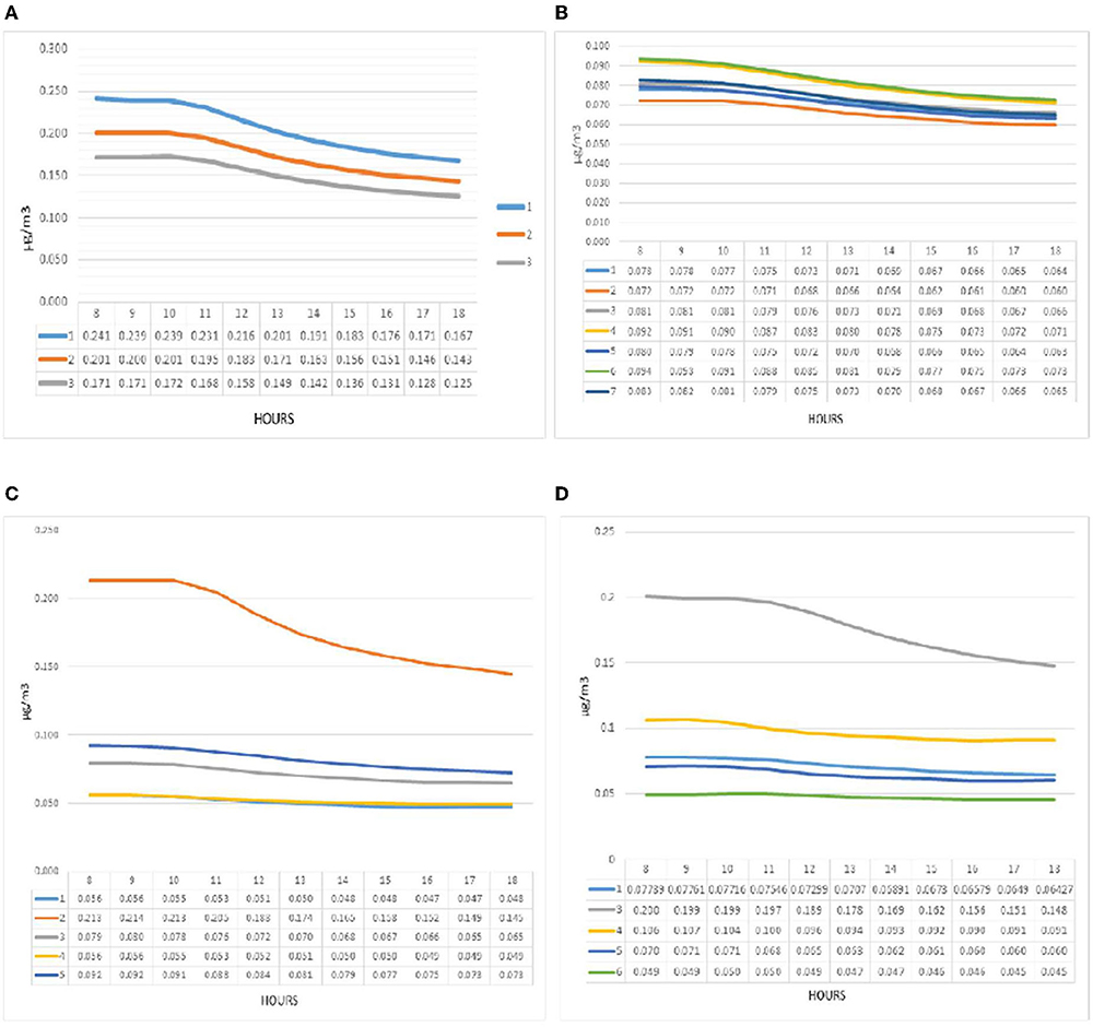
Figure 8. (A–D) Pollution concentration diagrams from point A in all groups, respectively.

In comparison, other patterns recorded significant differences and relatively constant changes. Patterns five and three at 8 a.m. showed values of 0.092 and 0.079 micrograms per cubic meter. The lowest values were recorded for patterns four and one with a difference of 0.056 and 0.054 μg. The highest concentration of pollution at this point was recorded in the fourth group (d) for pattern three, which was higher than other patterns, and recorded the highest value in this pattern by recording 0.2 micrograms per cubic meter at 8 a.m This pattern followed a decreasing trend since 11:16 a.m. with a uniform slope. These variations were much more minor for the other patterns, with the highest values recorded for patterns four, one, five, and six, respectively. The lowest value was set at 6 p.m. for pattern six (0.045 μg / m3).

Pollution concentration at point B is illustrated in Figure 8 in the first group (e), the amount of PM2.5 at point B has recorded a pattern similar to point A. The maximum amount of pollution was recorded at 8 a.m. and the minimum at 6 p.m. The highest (0.153) and the lowest (0.089) micrograms per cubic meter belonged to patterns 1 and 3, respectively, reported at 8 a.m. and 6 p.m. The pollution concentration chart in the second group (f) continued from 8 to 10 a.m. with a relatively zero slope and followed a decreasing trend. The highest pollution belonged to pattern four. At 8 a.m., it recorded 0.085 micrograms per cubic meter. The lowest values during the experiment at 4 p.m. were recorded by pattern two at 0.051 micrograms per cubic meter. In the third group (g), the concentration of pollution was shown at point B for some patterns different from point A, so pattern three was closer to patterns four and one. The maximum value in the maximum hour (8 a.m.) was 0.175 micrograms per cubic meter, which has decreased to 0.840 in pattern five and 0.048 in other patterns. The concentration of pollution in the fourth group (h) at point B for patterns one and three recorded significantly higher values than the other three patterns. Also, chart failure and pollution drop for these two patterns were more than in other patterns, while the other three recorded a linear and constant trend during the test hours. After patterns one and three, patterns four, five, and six had the highest pollution levels. The highest value at 8 a.m. was recorded in pattern one (0.192), and the lowest at 6 p.m. for pattern six (0.027).

Prediction models

An adequate data analysis contributes to an improved understanding of the results from ML algorithms and the objects being studied. Table 4 shows a detailed analytical description of twenty-six independent features and two dependent variables (PM2.5 in two points, A and B).

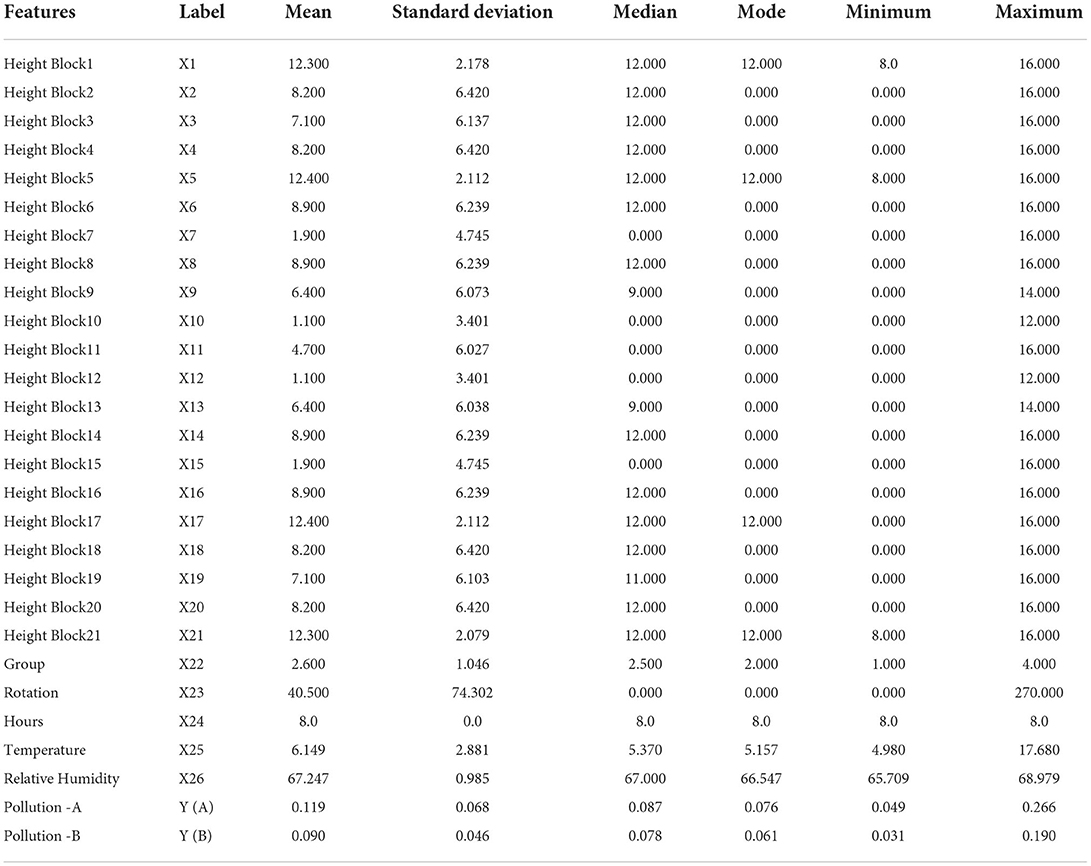
Table 4. Statistical analysis of features.

This study expected the ρ-value between independent variables to be in the range of 0 to 0.3 or −0.3 to 0, and the ρ-value between every independent variable with a dependent variable to be in the range of 0.7 to 1 or −1 to – 0.7. If this did not exist between variables, then the relationship between variables is nonlinear (Jacob et al., 2013). Table 5 and Figure 9 present the explanation of this correlation coefficient and position the relationship. In this study, the value of 0.40 between the group and rotation shows a good positive correlation between the variables, and −0.41 between the group and relative humidity demonstrates a good negative correlation. The p values obtained were <0.3, which indicates a lack of significance.

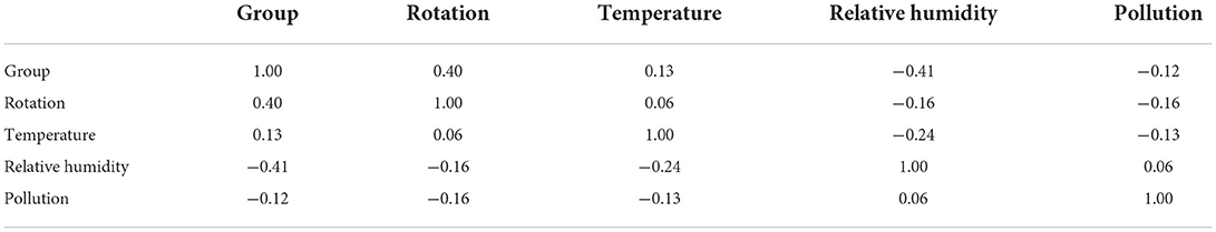
Table 5. Pearson's correlation coefficient among variables.

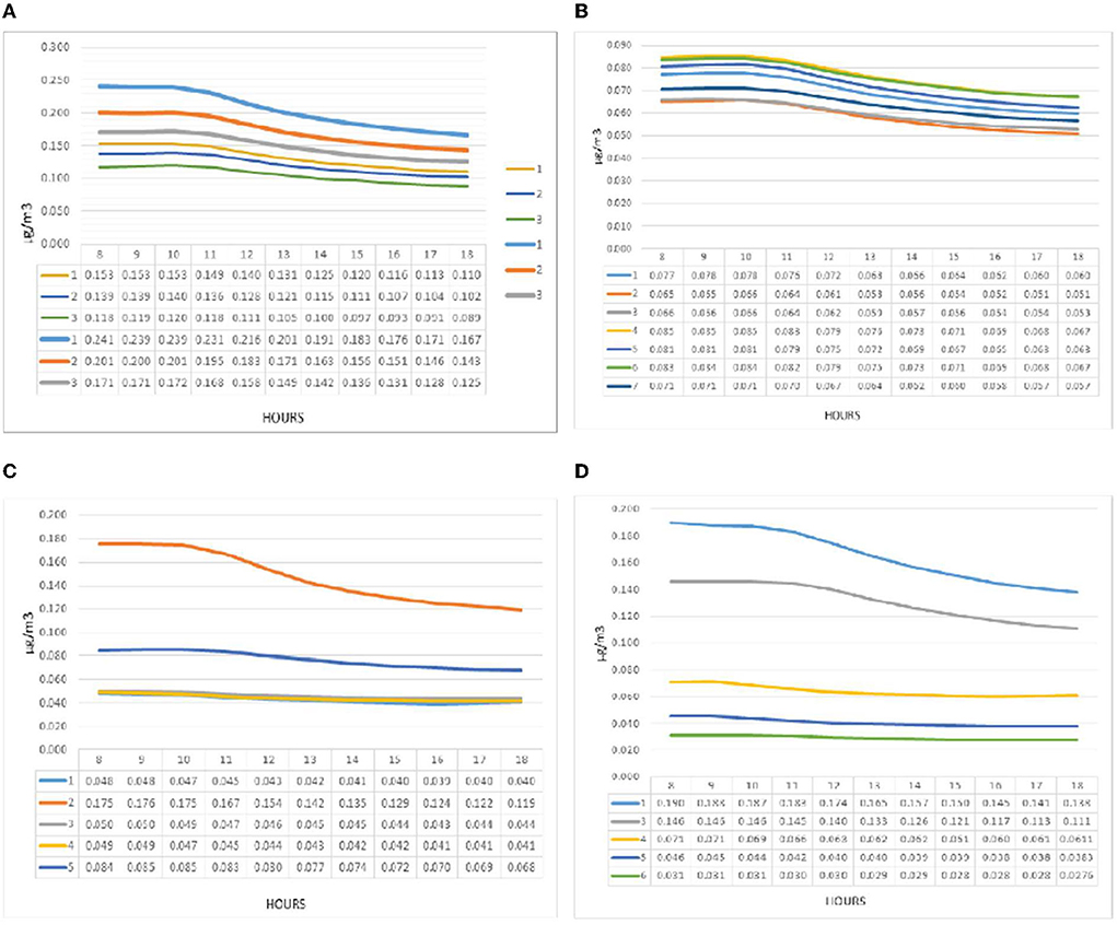
Figure 9. (A–D) Pollution concentration diagrams from point B in all groups, respectively.

The principal objective of this study was to investigate a prediction model for PM2.5 based on the various typology of buildings with the help of an ML approach. Table 6 shows that the model most capable of predicting the dependent variables from the independent variables was PLR. For predicting PM2.5 at points A and B, the PLR model yielded an R-square of 0.942 and 0.967, respectively, when the degree was three. The results are presented in Table 6. The PLR is an excellent model for measuring RME (4.648) and MAE (3.795) for point A and RME (2.552) and MAE (6.513). Furthermore, the high value of R2 for PLR (degree 3) presents a perfect adjustment between the real and measured PM2.5 for PLR approaches (Figure 10).

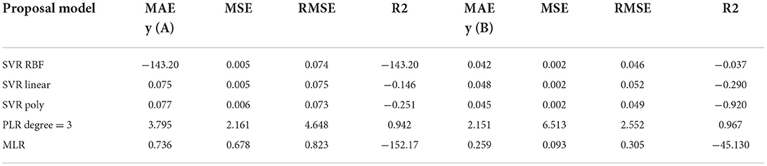
Table 6. Accuracy presentations of various models.

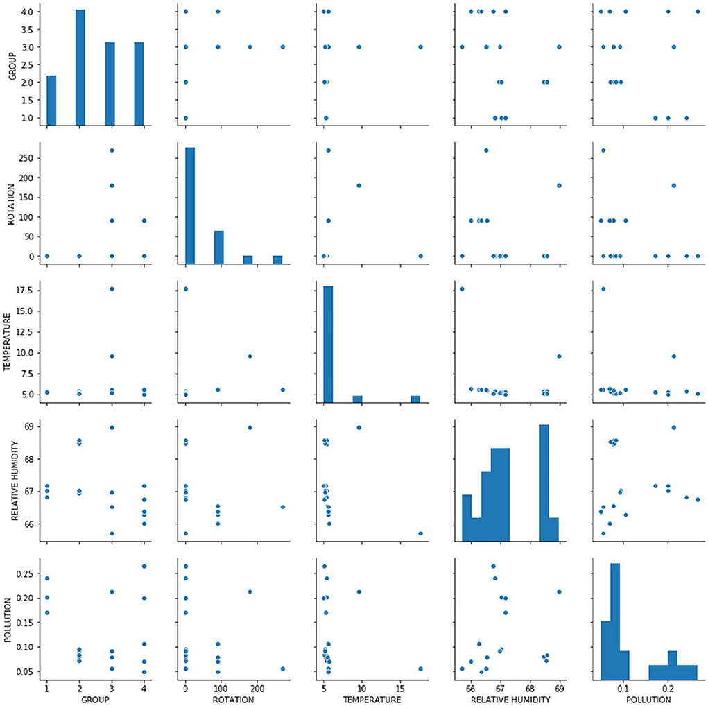
Figure 10. Pearson's correlation coefficient.

Conclusion

The performance of typologies in terms of temperature, relative humidity, and reduction of air permeability was strongly dependent on the blocks' orientation, the block shape's rotation concerning the horizontal and vertical extensions, the height of the blocks, and the type of typology. Accordingly, the performance was different in each of these studied typologies including cubic-shaped, L-shaped, C-shaped, linear-shaped, and courtyard.

Pollution concentration in the city depends on many elements, including block typology and environmental factors. This study aimed to find the prediction model between block typology and PM2.5.

In linear patterns, relative humidity behaved similarly for both east-west and north-south groups, and the lowest amount was at 4 p.m. The highest amount was at 8 a.m After 4 p.m., the relative humidity started to increase again. The air temperature was better for north-south linear patterns than east-west patterns. The thermal performance of such models was worst when all rows had a fixed height. When the middle row of blocks was taller, it performed better in terms of temperature.

The concentration of futures was the highest when the blocks are east-west, and the height of the blocks was constant. Moreover, the best collection performance in terms of reducing noise was related to the state where the direction of the rows was north-south, and the middle row was taller than the side rows.

In the central courtyard pattern, reducing the concentration of the front was optimal when the courtyard width was maximum. The air temperature worked better when the width of the yard was minimum. In other words, in these models, relative humidity performed better for samples with larger width yards.

In cubic models, air temperature and relative humidity changed almost identically at different hours of the day. The air temperature was the highest between 3 p.m. and 4 p.m. When the middle row was taller, the amount of distortion in these models was much more than in other cases.

In the L-shaped patterns, relative humidity had almost the same pattern. The emission concentration changed almost with a relatively constant slope for all samples. Nevertheless, there was a significant difference in the amount of pollution among the samples. The ensemble performance was much better when the windward front was taller. When the blocks were crosswise, the performance was optimal regarding the air temperature.

In the C-shaped patterns, the air temperature changed quite significantly. The pattern with a 2:1 central courtyard had a much more suitable function. Moreover, the pattern facing west was the worst performer in terms of measurable thermal comfort. Focusing on radiation was very unfavorable for C-shaped patterns when the opening of the C was toward the direction of the wind. When the opening was perpendicular to the direction of the wind, it had a very favorable performance in terms of reducing air pollution. The relative humidity changes in almost all samples follow a similar pattern. Air pollution was maximum between 8 a.m. and 10 a.m.

This study also developed a statistical ML framework to examine the effects of several independent variables on two dependent variables. The results showed that the PLR algorithm performed the best, suggesting that this particular algorithm can be used in other block typologies on pollution concentration.

Data availability statement

The raw data supporting the conclusions of this article will be made available by the authors, without undue reservation.

Author contributions

MK: paper draft, conceptualization, data collection, and valuation. MY: methodology, conceptualization, final editing, and literature. EP: literature and editing. All authors contributed to the article and approved the submitted version.

Conflict of interest

The authors declare that the research was conducted in the absence of any commercial or financial relationships that could be construed as a potential conflict of interest.

Publisher's note

All claims expressed in this article are solely those of the authors and do not necessarily represent those of their affiliated organizations, or those of the publisher, the editors and the reviewers. Any product that may be evaluated in this article, or claim that may be made by its manufacturer, is not guaranteed or endorsed by the publisher.

References

Allen, R. J., Turnock, S., Nabat, P., Neubauer, D., Lohmann, U., Olivi,é, D., et al. (2020). Climate and air quality impacts due to mitigation of non-methane near-term climate forcers. Atmos. Chem. Phys., 20, 9641–9663. doi: 10.5194/acp-20-9641-2020
Asadi, S., Amiri, S. S., and Mottahedi, M. (2014). On the development of multi-linear regression analysis to assess energy consumption in the early stages of building design. Energy Build. 85, 246–255. doi: 10.1016/j.enbuild.2014.07.096
Chang, C. C., Chen, P. S., and Yang, C. Y. (2015). Short-term effects of fine particulate air pollution on hospital admissions for cardiovascular diseases: a case-crossover study in a tropical city. J. Toxicol. Environ. Health A. 78, 267–277. doi: 10.1080/15287394.2014.960044
Chang, F. J., Chang, L. C., Kang, C. C., Wang, Y. S., and Huang, A. (2020). Explore spatio-temporal PM2.5 features in northern Taiwan using machine learning techniques. Sci Total Environ. 736, 139656. doi: 10.1016/j.scitotenv.2020.139656
Cihan, P., Ozel, H., and Ozcan, H. K. (2021). Modeling of atmospheric particulate matters via artificial intelligence methods. Environ. Monit. Assess. 193, 1–15. doi: 10.1007/s10661-021-09091-1
Daiber, A., Kuntic, M., Hahad, O., Delogu, L. G., Rohrbach, S., Di Lisa, F., et al. (2020). Effects of air pollution particles (ultrafine and fine particulate matter) on mitochondrial function and oxidative stress - implications for cardiovascular and neurodegenerative diseases. Arch Biochem Biophys. 696, 108662. doi: 10.1016/j.abb.2020.108662
Dhiman, H. S., Deb, D., and Guerrero, J. M. (2019). Hybrid machine intelligent SVR variants for wind forecasting and ramp events. Renew. Sust. Energ. Rev. 108, 369–379. doi: 10.1016/j.rser.2019.04.002
Ganesh, S. S., Arulmozhivarman, P., and Tatavarti, V. R. (2018). Prediction of PM 2.5 using an ensemble of artificial neural networks and regression models. J. Ambient. Intell. Humaniz Comput. 2018, 1–11. doi: 10.1007/s12652-018-0801-8
Jacob, C., Patricia, C., Stephen, G. W., and Leona, A. S. (2013). Applied Multiple Regression/Correlation Analysis for the Behavioral Sciences. Routledge. doi: 10.4324/9780203774441
Joachims, T. (1998). “Text categorization with support vector machines: Learning with many relevant features,” in European Conference on Machine Learning. Springer. doi: 10.1007/BFb0026683
Lelieveld, J., Evans, J. S., Fnais, M., Giannadaki, D., and Pozzer, A. (2015). The contribution of outdoor air pollution sources to premature mortality on a global scale. Nature. 525, 367–371. doi: 10.1038/nature15371
Li, X., Ma, Y., Wang, Y., Wei, W., Zhang, Y., Liu, N., et al. (2019). Vertical distribution of particulate matter and its relationship with planetary boundary layer structure in Shenyang, Northeast China. Aerosol Air Qual. Res. 19, 2464–2476. doi: 10.4209/aaqr.2019.06.0311
Liu, Q., Baumgartner, J., Benjamin de, F., and Schauer James, J. (2019a). A global perspective on national climate mitigation priorities in the context of air pollution and sustainable development. City Environ. Interact. 1, 100003. doi: 10.1016/j.cacint.2019.100003
Liu, Q., Wang, S., Zhang, W., Li, J., and Dong, G. (2019b). The effect of natural and anthropogenic factors on PM2.5: empirical evidence from Chinese cities with different income levels. Sci Total Environ. 653, 157–167. doi: 10.1016/j.scitotenv.2018.10.367
Liu, S., Xing, J., Zhao, B., Wang, J., Wang, S., Zhang, X., et al. (2019c). Understanding of aerosol–climate interactions in China: aerosol impacts on solar radiation, temperature, cloud, and precipitation and its changes under future climate and emission scenarios. Curr. Pollut. Reports. 5, 36–51. doi: 10.1007/s40726-019-00107-6
Makridakis, S., Wheelwright, S. C., and Hyndman, R. J. (2008). Forecasting Methods and Applications. New York, NY: John Wiley and Sons.
Motevalian, N., and Yeganeh, M. (2020). Visually meaningful sustainability in national monuments as an international heritage. Sustain. Cities Soc. 60, 102207. doi: 10.1016/j.scs.2020.102207
Norouzi, M., Yeganeh, M., and Yusaf, T. (2021). Landscape framework for the exploitation of renewable energy resources and potentials in urban scale (case study: Iran). Ren. Energy. 163, 300–319. doi: 10.1016/j.renene.2020.08.051
Obanya, H. E., Amaeze, N. H., Togunde, O., and Otitoloju, A. A. (2018). Air pollution monitoring around residential and transportation sector locations in lagos mainland. J. Health Pollut. 8, 180903. doi: 10.5696/2156-9614-8.19.180903
Ostertagová, E. (2012). Modelling using polynomial regression. Procedia Engineering 48, 500–506. doi: 10.1016/j.proeng.2012.09.545
Pu, Y., and Yang, C. (2014). Estimating urban roadside emissions with an atmospheric dispersion model based on in-field measurements. Environ Pollut. 192, 300–307. doi: 10.1016/j.envpol.2014.05.019
Sadaa, G. K. A., and Salihb, T. W. M. (2017). “Enhancing Indoor Air Quality for Residential Building in Iraq as a Typical Case of Hot Arid Regions,” in Proceedings of the Workshop on Indoor Air Quality in Hot Arid Climate, Kuwait. Kuwait City, Kuwait: Kuwait Institute for Scientific Research.
Sajani, Z. S., Marchesi, S., Trentini, A., Bacco, D., Zigola, C., Rovelli, S., et al. (2018). Vertical variation of PM2.5 mass and chemical composition, particle size distribution, NO2, and BTEX at a high rise building. Environ Pollut. 235, 339–349. doi: 10.1016/j.envpol.2017.12.090
Saleh, S., Rahimian, P., Farzad Glesk, I., and Marc, R. (2018). Machine learning for estimation of building energy consumption and performance: a review. Vis. Eng. 6, 1–20. doi: 10.1186/s40327-018-0064-7
Sovacool, B. K., Hook, A., Martiskainen, M., Brock, A., and Turnheim, B. (2020). The decarbonisation divide: contextualizing landscapes of low-carbon exploitation and toxicity in Africa. Global Environ. Change. 60, 102028. doi: 10.1016/j.gloenvcha.2019.102028
Sun, W., and Sun, J. (2017). Daily PM2. 5 concentration prediction based on principal component analysis and LSSVM optimized by cuckoo search algorithm. J. Environ. Manage. 188, 144–152. doi: 10.1016/j.jenvman.2016.12.011
Ventura, L. M. B., Pinto, F. O., Soares, L. M., Luna, A. S., and Gioda, A. (2019). Forecast of daily PM 2.5 concentrations applying artificial neural networks and Holt–Winters models. Air Quality, Atmosphere and Health 12, 317–325. doi: 10.1007/s11869-018-00660-x
Wang, H., Wang, Q., Gao, Y., Zhou, M., Jing, S., Qiao, L., et al. (2020). Estimation of secondary organic aerosol formation during a photochemical smog episode in Shanghai, China. J. Geophys. Res. Atmos. 125, e2019JD. doi: 10.1029/2019JD032033
Wang, Z., and Liu, J. (2018). Spring-time PM2, 5. elemental analysis and polycyclic aromatic hydrocarbons measurement in High-rise residential buildings in Chongqing and Xian, China. Energy Build. 173, 623–633. doi: 10.1016/j.enbuild.2018.06.003
Wei, G., Jalal, A., Hossein, M., Amin, S., and Hong, N. (2019). Comprehensive preference learning and feature validity for designing energy-efficient residential buildings using machine learning paradigms. Applied Soft Comput. 84, 105748. doi: 10.1016/j.asoc.2019.105748
Xue, T., Zheng, Y., Tong, D., Zheng, B., Li, X., Zhu, T., et al. (2019). Spatiotemporal continuous estimates of PM2.5 concentrations in China, 2000-2016: a machine learning method with inputs from satellites, chemical transport model, and ground observations. Environ Int. 123, 345–357. doi: 10.1016/j.envint.2018.11.075
Yanlai, Z., Fi-John, C., Li-Chiu, C., I-Feng, K., Yi-Shin, W., and Che-Chia, Y. (2019). Multi-output support vector machine for regional multi-step-ahead PM2. 5 forecasting. Sci. Total Environ. 651, 230–240. doi: 10.1016/j.scitotenv.2018.09.111
Yeganeh, M. (2020). Conceptual and theoretical model of integrity between buildings and city. Sustain. Cities Soc. 59. doi: 10.1016/j.scs.2020.102205
Yeganeh, M., Bayegi, F., and Sargazi, A. (2018). Evaluation of environmental quality components on satisfaction, delight and behavior intentions of customers (case study: Gorgan restaurants). Am. J. Res. 5–6. doi: 10.26739/2573-5616-2018-3-2-10
Keywords: block typology, pollution concentration, regression models, machine learning, building
Citation: Karimian Shamsabadi M, Yeganeh M and Pourmahabadian E (2022) Urban buildings configuration and pollutant dispersion of PM 2.5 particulate to enhance air quality. Front. Sustain. Food Syst. 6:898549. doi: 10.3389/fsufs.2022.898549
Received: 17 March 2022; Accepted: 26 July 2022;
Published: 26 September 2022.
Edited by:
Riccardo Buccolieri, University of Salento, ItalyReviewed by:
Adriano Magliocco, University of Genoa, ItalySaiful Irwan Zubairi, National University of Malaysia, Malaysia
Copyright © 2022 Karimian Shamsabadi, Yeganeh and Pourmahabadian. This is an open-access article distributed under the terms of the Creative Commons Attribution License (CC BY). The use, distribution or reproduction in other forums is permitted, provided the original author(s) and the copyright owner(s) are credited and that the original publication in this journal is cited, in accordance with accepted academic practice. No use, distribution or reproduction is permitted which does not comply with these terms.
*Correspondence: Mansour Yeganeh, yeganeh@modares.ac.ir