Building “First Expire, First Out” models to predict food losses at retail due to cold chain disruption in the last mile

Introduction

Supply chain management of temperature sensitive products such as perishable food commodities throughout the cold chain is very challenging. Cold chain, a version of supply chain, focuses on maintaining product integrity and quality through temperature management from product origin to the final consumer (Global Cold Chain Alliance, 2020). A “break” in cold chain leads to temperature abuse (TA; Ndraha et al., 2018) which can occur during transportation and ultimately affects food safety and shelf-life of the products. TA during the last mile of the cold chain can push the foods into the “danger zone” defined as temperature between 40 and 140°F or 4 and 60°C which creates an environment conducive for the growth of spoilage and pathogenic microorganisms (Labuza and Fu, 1995; Oscar, 2009; United States Department of Agriculture, 2021). Hence foods are kept out of the “danger zone” temperatures to mitigate food safety risks (Godwin et al., 2012). Moreover, TA during supply chain can lead to faster food spoilage contributing to the global food loss (before retail) and waste (retail and beyond) problems causing economic losses and food security issues. In the U.S. alone, food waste is as high as 40%, and 133 billion pounds may be lost at the levels of retail and consumption (United States Department of Agriculture, 2022a). Addressing the food waste problem is important to feed a continuously growing population which could reach 8.5 billion by 2030 (United Nations, 2022a) of which an estimated 660 million may be battling hunger (United Nations, 2022b). Hence, it is important to study the effects of TA during transportation, its impact on the spoilage of foods and develop practical methods to predict shelf-life to reduce food waste and loss.

Transportation of foods from the processor or distributor to the retailer or final consumer is primarily done using two popular shipping methods: (1) Full Truckload (FTL) and (2) Less-Than-Truckload (LTL; Vega et al., 2021). In contrast to FTL, LTL shipping is utilized when the cargo requires only a portion of the space in a trailer (FedEx, 2022) such that the shipper does not pay the rent of an entire truck but only for the space their cargo occupies (Özkaya et al., 2010). One of the biggest challenges of LTL is understanding the “last mile” problem (Deutsch and Golany, 2018). The last mile is the last segment of a supply chain where product is transported to the end user (Shu et al., 2015). During the last mile, temperature fluctuations and condensation can occur on perishable food products (Mirzaee and Bishop, 2009) potentially due to the LTL delivery vehicle making multiple stops during the last mile (Aljohani and Thompson, 2020). Addressing how to best approach last mile problems is a key component of the United States Food and Drug Administration (2021) (FDA) “New Era of Smarter Food Safety” and can help regulatory bodies to further strengthen the food supply chain. Skawińska and Zalewski (2022) proposed the use of real time temperature monitoring using various technologies as an effective tool in the food cold chain. Additionally, research has been conducted to improve the design of reefer trucks and introduce new components to the container itself to improve air circulation, establish loading/unloading patterns, and improve cooling efficiencies (Tassou et al., 2009; Rai et al., 2019; So et al., 2021). Also, de Frias et al. (2020) investigated the temperature implications of opening doors to a refrigerated display case with the most extreme scenarios (opening every 5 min for 60 s) resulting in significant differences in product temperature. Additionally, they found that TA can occur with temperatures as high as 6.6°C when the doors are opened in regular intervals and durations. Much research has been conducted on the effects of TA on the safety (Wen and Dickson, 2012; Chen and Meng, 2021) and spoilage (Reddy et al., 1995; Rogers et al., 2014) of various food products. However, there is a gap in the literature on the effects of LTL TA during the last mile at the pallet level for temperature sensitive products. This is an important gap to fill as it mimics the real-world scenario providing a more pragmatic insight into the problem compared to studies conducted on individual pieces of food in controlled laboratory settings.

Another implication of TA during LTL can be on product rotation decision making at the retail level. The traditional product rotation model of “First In, First Out” (FIFO) operates under the assumption that products that arrive first should be rotated out first because they will expire first (Pikora et al., 2021). In contrast, the “First Expire, First Out” (FEFO) model takes into consideration the remaining life of a product (Mendes et al., 2020) which can be impacted by the temperature of the refrigerated trailer. The temperature inside refrigerated trailers are not homogeneous therefore, the level of TA experienced by products placed at different locations inside a refrigerated truck may be different (Jedermann et al., 2009; Getahun et al., 2017). do Nascimento Nunes et al. (2014) demonstrated the heterogeneity of temperature of a pallet of berries and demonstrated the FIFO model leads to the waste of high value temperature sensitive products. The FEFO model has been suggested to be a superior to FIFO in food (Curto and Gaspar, 2021) as well as non-food products, such as pharmaceuticals (Sukasih et al., 2020; Rezeki et al., 2022). One of the primary challenges of FEFO is it requires information sharing between different members of the cold chain (Hertog et al., 2014). However, in vertically integrated industries, such as poultry (Vukina, 2001), information sharing is much easier. Also, the development of technologies (e.g., RFID) has made the use of a dynamic shelf-life more realistic (Grunow and Piramuthu, 2013; Gaukler et al., 2017). Through our research, we have further emphasized the significance of the FEFO model and provided mathematical equations to predict shelf-life that can reduce food waste at the retail level.

Building mathematical models requires significant amount of data collected repeatedly over a period of time which is a daunting and an expensive task so researchers often use simulation models. Simulation models (e.g., Monte Carlo) can be powerful tools that enable the user to play the “what if?” game and perform risk analysis. Monte Carlo methods (MC) have been used in a wide variety of fields due their wide range of applicability (Raychaudhuri, 2008). In agriculture MC have been used to estimate proportions of crops in Kenya (Maeda et al., 2010), estimate the feasibility of alternative farming methods in Tanzania (Kadigi et al., 2020), and estimate the risks associated with pesticide use in Iran (Eslami et al., 2021). Even when narrowing the scope to a single industry (e.g., the poultry industry) MC methods have been investigated extensively. Rico-Contreras et al. (2017) used MC to estimate economic risk associated with different moisture levels of poultry litter used for energy production. A study using MC was done in the United Kingdom to determine the environmental impact of the 4 major types of egg production systems (Leinonen et al., 2012). MC were used to investigate the impact of predetermined parameters on the likelihood of Salmonella infection from the consumption of a common chicken dish in South Korea (Jeong et al., 2018). MC have been previously used by researchers to estimate the remaining shelf-life of both food and pharmaceutical products (Waterman et al., 2007; Lau et al., 2022). In an experiment on milk, shelf-life was investigated with MC being used to construct probability distributions of storage temperature, initial bacterial concentration, and generation times (Schaffner et al., 2003). Giannakourou and Taoukis (2019) utilized MC with cold chain distribution and temperature data. They were able to compare the shelf-life predictions of their model with shelf-life predicted by the “use-by” date, and they concluded that the uncertainty calculations built into their model resulted in more accurate shelf-life predictions. Additionally, Giannakourou et al. (2001) investigate the applicability of a shelf-life decision system (SLDS). They implemented MC to simulate the results of the SLDS method, and they determined in local markets 12% and 2% of products were spoiled at the time of consumption for the FIFO system and the SLDS system, respectively. Because of its previous use in similar applications, we believe MC could be applied to the LTL TA problem discussed. The objectives of this study are to investigate the effects of LTL TA during the last mile at the pallet level on the shelf-life of temperature sensitive products and to provide a potential solution through predictive models using MC.

Materials and methods

Experimental design

A commercially produced 1,000 lb pallet of boneless, skinless chicken breast filets (4 layers/pallet x 5 boxes/layer x 24 trays/box x 3–6 filets per tray) from a USDA inspected processing facility was procured and used to measure the temperature of filets (n = 20) in boxes during simulated 24 h of simulated LTL TA (2 h at 4°C, then 2 h at 25°C) for 5 independent trials. Next, microbial sampling was conducted (3 filets/box x 2 preselected boxes/layer) before TA (0 h) and immediately after TA (24 h). Additional microbial sampling was conducted (3 filets/box x 2 preselected boxes/layer) on alternating days (2, 4, 6, 8) after the LTL TA portion of the experiment to determine the rate of spoilage for all 5 trials. Lastly, using temperature and microbial data from the 5 trials, two separate MC methods were developed. Figure 1 outlines the methodology followed during this research.

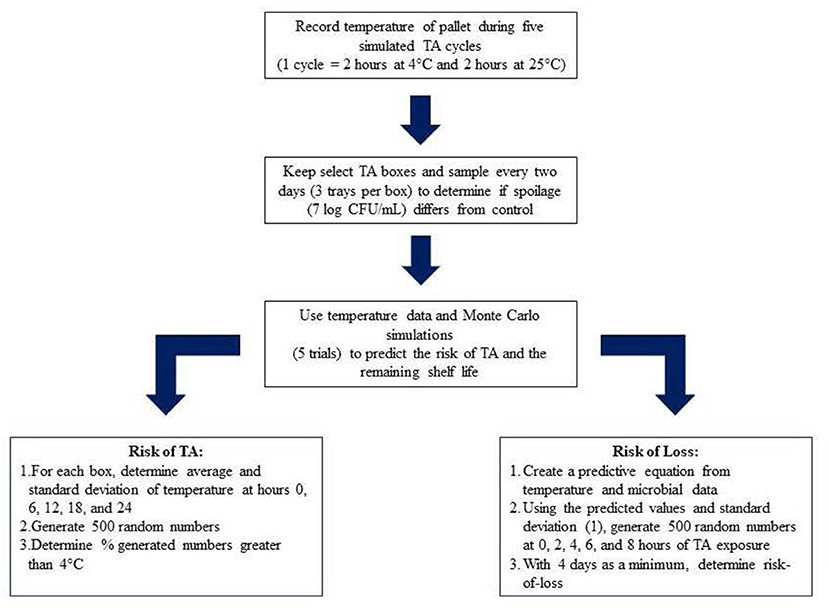
Figure 1. Flow diagram of research methodology for the development predictive models of less-than-truckload temperature abuse.

Recording filet temperatures

Raw chicken breast filets were used as a model for the study as it is the most affordable and popular protein source (National Chicken Council, 2022a,b) but at the same time it is also a highly perishable food with low temperature storage (4°C) being the common way to preserve it.

Raw chicken breast filets packed in trays, placed in boxes which in turn were stacked on a pallet were transported to the Charles C. Miller Jr. Poultry Research Center at Auburn University under refrigeration and stored in a walk-in cooler (4°C for 12–16 h) prior to experimentation. The boxes were serially marked from 1 to 20 (layer 1: 1–5; layer 2: 6–10; layer 3: 11–15 and, layer 4: 16–20). The boxes comprising the pallet had industry standard holes on the sides for moving, and the pallet was wrapped in plastic wrap to provide stability. Temperature at the center of a single representative breast filet in each box was continuously measured every 1 min for 24 h using TM500 12-channel thermocouple dataloggers with wire temperature probes (Extech Instruments, Nashua, New Hampshire, USA). The tray located approximately in the center of each box was chosen. Next, the thermocouple wire was inserted through the plastic film and into the center of the middle filet in the tray, and the wire was secured via sous vide tape. In each box, a second thermocouple wire was left loose to record air temperature resulting in two wires per box. At the conclusion of the experiment, temperature data was retrieved from the data loggers using MS Excel (Version 16, Microsoft Corporation, Redmond, WA). This experiment was repeated 5 separate times, and the temperature patterns were analyzed using line graphs generated using MS Excel.

Simulated temperature abuse

TA during LTL was simulated as follows: the pallet was exposed to 2 h at 4°C, simulating a refrigerated truck, and 2 h at 23 ± 2°C, simulate hypothetical TA that occurs when the truck doors are opened and closed. The experiments were conducted by moving the pallet in and out of a walk-in cooler maintained at 4°C for a total of 6 TA cycles (1 cycle = 2 h at 4°C, then 2 h at 25°C). A separate representative box was kept in the walk-in cooler for the duration of the 24 h experiment which acted as the control. The temperature of the control box and the outside room temperature were recorded with a probe thermometer every 2 h.

Thermal imaging

During the TA trials, thermal images of the pallet were taken using an infrared camera (BCAM 9 Hz 120 x 120 Thermal Infrared Camera, Teledyne FLIR, Wilsonville, OR, United States) every 2 h of the experiment. The camera was pointed centrally at the pallet from all four sides at a distance of 4 ft when shooting images. Thermal images were always taken when the pallet was in the outside room (either immediately after being removed from the walk-in cooler or immediately before). The images were saved to a removable memory card in the camera and were retrieved at the conclusion of each trial of the experiment.

Spoilage study

Microbiological sampling was conducted before (0 h) and immediately after the end of the simulated TA (24 h) to determine if TA immediately impacted the bacterial levels of the raw poultry breast meat. Two predetermined boxes were chosen from each layer to have microbial sampling. The boxes sampled were as follows: layer one: boxes 1 and 4, layer 2: boxes 7 and 10, layer 3: boxes 12 and 14, and layer 4: boxes 17 and 19. These boxes were selected based on their position within each layer (1 perimeter box and the center box). Two tray packs were randomly chosen from each box and 1 filet per tray was sampled for microbiological analysis. One filet from each selected tray pack was aseptically placed in a sterile bag (18 x 30 cm, 1,650 ml, VWR, Radnor, PA, United States) and manually rinsed with 50 ml of sterile buffered peptone water (Neogen Corporation, Lansing, MI) for 1 min, and the rinsate was serial diluted and spread plated in duplicate onto Standard Methods Agar Petri plates (Neogen Corporation). The Petri plates were incubated either at 37°C for 24–48 h to estimate aerobic plate counts (APC) or at 4°C for 10 days to estimate psychrotrophic plate counts (PSY). After the incubation period, viable colonies on the Petri plates were counted and reported as log CFU/ml of rinsate.

Shelf-life assessment of raw breast filets after temperature abuse

The effect of TA on the changes in shelf-life of raw chicken breast meat was assessed using 2 boxes from the TA abused pallet. The trays from the 2 boxes that crossed 4°C the fastest were pooled together, stored at 4°C, and sampled for microbiological analysis every 2 days until the APC counts reached 7 logs. Control chicken trays were stored and sampled in a similar manner. During each sampling time, 3 trays from the TA and control samples were sampled in the same manner as in the spoilage study. Plates were counted after 24 h (APC) and 10 days (PSY) and a two-sample equal variance t-test was performed using Excel at each sampling day to determine if bacterial concentrations are significantly different at the chosen sampling times.

Monte Carlo simulations

Two methods were developed using MC simulations. One method predicts the risk of TA based on box number, and the other predicts the remaining shelf-life according to the level of TA experienced. The simulations allow us to take our existing data at specific time points and increase it to a large degree. The data generated through these simulations enabled us to develop predictions based on 500 data points rather than only using the limited amount of data acquired through physical testing. For the first method, MC simulations using temperature data from h 0, 6, 12, 18, and 24 were performed. Temperature recordings from 4 or 5 of the trials at these time points was used to calculate an average temperature and standard deviation of temperature for each box at each time point. Next, using the mean and standard deviation, we generated a random number using the Excel formula: NORMINV(rand(),mu,sigma). In this formula, rand() creates a random value between 0 and 1, mu is the sample mean, and sigma is the sample standard deviation (Winston, 2022). When using this formula, the user is calculating the pth percentile of a normal random variable occurring with the chosen mean and standard deviation (Winston, 2022). Following the initial number generation, 500 iterations were run at each timepoint for each box. From the 500 generated numbers, we obtained an average, standard deviation, maximum, and minimum temperature for each box at each time point. Lastly, we calculated what percentage of the 500 numbers was >4°C at each time point. Formula 1 illustrates how risk of TA was calculated with n_>4 being the number of simulations >4°C.

The second method used temperature data and APC data from the control and TA filets. The remaining shelf-life was calculated for 3 control filets (0 h >4°C) and 3 TA filets (8 h >4°C). A graph was constructed with shelf-life graphed vs. time >4°C. Next, a trendline was fit to the data and a linear regression equation was obtained (Formula 2).

Estimates of shelf-life were obtained for different levels of TA by substituting values in for “x” (0, 2, 4, 6, and 8 h) and solving for “y.” The shelf-life values (y) and a standard deviation (1) were used to run MC simulations (500 iterations) in the same manner as previously described using Excel. From the 500 generated numbers, the percentage <4 days was calculated. This value is referred to as “risk-of-loss” because of the assumption retailers cannot sale all the product before spoilage in under 4 days. Formula 3 shows how risk-of-loss was calculated with n_<4days being the number of simulations that resulted in <4 days of shelf-life.

Results and discussion

Temperature profile

Temperature profiles of all the four layers of the pallet show peaks and valleys reflecting TA and were more pronounced in the top and bottom layers (Figures 2, 5) than in the middle layers (Figures 3, 4). All the boxes in layer 1 crossed 4°C by ~12 h (Figure 2) likely because the top layer of the pallet is more exposed than the other layers with the sides being in contact with the air surrounding the pallet. Temperature profile of the top layer indicates that product in this layer is most prone to rapid spoilage and should be treated the most differently. Similarly, layer 4 had all but one box (box 19) cross 4°C by 24 h (Figure 5) as the layer is in direct contact with the wooden pallet which is in direct contact with the floor resulting in more dramatic influence by the TA. The middle 2 layers of the pallet (Figures 3, 4) were less impacted as shown by the less dramatic increase in temperature. In the middle layers, most of the boxes never reached 4°C with only boxes 6 and 13 crossing 4°C for layers 2 and 3, respectively. In layers 2 and 3 of the pallet (Figures 3, 4) boxes are shielded by the top and bottom layers. Also, the pallet has a plastic wrap (a standard industry practice) applied around the perimeter of the box which may be helping the middle 2 layers stay insulated and less impacted by the TA. The deviation from the target temperature (4°C) seen in our simulated supply chain resemble those recorded from an actual supply chain in South Africa (Emenike and Hoffman, 2014). Similar to our study, Emenike and Hoffman (2014) used dataloggers, however their target temperature was 2°C, and the data loggers were placed along the periphery of a reefer truck and not in individual boxes on a pallet. Emenike and Hoffman (2014) reported average transportation temperatures as high as 14.9°C which could be due to the inadequate cold chain in South Africa compared to other countries with more developed cold chains. A similar mismatch of the target cold chain temperature was reported by Ndraha et al. (2019) who studied the temperatures of frozen shrimp in the last mile before home deliveries. While the shrimp were not being shipped on pallets at this stage, the temperature results had similar findings to ours in that the target temperature (−18°C) was often not the temperature of the products being shipped. In fact, they found the shrimp were above the target temperature over 50% of the time.

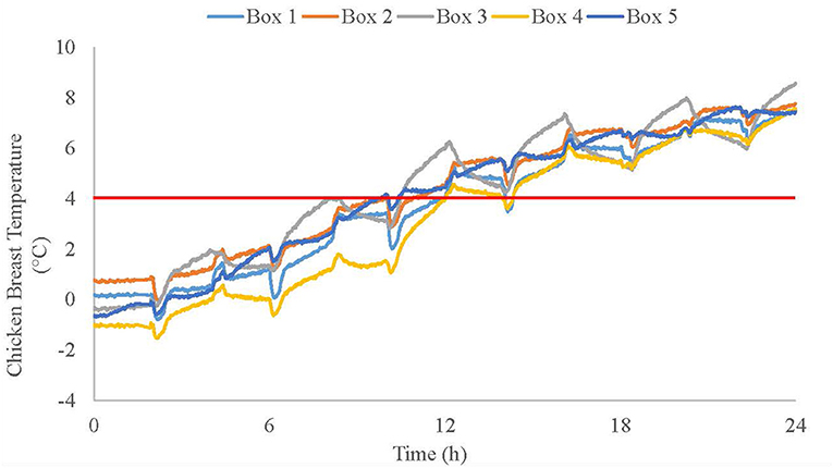
Figure 2. Averaged temperature profiles (4 replications) of top layer (layer 1) boxes of palletized chicken breasts while experiencing simulated LTL cyclic TA (2 h at 4°C then 2 h at 25°C).

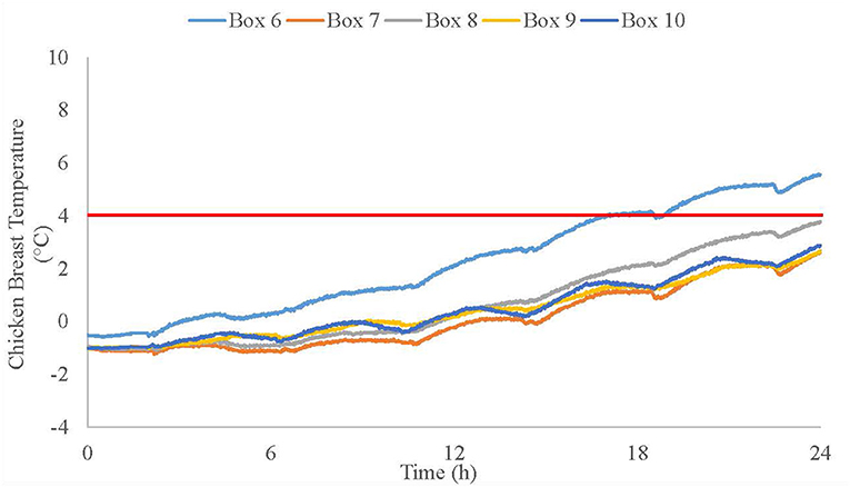
Figure 3. Averaged temperature profiles (4 replications) of second layer from the top (layer 2) boxes of palletized chicken breasts while experiencing simulated LTL cyclic TA (2 h at 4°C then 2 h at 25°C).

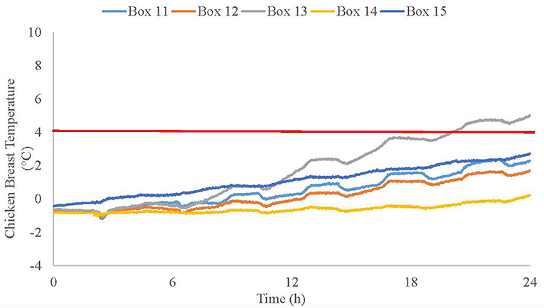
Figure 4. Averaged temperature profiles (4 replications) of third layer from the top (layer 3) boxes of palletized chicken breasts while experiencing simulated LTL cyclic TA (2 h at 4°C then 2 h at 25°C).

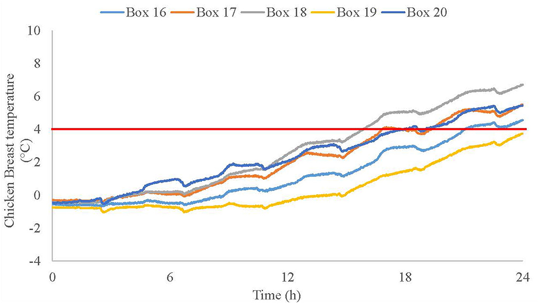
Figure 5. Averaged temperature profiles (4 replications) of bottom layer (layer 4) boxes of palletized chicken breasts while experiencing simulated LTL cyclic TA (2 h at 4°C then 2 h at 25°C).

Figure 6 shows a schematic of how the boxes are arranged on the pallet. Figure 6 was rendered from the temperature graphs for a rapid analysis of the boxes which crossed 4°C and the corresponding time (h). The boxes are color coded for each layer according to the order in which they reached 4°C. Regarding the severity of TA, the box order is as follows from hottest to coldest: red, orange, yellow, blue, and purple. The impact of box position is indicated by the colors in each layer. In all layers, the centrally placed box is colored purple indicating it was either the least abused box or it never crossed 4°C (Figure 6). Also, the most abused box was always a perimeter box. In the case of layers 2, 3, and 4, the most TA box were stacked at the same location of the pallet (Figure 6). In layer 1, after only 9.68 h there is already a box that has crossed into the temperature “danger zone.” While in the middle layers (layers 2 and 3) 8 of 10 boxes never crossed 4°C (Figure 6). Our research indicates that not all boxes experience equal TA and may indicate that the remaining shelf-life of perishable products in each box is not equal. The results of the temperature profiles indicate the need for more intense temperature recording because of the different levels of abuse experienced by different boxes.

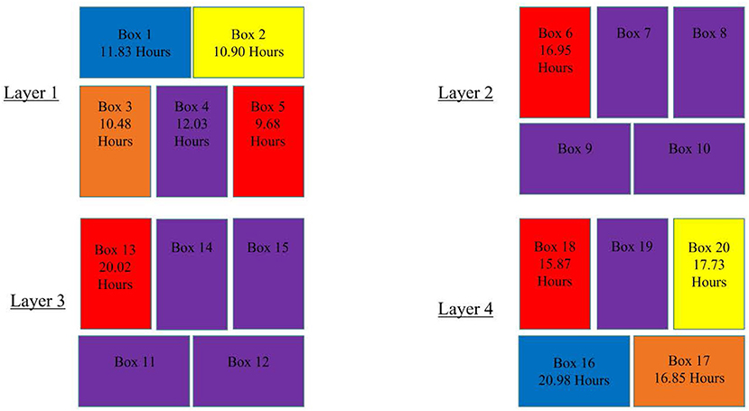
Figure 6. Cross sections of 4 layers of palletized boxes of chicken breasts with time required for each box to reach 4°C.

Thermal images

Thermal imaging is a quick and non-destructive method to measure temperature as the user can take an image from a distance (Vadivambal and Jayas, 2011). The technology has already proven to be useful in a variety of agricultural appliations such as determining food grain quality, detecting bruises on apples and grape decay (Varith et al., 2003; Nanje Gowda and Alagusundaram, 2013; Ding et al., 2017). Perhaps loading docks or cold storage facilities could benefit in the investment in thermal imaging cameras because it will aide in the decision making process of rotating their product onto shelves. Images in Figures 7, 8 show the immediate and long term impacts of cyclically removing the pallet of chicken breast from the walk-in cooler. Images shown in Figure 7 were taken less than 5 min after the pallet was pulled out of the cooler for the first time. The darker colors in the image (Figure 7) show where the pallet is the coldest and the lighter colors show where it is the hottest. The center of the pallet (layers 2 and 3) shows darker purples and blues indicating colder areas (Figure 7). The outside edges have already demonstrated lighter colors (hotter temperatures) after only 5 min of TA. Figure 8 demonstrates the thermal image of the the same pallet after it experienced six TA cycles and is at the conclusion of the 24-h TA experiment. Images in Figure 8 show most of the pallet is reddish yellow indicating the boxes, although had experienced 4°C for every alternate 2-h, did warm up and may ultimately affect the product. After 24 h of TA, thermal imaging shows heterogeneity in box temperatures based on location exemplified by the darker colors (colder temperatures) still visible in the central regions while yellow-red on the preipheral boxes (higher temperature). The results of thermal images (Figures 7, 8) are consistent with the results of the temperature profiles (Figures 2–5). In other words, layers 1 and 4 of the pallet are hotter than layers 2 and 3, and the interior boxes appear to be cooler than the perimeter boxes. Also, it is important to note that previous research has demonstrated that thermal imaging may be affected by the types of covers on products (Badia-Melis et al., 2017). Our research indicates that thermal imaging can be incorporated in cold chains especially to rapidly identify the TA without having to invest in expensive time/temperature recording devices.

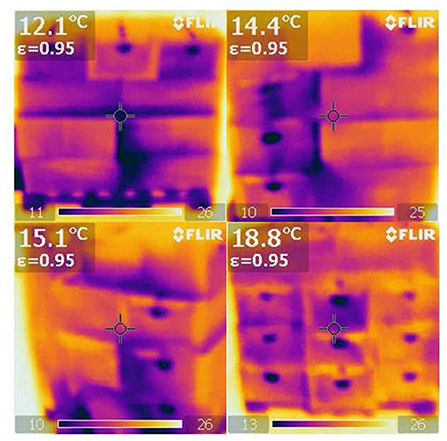
Figure 7. Thermal images of all sides of a pallet of chicken breasts immediately after being removed from a walk-in cooler (4°C).

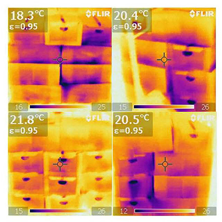
Figure 8. Thermal images of all sides of a pallet of chicken breasts after 24 h of cyclic TA (2 h at 4°C then 2 h at 25°C).

Microbiological spoilage

TA of the raw perishable poultry meat can initiate microbial growth ultimately affecting the shelf-life of the product. Experiments were conducted to determine the microbial populations (APC and PSY) on chicken at 0 and 24 h of TA. Microbial populations (APC and PSY) were similar when sampled at hour 0 and hour 24 of TA. For APC and PSY, the results were 2.2 and 2.8 log CFU/ml for 0 h of TA, respectively. After 24 h of TA the results were 2.0 to 2.4 log CFU/ml for APC and PSY, respectively. The lack of bacterial growth is likely because the TA conditions used in the study were not severe enough to cause the bacteria to immediately enter log phase. However, microbial population differences are visible when the TA and control filets were analyzed for shelf-life (Figures 9, 10). The results of both the APC and PSY show a difference in shelf-life of ~2 days between TA and control filets (Figures 9, 10). The APC and PSY of the TA and control filets reached spoilage (7 logs CFU/ml) after ~4.5 vs. 7 days (Figure 9) and 3.75 vs. 5.25 days (Figure 10), respectively. When values were compared for the sampling days of the shelf-life experiment, only day 4 was significantly different (p < 0.05) for both APC and PSY. Many similar bacterial studies have been completed with similar results (i.e., TA leads to increased bacterial growth). However, the temperatures and durations of abuse vary between studies. A study by Senter et al. (2000) found that holding chicken meat samples at a temperature of 13°C for 48 h had similar APC results to their TA scenario (3 days at 4°C then 1 day at 13°C then 1 day at 4°C). Senter et al. (2000) reported APC values of 8.19 and 9.48 log CFU/ml for the 13°C and TA scenarios, respectively. Similarly, Casanova et al. (2021) demonstrated that exposing inoculated chicken breast (Salmonella choleraesuis and Staphylococcus aureus) to 15°C for 2 h before 20 or 25°C for 10 h and finally storage at 5°C reduced the shelf-life of raw chicken from 12 days to 12 h. Ghollasi-Mood et al. (2016) exposed chicken to 4°C, 10°C, and 15°C for 8 h each and found that it took ~125 h for total viable counts to reach spoilage levels under ideal storage conditions, while TA (cyclic 8 h at 0°C then 8 h at 10°C then 8 h at 15°C) chicken took ~50 h.

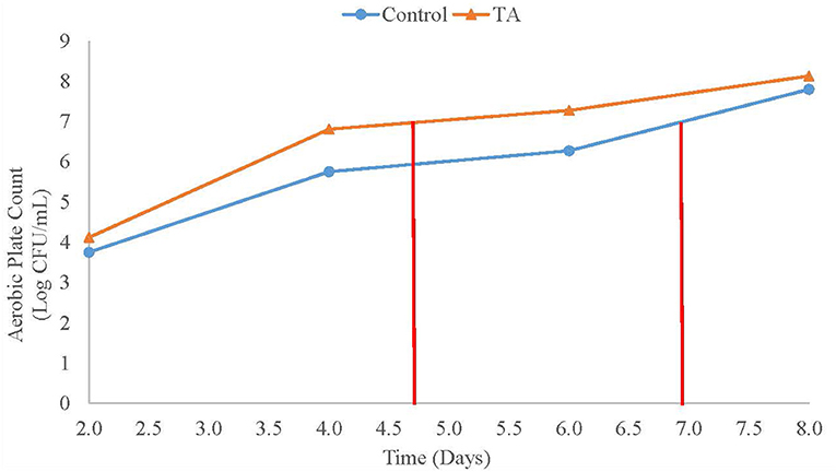
Figure 9. APC shelf-life of simulated less-than-truckload temperature abused (TA; 2 h at 4°C then 2 h at 25°C) and control chicken breast filets kept in simulated retail conditions.

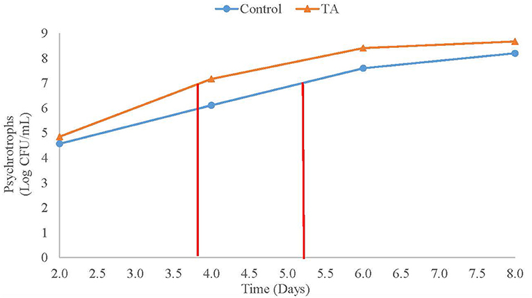
Figure 10. Psychrotroph shelf-life of simulated less-than-truckload temperature abused (TA; 2 h at 4°C then 2 h at 25°C), and control chicken breast filets kept in simulated retail conditions.

Overall, our shelf-life experiment demonstrates that TA reduces shelf-life of raw chicken breast filets compared to the non-TA control filets. If decision makers in the cold chain had knowledge of the boxes that deviated the most from control temperatures, perhaps new practices could be put in place to sell temperature sensitive products more efficiently. It is possible that a pallet received a day before may have boxes that will keep for longer than boxes on a more recently received pallet. However, under current conventions it is likely that the boxes from a pallet that arrives first will be put on display first allowing for spoilage-related food waste.

Monte Carlo and remaining shelf-life

MC simulations have been used for risk analysis in agricultural sector previously in both spoilage and food safety (Schroeder et al., 2006; Gougouli and Koutsoumanis, 2017). The method has been well documented to predict microbial counts for both spoilage microorganisms and pathogens (Schaffner et al., 2003; Zeng et al., 2014; Lau et al., 2022). For our first method the MC simulations focused on the temperatures themselves rather than predicting the microbial counts as a result of the temperatures. Table 1 shows the results of the first method using MC simulations on the 4 layers of the pallet. The table has the percent chance of each box reaching 4°C at 5 different time points during the cyclic TA (0, 6, 12, 18, and 24 h). The results of these simulations are consistent with the temperature profile results. The boxes comprising the middle layers (boxes 6–15; Table 1) have lower risks than the boxes on the top layer (boxes 1–5) and bottom layer (boxes 16–20). For layer 1, there is an incremental growth in risk of reaching the temperature “danger zone” as time goes on (Table 1). After 12 h, all boxes are at ~50% risk of having reached 4°C. Also, all layer 1 boxes have at least an 86.5% chance of reaching 4°C by the end of the experiment (24 h; Table 1). Layer 2 boxes (boxes 6–10) show a risk of less than 41% after 24 h (Table 1). However, box 6 has a 91% risk level after 24 h (Table 1) probably because of the peripheral location on the pallet but it does not explain why the other perimeter boxes were not influenced in a similar manner. MC simulations indicate that the boxes in layer 3 have the lowest overall risk for reaching 4°C (Table 1). At 12 h, layer 3 boxes were all below 11% with 4 of 5 boxes being below 4%. Only 1 box in layer 3 (box 13) crossed 50% after 24 h. Lastly, layer 4's results show 2 boxes above 10% after 12 h (Table 1). Four of the boxes in layer 4 were above 64% with the remaining box being at 47.4% after 24 h. Layer 4 boxes were relatively similar to layers 2 and 3 after 12 h. However, after 18 h, the percentages spike and results start appearing similar to those seen for layer 1 (Table 1). This is in contrast to layer 1 where there was an incremental increase in risk throughout the duration of the experiment.

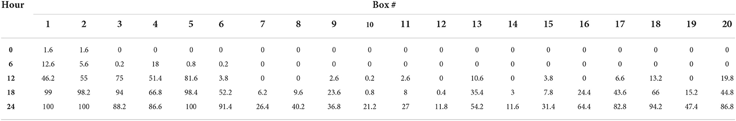
Table 1. Monte Carlo derived risk (% chance) of 4 layers of boxes of palletized chicken breasts reaching 4°C during 24 h of simulated less-than-truckload temperature abuse (2 h at 4°C, then 2 h at 25°C).

Results from the second MC method are shown in Table 2. Values for the prediction of shelf-life and risk-of-loss at 5 different TA scenarios (0, 2, 4, 6, and 8 h >4°C) are shown. The risk-of-loss increases dramatically after 6 h at >4°C (17.8%) and reached a maximum of 43.8% after 8 h >4°C. Also, shelf-life reduction increased by ~10% every additional 2 h spent at >4°C with a maximum value of 42.4% after 8 h. Lastly, the shelf-life decreased by ~3 days if filet temperature was > 4°C of rover 8 h (Table 2). MC simulation method has been used to predict shelf-life of various perishable products (Hutter et al., 2001; Schaffner et al., 2003; Giannakourou and Taoukis, 2019) including various foods (Ndraha et al., 2019; Lau et al., 2022) and pharmaceuticals (Su et al., 1994; Waterman et al., 2007). However, there are not many studies completed using MC to estimate the shelf-life of poultry. The information provided by this study and others completed previously demonstrates the complexity associated with the TA that might occur in the supply chain and why more intense temperature monitoring is needed. Perhaps a retailer could have a program already in place at the store and have the temperature history uploaded via other technologies (e.g., RFID) allowing the retailer to take advantage of the information at their disposal. Once this data is observed, the managers could easily and quickly make the most beneficial decision regarding product spoilage. Having simulations or predictive models at their disposal would allow the end user in the cold chain to make decisions without having to have an in depth understanding of microbiology. There would be no microbiological sampling involved, and it would not be necessary to have a lab to perform tests on the samples to determine the remaining shelf-life. The risk-of-loss predictions via MC methods indicate that ~44% of chicken breast filets will have a shelf-life of less than 4 days after 8 h >4°C. This method is assuming a retailer will be unable to sale product fast enough once a minimum acceptable shelf-life is reached. Therefore, the product would have to be discarded leading to food waste. In this experiment, 4 days was chosen, but the method could be altered to predict risk-of-loss at a different value for minimum shelf-life. The significance of a 44% loss becomes evident when observing the financial impact. If a pallet of chicken breasts weighs 1,000 pounds, 440 pounds could potentially be wasted. According to the United States Department of Agriculture (2022b), the price of tray packed chicken breasts is $3.06/pound. Therefore, 1 pallet could result in a financial loss of $1,346.40 if 8 h of LTL TA occurs. This highlights the need for a reliable prediction method to mitigate this food waste and associated financial loss.

Table 2. Monte Carlo derived shelf-life predictions for cyclically temperature abused (TA; 2 h at 4°C then 2 h at 25°C) chicken breasts filets determined by time (h) spent above 4°C.

Conclusion

The last mile presents challenges to cold chain management in LTL scenarios. However, limited research has been conducted on the impact of LTL TA at the pallet level of perishable goods. Our study demonstrates the heterogeneity in temperature profile of different boxes on the pallet with or at different layers and the need to use time/temperature data to understand the potential spoilage risks of each box. MC simulations demonstrated an increased risk to reach abuse level temperatures in the boxes located on the top and bottom layers (layers 1 and 4) of the pallet with the top layer being the highest risk (>86%) after 24 h. Lastly, shelf-life and risk-of-loss predictions were completed. After 8 h of exposure to temperatures >4°C, the risk-of-loss reaches nearly 44%, and shelf-life reduces from 7.2 days to 4.1 days. This study demonstrates how a “break” in cold chain can influence the shelf-life at the retail level. Simulations can be useful tools for managers when deciding how to treat their stock of temperature sensitive products, and they can allow them to more accurately judge which products to sell first.

In the future, more research is needed in last mile TA with more scenarios regarding the duration and levels of TA are needed. Also, merging new technologies into similar experiments will be essential. For example, the use of RFID technology to record temperatures is a more realistic way of collecting TA data in the cold chain. Time/temperature data collection with RFID combined with cloud computing would aid in real-time prediction of remaining shelf-life as the product is moving through the supply chain and help in better decision making about the product prior to its arrival at the retail store.

Data availability statement

The raw data supporting the conclusions of this article will be made available by the authors, without undue reservation.

Author contributions

CH conducted research and wrote manuscript. LG helped with experimental design and manuscript review. AS helped with data analysis. T-SH helped with experimental design and is a subject matter expert on Food Safety and Food Microbiology. SR helped with experimental design and is a subject matter expert on Supply Chain Management. JC provided knowledge on the FLIR infrared camera. AM obtained funding and performed manuscript review. All authors contributed to the article and approved the submitted version.

Conflict of interest

The authors declare that the research was conducted in the absence of any commercial or financial relationships that could be construed as a potential conflict of interest.

Publisher's note

All claims expressed in this article are solely those of the authors and do not necessarily represent those of their affiliated organizations, or those of the publisher, the editors and the reviewers. Any product that may be evaluated in this article, or claim that may be made by its manufacturer, is not guaranteed or endorsed by the publisher.

References

Aljohani, K., and Thompson, R. G. (2020). An examination of last mile delivery practices of freight carriers servicing business receivers in inner-city areas. Sustainability 12, 2837. doi: 10.3390/su12072837
Badia-Melis, R., Emond, J. P., Ruiz-García, L., Garcia-Hierro, J., and Robla Villalba, J. I. (2017). Explorative study of using infrared imaging for temperature measurement of pallet of fresh produce. Food Control. 75, 211–219. doi: 10.1016/j.foodcont.2016.12.008
Casanova, C. F., de Souza, M. A., Fisher, B., Colet, R., Marchesi, C. M., Zeni, J., et al. (2021). Bacterial growth in chicken breast fillet submitted to temperature abuse conditions. Food Sci. Technol. 42. doi: 10.1590/fst.47920
Chen, Z., and Meng, J. (2021). Persistence of salmonella enterica and enterococcus faecium NRRL B-2354 on baby spinach subjected to temperature abuse after exposure to sub-lethal stresses. Foods 10, 2141. doi: 10.3390/foods10092141
Curto, J. P., and Gaspar, P. D. (2021). Traceability in food supply chains: review and SME focused analysis. AIMS Agric. Food. 6, 679–707. doi: 10.3934/agrfood.2021041
de Frias, J. A., Luo, Y., Zhou, B., Zhang, B., Ingram, D. T., Vorst, K., et al. (2020). Effect of door opening frequency and duration of an enclosed refrigerated display case on product temperatures and energy consumption. Food Control. 111, 107044. doi: 10.1016/j.foodcont.2019.107044
Deutsch, Y., and Golany, B. (2018). A parcel locker network as a solution to the logistics last mile problem. Int. J. Prod. Res. 56, 251–261. doi: 10.1080/00207543.2017.1395490
Ding, L., Dong, D., Jiao, L., and Zheng, W. (2017). Potential using of infrared thermal imaging to detect volatile compounds released from decayed grapes. PLoS ONE 6, e0180649. doi: 10.1371/journal.pone.0180649
do Nascimento Nunes, M. C., Nicometo, M., Emond, J. P., Melis, R. B., and Uysal, I. (2014). Improvement in fresh fruit and vegetable logistics quality: berry logistics field studies. Philos. Trans. A Math Phys. Eng. Sci. 372, 20130307. doi: 10.1098/rsta.2013.0307
Emenike, C. C., and Hoffman, A. J. (2014). “Perishable produce temperature profiling using intelligent telematics,” in Proceedings of the Southern Africa Telecommunication Networks and Applications Conference (SATNAC) (Port Elizabeth), 363–368.
Eslami, Z., Mahdavi, V., and Tajdar-Oranj, B. (2021). Probabilistic health risk assessment based on Monte Carlo simulation for pesticide residues in date fruits of Iran. Environ. Sci. Pollut. Res. 28, 42037–42050. doi: 10.1007/s11356-021-13542-0
FedEx (2022). What is LTL freight? Available online at: https://www.fedex.com/en-us/shipping/freight/ltl.html (accessed May 17, 2022).
Gaukler, G., Ketzenberg, M., and Salin, V. (2017). Establishing dynamic expiration dates for perishables: an application of RFID and sensor technology. Int. J. Prod. Econ. 193, 617–632. doi: 10.1016/j.ijpe.2017.07.019
Getahun, S., Ambaw, A., Delele, M., Meyer, C. J., and Opara, U. L. (2017). Analysis of airflow and heat transfer inside fruit packed refrigerated shipping container: part I–model development and validation. J. Food Eng. 203, 58–68. doi: 10.1016/j.jfoodeng.2017.02.010
Ghollasi-Mood, F., Mohsenzadeh, M., Housaindokht, M. R., and Varidi, M. (2016). Microbial and chemical spoilage of chicken meat during storage at isothermal and fluctuation temperature under aerobic conditions. Iran J. Vet Sci. Technol. 1, 38–46. doi: 10.22067/veterinary.v8i1.54563
Giannakourou, M. C., Koutsoumanis, K., Nychas, G. J. E., and Taoukis, P. S. (2001). Development and assessment of an intelligent shelf-life decision system for quality optimization of the food chill chain. J. Food Prot. 64, 1051–1057. doi: 10.4315/0362-028X-64.7.1051
Giannakourou, M. C., and Taoukis, P. S. (2019). Meta-analysis of kinetic parameter uncertainty on shelf-life prediction in the frozen fruits and vegetable chain. Food Eng. Rev. 11, 14–28. doi: 10.1007/s12393-018-9183-0
Global Cold Chain Alliance (2020). About The Cold Chain. Available online at: https://www.gcca.org/about/about-cold-chain (accessed June 8, 2022).
Godwin, S. L., Chen, F. C., and Stone, R. (2012). Avoiding The Food “Danger Zone” When It Is Hot Outside. Extension Publications, 20. Available online at: https://digitalscholarship.tnstate.edu/extension/20?utm_source=digitalscholarship.tnstate.edu%2Fextension%2F20andutm_medium=PDFandutm_campaign=PDFCoverPages
Gougouli, M., and Koutsoumanis, K. P. (2017). Risk assessment of fungal spoilage: a case study of Aspergillus niger on yogurt. Food Microbiol. 65, 264–273. doi: 10.1016/j.fm.2017.03.009
Grunow, M., and Piramuthu, S. (2013). RFID in highly perishable food supply chains–remaining shelf-life to supplant expiry date? Int. J. Prod. Econ. 146, 717–727. doi: 10.1016/j.ijpe.2013.08.028
Hertog, M. L., Uysal, I., McCarthy, U., Verlinden, B. M., and Nicolaï, B. M. (2014). Shelf-life modelling for first-expired-first-out warehouse management. Philos. Trans. A Math Phys. Eng. Sci. 372, 20130306. doi: 10.1098/rsta.2013.0306
Hutter, J. C., Long, M. C., Do Luu, H. M., and Schroeder, L. W. (2001). Prediction of the shelf-life of cellulose acetate hemodialyzers by Monte Carlo simulation. ASAIO J. 47, 522–527. doi: 10.1097/00002480-200109000-00025
Jedermann, R., Ruiz-Garcia, L., and Lang, W. (2009). Spatial temperature profiling by semi-passive RFID loggers for perishable food transportation. Comput. Electron. Agric. 65, 145–154. doi: 10.1016/j.compag.2008.08.006
Jeong, J., Chon, J. W., Kim, H., Song, K. Y., and Seo, K. H. (2018). Risk assessment for salmonellosis in chicken in South Korea: the effect of Salmonella concentration in chicken at retail. Korean J. Food Sci. Anim. Resour. 38, 1043. doi: 10.5851/kosfa.2018.e37
Kadigi, I. L., Mutabazi, K. D., Philip, D., Richardson, J. W., Bizimana, J. C., Mbungu, W., et al. (2020). An economic comparison between alternative rice farming systems in tanzania using a monte carlo simulation approach. Sustainability 12, 6528. doi: 10.3390/su12166528
Labuza, T. P., and Fu, B. I. N. (1995). Use of time/temperature integrators, predictive microbiology, and related technologies for assessing the extent and impact of temperature abuse on meat and poultry products. J. Food Saf. 15, 201–227. doi: 10.1111/j.1745-4565.1995.tb00134.x
Lau, S., Trmcic, A., Martin, N. H., Wiedmann, M., and Murphy, S. I. (2022). Development of a Monte Carlo simulation model to predict pasteurized fluid milk spoilage due to post-pasteurization contamination with gram-negative bacteria. J. Dairy Sci. 3, 1978–1998. doi: 10.3168/jds.2021-21316
Leinonen, I., Williams, A. G., Wiseman, J., Guy, J., and Kyriazakis, I. (2012). Predicting the environmental impacts of chicken systems in the United Kingdom through a life cycle assessment: egg production systems. Poult. Sci. 91, 26–40. doi: 10.3382/ps.2011-01635
Maeda, E. E., Pellikka, P., and Clark, B. J. (2010). Monte Carlo simulation and remote sensing applied to agricultural survey sampling strategy in Taita Hills, Kenya. Afr. J. Agric. Res. 5, 1647–1654. doi: 10.5897/AJAR09.011
Mendes, A., Cruz, J., Saraiva, T., Lima, T. M., and Gaspar, P. D. (2020). “Logistics strategy (FIFO, FEFO or LSFO) decision support system for perishable food products,” in 2020 International Conference on Decision Aid Sciences and Application (DASA) (Sakheer), 173–178. doi: 10.1109/DASA51403.2020.9317068
Mirzaee, M., and Bishop, C. F. H. (2009). The packaging implications of the 'last mile of the strawberry supply chain'. VI International Postharvest Symposium 877, 967–972. doi: 10.17660/ActaHortic.2010.877.130
Nanje Gowda, N. A., and Alagusundaram, K. (2013). Use of thermal imaging to improve the food grains quality during storage. Int. J. Agric. Res. 7, 34–41.
National Chicken Council (2022a). Per Capita Consumption of Poultry and Livestock, 1965 to Forecast 2022, in Pounds. Available online at: https://www.nationalchickencouncil.org/about-the-industry/statistics/per-capita-consumption-of-poultry-and-livestock-1965-to-estimated-2012-in-pounds/ (accessed June 5, 2022).
National Chicken Council (2022b). Wholesale and Retail USDA Prices for Chicken, Beef, and Pork. Available online at: https://www.nationalchickencouncil.org/statistic/prices-chicken-beef-pork/ (accessed June 10, 2022).
Ndraha, N., Hsiao, H. I., Vlajic, J., Yang, M. F., and Lin, H. T. V. (2018). Time-temperature abuse in the food cold chain: review of issues, challenges, and recommendations. Food Control. 89, 12–21. doi: 10.1016/j.foodcont.2018.01.027
Ndraha, N., Sung, W. C., and Hsiao, H. I. (2019). Evaluation of the cold chain management options to preserve the shelf-life of frozen shrimps: a case study in the home delivery services in Taiwan. J. Food Eng. 242, 21–30. doi: 10.1016/j.jfoodeng.2018.08.010
Oscar, T. P. (2009). Predictive model for survival and growth of Salmonella Typhimurium DT104 on chicken skin during temperature abuse. J. Food Prot. 72, 304–314. doi: 10.4315/0362-028X-72.2.304
Özkaya, E., Keskinocak, P., Joseph, V. R., and Weight, R. (2010). Estimating and benchmarking less-than-truckload market rates. Transp. Res. E: Logist. Transp. Rev. 5, 667–682. doi: 10.1016/j.tre.2009.09.004
Pikora, M., Trzaska, K., and Ponder, A. (2021). Assessment of the impact of the functioning of the FIFO on the occurrence of organic products with an exceeded use-by date. Environ. Prot. Nat. Resou. 32, 29–36. doi: 10.2478/oszn-2021-0012
Rai, A., Sun, J., and Tassou, S. A. (2019). Numerical investigation of the protective mechanisms of air curtain in a refrigerated truck during door openings. Energy Procedia. 161, 216–223. doi: 10.1016/j.egypro.2019.02.084
Raychaudhuri, S. (2008). “Introduction to monte carlo simulation,” in 2008 Winter Simulation Conference (Miami, FL: IEEE), 91–100. doi: 10.1109/WSC.2008.4736059
Reddy, N. R., Villanueva, M., and Kautter, D. A. (1995). Shelf life of modified-atmosphere-packaged fresh tilapia fillets stored under refrigeration and temperature-abuse conditions. J. Food Prot. 58, 908–914. doi: 10.4315/0362-028X-58.8.908
Rezeki, D. S., Girsang, E., Silaen, M., and Nasution, S. R. (2022). Evaluation of drug storage using FIFO/FEFO methods in Royal Prima Medan Hospital pharmacy installation. IJHP 2, 9–17. doi: 10.51601/ijhp.v2i1.8
Rico-Contreras, J. O., Aguilar-Lasserre, A. A., Méndez-Contreras, J. M., López-Andrés, J. J., and Cid-Chama, G. (2017). Moisture content prediction in poultry litter using artificial intelligence techniques and Monte Carlo simulation to determine the economic yield from energy use. J. Environ. Manage. 202, 254–267. doi: 10.1016/j.jenvman.2017.07.034
Rogers, H. B., Brooks, J. C., Martin, J. N., Tittor, A., Miller, M. F., Brashears, M. M., et al. (2014). The impact of packaging system and temperature abuse on the shelf life characteristics of ground beef. Meat Sci. 97, 1–10. doi: 10.1016/j.meatsci.2013.11.020
Schaffner, D. W., McEntire, J., Duffy, S., Montville, R., and Smith, S. (2003). Monte Carlo simulation of the shelf-life of pasteurized milk as affected by temperature and initial concentration of spoilage organisms. Food Prot. Trends. 12, 1014–1021.
Schroeder, C. M., Latimer, H. K., Schlosser, W. D., Golden, N. J., Marks, H. M., Coleman, M. E., et al. (2006). Overview and summary of the Food Safety and Inspection Service risk assessment for Salmonella Enteritidis in shell eggs, October 2005. Foodborne Pathog. Dis. 4, 403–412. doi: 10.1089/fpd.2006.3.403
Senter, S. D., Arnold, J. W., and Chew, V. (2000). APC values and volatile compounds formed in commercially processed, raw chicken parts during storage at 4 and 13 C and under simulated temperature abuse conditions. J. Sci. Food Agric. 80, 1559–1564. doi: 10.1002/1097-0010(200008)80:10%3C1559::AID-JSFA686%3E3.0.CO;2-8
Shu, Y., Shin, K. G., He, T., and Chen, J. (2015). “Last-mile navigation using smartphones,” in Proceedings of the 21st Annual International Conference on Mobile Computing and Networking (Paris), 512–524. doi: 10.1145/2789168.2790099
Skawińska, E., and Zalewski, R. I. (2022). Economic impact of temperature control during food transportation—a COVID-19 perspective. Foods 11, 467. doi: 10.3390/foods11030467
So, J. H., Joe, S. Y., Hwang, S. H., Jun, S., and Lee, S. H. (2021). Analysis of the temperature distribution in a refrigerated truck body depending on the box loading patterns. Foods 10, 2560. doi: 10.3390/foods10112560
Su, X., Wan Po, A., and Yoshioka, S. (1994). Predicting shelf-lives of pharmaceutical products: Monte Carlo simulation using the simulation package SIMAN. J. Therm. Anal. Calorim. 41, 713–724. doi: 10.1007/BF02549344
Sukasih, E., Apriyanto, G., and Firdiansjah, A. (2020). Drug inventory management in financial perspectives on pharmacy installations. IOSR-JBM 22, 54–61. doi: 10.9790/487X-2208035461
Tassou, S. A., De-Lille, G., and Ge, Y. T. (2009). Food transport refrigeration–approaches to reduce energy consumption and environmental impacts of road transport. Appl. Therm. Eng. 29, 1467–1477. doi: 10.1016/j.applthermaleng.2008.06.027
United Nations (2022a). Global Issues Population. Available online at: https://www.un.org/en/global-issues/population (accessed on June 10, 2022).
United Nations (2022b). Global Issues Food. Available online at: https://www.un.org/en/global-issues/food (accessed on June 10, 2022).
United States Department of Agriculture (2021a). “Danger Zone” (40 °F - 140 °F). Available online at: https://www.fsis.usda.gov/food-safety/safe-food-handling-and-preparation/food-safety-basics/danger-zone-40f-140f (accessed on December 31, 2021).
United States Department of Agriculture (2022a). Food Waste FAQs. Available online at: https://www.usda.gov/foodwaste/faqs (accessed May 17, 2022).
United States Department of Agriculture (2022b). USDA National Retail Report – Chicken. Available online at: https://www.ams.usda.gov/mnreports/pywretailchicken.pdf (accessed June 8, 2022).
United States Food Drug Administration (2021). New Era of Smarter Food Safety Blueprint. Available online at: https://www.fda.gov/food/new-era-smarter-food-safety/new-era-smarter-food-safety-blueprint (accessed on December 31, 2021).
Vadivambal, R., and Jayas, D. S. (2011). Applications of thermal imaging in agriculture and food industry-a review. Food Bioprocess. Technol. 2, 186–199. doi: 10.1007/s11947-010-0333-5
Varith, J., Hyde, G. M., Baritelle, A. L., Fellman, J. K., and Sattabongkot, T. (2003). Non-contact bruise detection in apples by thermal imaging. Innov. Food Sci. Emerg. Technol. 2, 211–218. doi: 10.1016/S1466-8564(03)00021-3
Vega, D. A. S. D. L., Lemos, P. H., Silva, J. E. A. R. D., and Vieira, J. G. V. (2021). Criteria analysis for deciding the LTL and FTL modes of transport. Gest. Prod. 28. doi: 10.1590/1806-9649-2020v28e5065
Vukina, T. (2001). Vertical integration and contracting in the US poultry sector. J. Food Distrib. Res. 32, 29–38. doi: 10.22004/ag.econ.27819
Waterman, K. C., Carella, A. J., Gumkowski, M. J., Lukulay, P., MacDonald, B. C., Roy, M. C., et al. (2007). Improved protocol and data analysis for accelerated shelf-life estimation of solid dosage forms. Pharm. Res. 24, 780–790. doi: 10.1007/s11095-006-9201-4
Wen, X., and Dickson, J. S. (2012). Survival of Campylobacter jejuni and Salmonella enterica Typhimurium in vacuum-packed, moisture-enhanced pork. J. Food Prot. 75, 576–579. doi: 10.4315/0362-028X.JFP-11-343
Winston, W. L. (2022). Introduction to Monte Carlo simulation in Excel. Available online at: https://support.microsoft.com/en-us/office/introduction-to-monte-carlo-simulation-in-excel-64c0ba99-752a-4fa8-bbd3-4450d8db16f1 (accessed June 9, 2022).
Zeng, W., Vorst, K., Brown, W., Marks, B. P., Jeong, S., Pérez-Rodríguez, F., et al. (2014). Growth of Escherichia coli O157:H7 and Listeria monocytogenes in packaged fresh-cut romaine mix at fluctuating temperatures during commercial transport, retail storage, and display. J. Food Prot. 2, 197–206. doi: 10.4315/0362-028X.JFP-13-117
Keywords: Monte Carlo, spoilage, last mile logistics, LTL, food loss, food waste, APC, psychrotrophs
Citation: Herron CB, Garner LJ, Siddique A, Huang TS, Campbell JC, Rao S and Morey A (2022) Building “First Expire, First Out” models to predict food losses at retail due to cold chain disruption in the last mile. Front. Sustain. Food Syst. 6:1018807. doi: 10.3389/fsufs.2022.1018807
Received: 15 August 2022; Accepted: 03 October 2022;
Published: 20 October 2022.
Edited by:
Samuel Ayofemi Olalekan Adeyeye, Hindustan University, IndiaReviewed by:
Charles Odilichukwu R. Okpala, Wroclaw University of Environmental and Life Sciences, PolandTobi Fadiji, Stellenbosch University, South Africa
Copyright © 2022 Herron, Garner, Siddique, Huang, Campbell, Rao and Morey. This is an open-access article distributed under the terms of the Creative Commons Attribution License (CC BY). The use, distribution or reproduction in other forums is permitted, provided the original author(s) and the copyright owner(s) are credited and that the original publication in this journal is cited, in accordance with accepted academic practice. No use, distribution or reproduction is permitted which does not comply with these terms.
*Correspondence: Amit Morey, azm0011@auburn.edu