Solar magnetic flux rope identification with GUITAR: GUI for Tracking and Analysing flux Ropes

1 Introduction

Magnetic flux ropes (MFRs) are defined as bundles of twisted magnetic field lines winding around a common axis (see, e.g., Lowder and Yeates, 2017). They are a fundamental magnetic configuration in solar physics and solar - terrestrial sciences. For example, MFRs are embedded in coronal mass ejections (CMEs; Webb and Howard, 2012), which are huge clouds of magnetized plasma released from the Sun into interplanetary space. CMEs drive a significant portion of the observed terrestrial space weather events and are thus of particular interest for the space weather community.

Near-Sun information of the presence and properties of MFRs is difficult to obtain due to the inability to routinely observe the magnetic field in the tenuous and hot corona. Therefore, magnetic field modelling is commonly employed (Wiegelmann et al., 2017) where the coronal field is extrapolated using observations from the solar surface (photosphere). In our previous work, we have developed semi-automated algorithms to extract and track MFRs from three-dimensional simulation data. Wagner et al. (2023) (referred to here as Paper I) presented an initial method to extract MFR field lines under the assumption of a perfectly circular cross-section in a given plane of the 3D simulation domain. Wagner et al. (2024) (referred to here as Paper II) presented a more general approach, incorporating mathematical morphology algorithms in favor of the perfect-circularity assumption, which led to notable improvements of the extraction and tracking procedure.

With this work, we present and publicly release GUITAR (GUI for Tracking and Analysing flux Ropes), a graphical user interface (GUI), that wraps the methodology of Paper II into a user-friendly and easy-to-use application. GUITAR is intended to extract a list of source points for computing and visualizing magnetic flux rope field lines from a 3D magnetic field simulation box with a structured grid, based on 2D slices of a specified MFR proxy. Furthermore, the algorithm can be used for tracking the identified MFR in time and space. It operates in different modes, allowing the user to repeat and improve certain steps with different procedures or parameter choices.

To demonstrate the usage of GUITAR, we present here an extraction from a time-dependent magnetofrictional modeling (TMFM) simulation from AR12473 used in, e.g., Kumari et al. (2023); Wagner et al. (2023); Price et al. (2020). To identify and track the MFR in this simulation, a proxy to aid in the extraction is required. Here, we use the maps of the twist number T_w (Berger and Prior, 2006). These can be acquired, for example, by using the Q-factor code from Liu et al. (2016). It is important to point out that the applicability of GUITAR is very general, meaning that it can be combined with any kind of 2.5D or 3D magnetic field simulation (depending on the desired MFR proxy).

2 Methods

2.1 TMFM

The time-dependent magnetofrictional approach builds on the assumption that the magnetic field in the solar corona tends to evolve as driven by the velocity v that is proportional to the Lorentz-force J ×B, as in the following:

After initializing the model with a potential field solution, the magnetic field is evolved with the prescription above in a data-driven manner: the photospheric boundary condition of the model evolves according to the observed active region’s magnetogram data. Details of the modeling method are provided in Pomoell et al. (2019); Lumme et al. (2017). The exemplary analysis here is done on the TMFM dataset of active region AR12473 from Paper I and Paper II. A flux rope develops in the model as a result of the photospheric driving, and the MFR is extracted, tracked and analysed to showcase the features of GUITAR.

We use an approximation of the field line twist, as defined by Berger and Prior (2006) in Eq. 16, as proxy for the MFR, but GUITAR allows a variety of input maps (more on that in Section 4). While the basic approach here is to arrive at the desired source points for computing the MFR field lines via thresholding of the twist maps, we combine the extraction procedure with mathematical morphology algorithms, as outlined below and in Paper II in greater detail.

2.2 Mathematical morphology

In addition to choosing a suitable MFR proxy, the extraction scheme relies on mathematical morphology (MM) operations, which help to better control the extracted areas in the 2D proxy map. The basic principle of MM is the comparison of a given image with a reference object, called the structuring element (SE). For our purpose, the SE shape is a circle of user-defined size. A motivation for this choice will be given at the end of this section.

We make use of the erosion and opening algorithms for binary maps, and the morphological gradient algorithm for gray-scale images. The erosion of a binary image B by a structuring element X is given as: B ⊖ X = ⋂_x∈XB_−x, i.e., the union of the centre points of all SEs that are fully included in a binary shape. Another fundamental MM algorithm is the dilation, which is for a binary image B given as: B ⊕ X = ⋃_x∈XB_x, i.e., the union of all points of those SEs which have their center point within the binary shape. Combining dilation and erosion, we arrive at the opening algorithm: (B ⊖ X) ⊕ X. This is particularly useful to remove noise or, like in our case, to disconnect two distinct features that are connected via some thin channel or remove a sub-feature from the original contour. This is shown in an example in Figure 1, where both the erosion and the dilation of the erosion (i.e., the opening) are shown as separate contours. One can see, how this not only proves to be useful to better control the outlines of what is extracted, but disconnecting an unwanted structure from the MFR in 2D. This greatly improves the tracking in tricky cases, where multiple twisted features (not necessarily MFRs) are present, which might lead to tracking the wrong feature in subsequent frames.

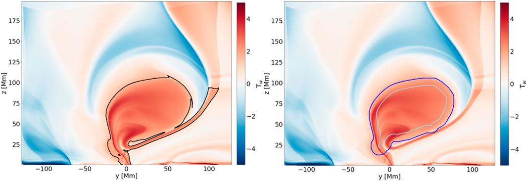
Figure 1. Sub-steps of the opening algorithm. The base image is a twist map of frame 20, with the original contour of the extraction from the T_w + ∇T_w map in black on the left. On the right, the contours of the erosion are shown in lightblue, while the dilation, which completes the opening algorithm, is shown in blue.

The morphological gradient for a gray-scale image G is the difference between the dilation and erosion, where the SE for both can be chosen freely: ∇G = (G ⊕ X₁) − (G ⊖ X₂). For gray-scale images, dilation and erosion work the following way: First the neighbouring points to each pixel are identified via the structuring element (with the pixel of interest at the centre of the SE). Subsequently, these central pixels are replaced by the supremum/infimum values of their respective neighbours to arrive at the dilated/eroded image of G. The morphological gradient proves to be useful to detect/enhance edges in an image, which we use to make our proxy maps more robust against the choice of a threshold, to ultimately identify the MFR feature.

Our choice of the SE shape (i.e., circular) results in smooth outlines in regions where these algorithms are applied. This is especially useful to retain the rather rounded contours found in the twist maps, for example, in cases where it is desired to disconnect a sub-feature from the main body in the 2D slice.

2.3 Requirements

GUITAR is written in python 3.10 and based on the tkinter library. Further necessary non-standard packages include: skimage, pyvista, diplib and cv2. To save animations, imagemagick is required as an additional software, but the code also runs without it.

The proxy maps presently need to be 2D slices of a 3D data cube. They can be read-in either .vtr- or .npz-files, although the latter is recommended if multiple time-steps should be investigated, as the procedure for reading the .vtr files is more time-consuming.

2.4 Functionalities

In its current version, GUITAR offers four different modes of operation:

1. Full extraction mode,

2. Post-processing mode,

3. Source point retrieval mode,

4. Difference map mode.

The full extraction mode (main window shown in Figure 2) contains every step from start (i.e., some map of a MFR proxy) to finish (i.e., a list of source points for the computation of the magnetic field lines) and offers an option to save the current state of the processed input maps at various points during the extraction and tracking procedure. These files can then be used as inputs to the other three modes. The post-processing mode starts from some intermediate step (a map that is at least already reduced to binary) and can be used to apply new (MM-)processings, re-track the resulting features and save a list of source points for computing the field lines, as a final step. The source-point retrieval mode can be used to change the sampling without having to go through the full extraction process or post-processing process again. It again starts from some binary input map, but skips directly to the computation of the source points list. The last mode is the difference maps mode, which enables creating difference maps from previously created binary masks of two different extractions and can be used to either save the resulting binary difference map and/or the source points, calculated from them. This is useful, e.g., if different (sub-)structures of a particular map should be visualized together or to see the difference between different choices of processing algorithms or parameters. For example, one can make an initial extraction A, and then follow-up with focusing on one particular feature B. To show both in the same field line plot without having overlapping field lines, one can create the difference map source points C, and then visualize C together with B. The desired mode can be selected in the starting-window, upon running GUITAR.

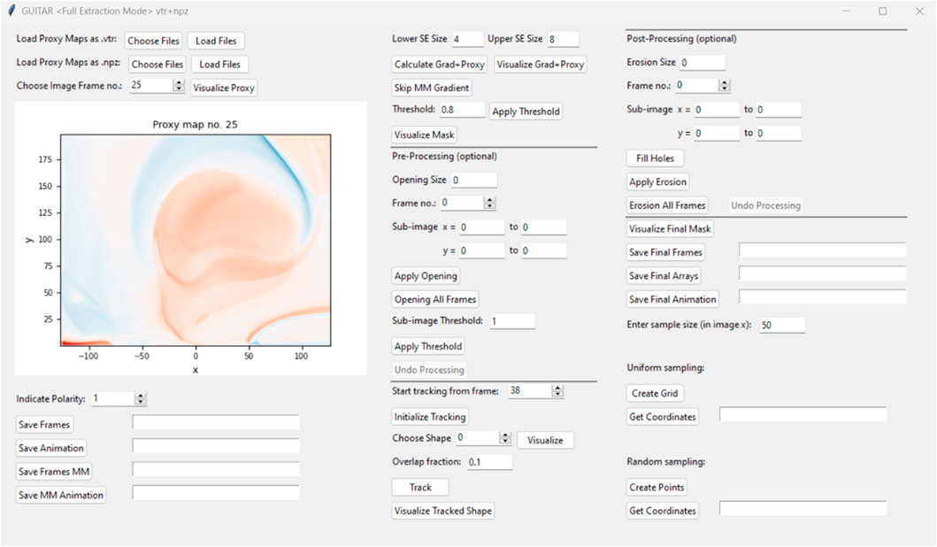
Figure 2. Main window of GUITAR.

2.5 Extraction and tracking procedure

In the following, we will briefly outline the MFR extraction and tracking (full extraction mode) using maps of T_w as flux rope proxy, computed from the simulation outlined in Sect. 2.1. The choice of the proxy parameter will only affect the preferred sign of the proxy (called “polarity” within GUITAR) and the value of the thresholds (see below), which can both be customized in the interface.

The extraction of MFR source points is facilitated by identifying high-|T_w| regions, aided by mathematical morphology (MM) algorithms. The sign of twist (helicity sign or chirality) can be specified in the corresponding spin box (1 = positive polarity, −1 = negative polarity) to exclude oppositely twisted field lines. The morphological gradient is applied to the T_w maps as a sharpening routine, where both the size of the smaller and larger SE can be customized. Then, a threshold is set to find the highly twisted regions by reducing the maps to binary masks (1 if the threshold is met, and 0 otherwise). The morphological gradient has the effect, that the outlines may appear sharper and thus makes the extraction slightly less dependent on the choice of the threshold. The possibility to fine-tune the morphological gradient further facilitates this stabilization effect.

Following the thresholding, a pre-processing step can optionally be applied before the tracking procedure. Here, the retrieved binary masks can be modified by applying the opening algorithm (cf., Section 2.2). This is a useful procedure, for example, in the case when two separate features are connected and only one of them is regarded as part of the structure that should be tracked. Applying a suitable MM opening can remove this problem as it can be used to disconnect such features for problematic frames. Furthermore, since the openings with substantial SE sizes can significantly distort the extracted outlines of the MFR cross-section, GUITAR offers to apply this procedure only in a sub-region of the image.

For the tracking of the MFR structure, GUITAR marks the four largest connected regions in each binary mask. To initialize the tracking, the user specifies the frame from which the tracking will be started (which should be the last frame in which the twisted structure can still be identified). The user then selects the region of interest out of these four high-twist regions in this frame. Subsequently, GUITAR identifies in each preceding frame a structure as being the same as the selected one, if they overlap sufficiently. The necessary overlap ratio, a number between 0 (= no overlap) and 1 (=100 percent overlap), can be defined by the user. If no sufficiently overlapping region is found, the previously identified region is kept as the current one.

After the tracking procedure, GUITAR offers an opportunity to post-process the tracked mask with MM operations (erosion or fill holes). The erosion might be useful to see into different layers of the MFR, as it (as the name suggests) erodes the extracted outlines with the size and shape of the SE. The “Fill Holes” procedure marks any non-MFR regions, which are fully enclosed by MFR-regions as MFR-regions, and thus, removes holes in the extracted areas. Next, one can proceed with the retrieval of source points, where the sampling rate as well as the sampling type (random or uniform) can be specified. Finally, the calculated points are saved as text files. These files can then be used for computing and subsequently visualizing and analysing the corresponding magnetic field lines. In our example below, we will use the VisIt visualization software to do so (Childs et al., 2012).

3 Extraction of MFR in AR12473

As a showcase of GUITAR, we use the TMFM simulation of AR12473 to perform a full extraction and, additionally, use different thresholds to access different sub-structures of the twist maps. This procedure uses all four modes of GUITAR. First, we attempt to extract the full MFR, similar to “Paper II”, thus using the default threshold of 0.8 for T_w + ∇T_w (i.e., the twist maps, sharpened by the morphological gradient). We proceed with the tracking and save the resulting binary mask for this initial extraction. Next, we extract a highly twisted sub-structure that appears from frame 10 onward by using a high threshold of 1.2 and utilizing MM operations to separate it from the main MFR-parts. We then track it through the domain and save the mask and the source points via uniform sampling (sampling rate: 60 points in image x). We note that for extracting this sub-feature, substantially more pre-processing was necessary to have a clear separation between the main MFR body and the desired sub-feature in 2D.

In the next step, we load both masks (the initial extraction and the extraction of the notably more twisted sub-feature) into the difference map mode, where we subtract the highly twisted feature from the main MFR extraction. To ensure that we have a clean mask remaining, we save it and re-open it in the post-processing mode to re-track the MFR. The tracking algorithm only follows connected features in the maps, thus, re-tracking the main MFR cleans the mask from disconnected patches that appear due to the applied processing. Next, the corresponding source points are retrieved.

We also extract another feature from the twist maps to illustrate that practically any distinct feature of the proxy maps can be extracted. As a last step, we create a sample of source points from the two main features in the source point retrieval mode, using uniform sampling and 30 points for the main MFR and 40 points for the sub-feature. The flexible sampling ensures control over how many field lines are drawn, which is helpful for visualization purposes. A comparison of the different samplings and the MFR appearance for two characteristic frames is shown in Figure 3 and an illustration of the field lines along with the substructures they originate from in the T_w-maps is shown in Figure 4.

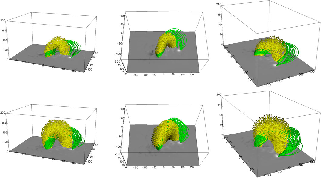
Figure 3. Field line plots, showcasing the two main substructures. Top Row: Frame 17, Bottom Row: Frame 24. The columns show different perspectives. The field lines are computed via uniform sampling with 30 points for the yellow field lines and uniform sampling with 40 points for the green field lines.

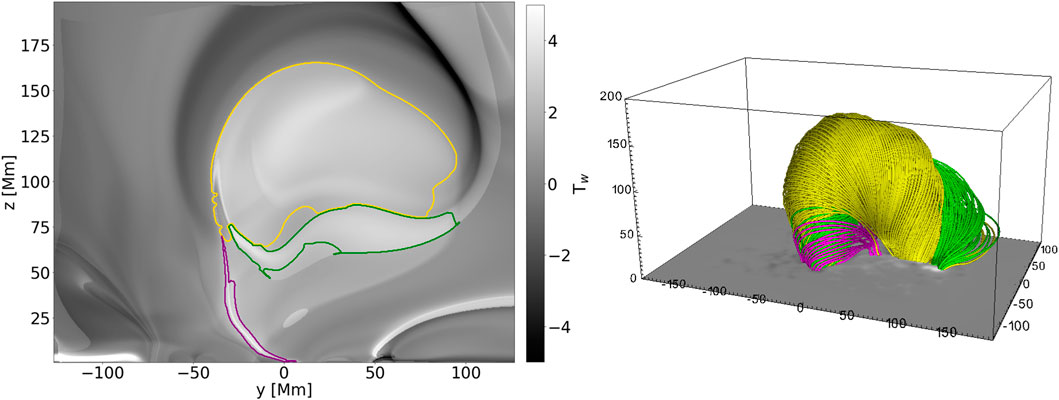
Figure 4. Illustration of the twist-substructure separation. Left: The twist map of Frame 25 in the y-z plane with the twist parameter in gray-scale and the identified substructures in differently colored contours. The selected colors match with the resulting field lines on the right (e.g., the yellow contour marks the source region for the yellow field lines, etc.). An erosion with a SE of 4 pixels has been applied to the yellow contours to ensure that they do not overlap with the green ones. Right: The corresponding field lines as they appear from the extracted areas on the left with uniform sampling, using 60 points in x, with the different features having different field line colors.

Visually, the main MFR body (yellow field lines) appears as a strikingly coherent bundle of twisted magnetic field lines. The sub-feature extracted from the twist maps, visualized with green field lines, is a distinctly different set of field lines. This becomes apparent from their different photospheric connectivity: They partially connect to another spot of strong positive polarity magnetic field in the photosphere, while being rooted in the same negative polarity region at the other footpoint. Although the green field lines appear less coherent at the positive polarity footpoint, they stay within the bounding box and wrap very coherently around the set of yellow field lines. This behaviour can be seen throughout most of the evolution of the MFR, as the late-stage snapshots in Figures 3, 4 show.

Furthermore, we highlight the difference between the two MFR structures of Figure 3 by showing the evolution of their respective average twist in Figure 5, where the colors correspond to the colors of the field lines in Figures 3, 4. The average twists are indeed significantly different (which is expected due to the different thresholds), but also their evolution deviates for most of simulation time: Feature 1 (corresponding to the yellow field lines) first shows average T_w values below 1, and picks up around frame 20, where it rises to values of about 1.05. Feature 2 on the other hand (green field lines) shows an initial peak of average twist after its formation, with T_w values of about 1.2. After a rather sharp dip to values in between 1.05 and 1.1, it recovers its initial level of T_w ≈ 1.2 and continues rising from there until the end of the simulation.

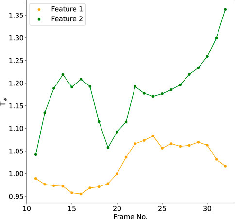
Figure 5. Twist evolution of the main MFR body (yellow field lines of Figure 3) and the second identified feature (green field lines of Figure 3).

4 Discussion

The presented MFR extraction GUI, GUITAR, wraps a number of useful image processing tools into an easy-to-use interface. The implementation leaves the freedom to use different MFR proxies and focuses on identifying and tracking the MFR features in 2D maps and compute the source points from it. The different operation modes help to re-do certain sub-steps of previous extractions to aid in arriving at an ideal set of source points. The difference map feature cannot only be used to extract, track and visualize different substructures of the twist maps, but also to visualize the effect of different MM operations. For example, one may attempt a quick extraction and then apply different processing algorithms and different parameter choices. Subsequently, one could visualise the field lines of the original extraction together with those that the difference map yields. This uncovers the field lines that are removed/added by different processing procedures. This can greatly aid in improving the extraction in terms of choosing the optimal processing approach and set of parameters, or for estimating the robustness of the tracking. For this purpose, the synergy between the post-processing mode and the difference map mode proves to be very useful.

In the presented example, the scheme is applied to a TMFM simulation of AR12473 (same as, e.g., Paper I and Paper II), where different substructures in the twist maps could be identified. These substructures appear in the modelling data as distinctly different sets of field lines, as highlighted in Figure 3 with differently colored field lines. Figure 4 in particular shows for Frame 25, the identified source regions together with the twist map, highlighting how these different sub-features appear visually distinct. Furthermore, the different photospheric connectivity of the footpoints and the different evolution of the field lines’ twist values (cf., Figure 5) supports the assumption that these are different flux rope systems. Taking a closer look at the positive polarity footpoint, we observe this very clearly for the yellow and green field lines, though the whole footpoint region seems to grow with time, where the yellow field lines migrate to the second spot of positive polarity over time (cf. Top and bottom panels in Figures 3, 4). With this, both features (yellow and green field lines) seem to slowly merge in the later stages. This example highlights that in some more complex cases, we observe not only one flux rope, but rather a system of flux ropes, where we need to disentangle the relevant sub-features to really understand the full evolution of the system (in this case, for example, this may be relevant in better understanding the footpoint movement).

While GUITAR is primarily designed and used for solar magnetic flux rope identification and tracking, the methodology provides the freedom to use any kind of input map, which may allow many different applications. The applications are foreseen to extent to other fields as well, as the presented toolset involves identification and tracking a connected image feature in essence. GUITAR will undergo continuous development, especially aiming at adding useful features and broadening the applicability to as many types of datasets as possible, though with the focus remaining on magnetic flux rope extraction.

Data availability statement

The datasets presented in this study can be found in online repositories. The names of the repository/repositories and accession number(s) can be found in the article/Supplementary material. Code available at: https://github.com/wandi0909/GUITAR.

Author contributions

AW: Conceptualization, Data curation, Formal Analysis, Investigation, Methodology, Resources, Software, Validation, Visualization, Writing–original draft, Writing–review and editing. DP: Conceptualization, Methodology, Resources, Software, Supervision, Validation, Visualization, Writing–review and editing. SB: Conceptualization, Methodology, Validation, Writing–review and editing. JP: Conceptualization, Methodology, Resources, Supervision, Writing–review and editing. SP: Funding acquisition, Supervision, Validation, Visualization, Writing–review and editing. EK: Conceptualization, Funding acquisition, Methodology, Project administration, Supervision, Validation, Writing–review and editing.

Funding

The author(s) declare financial support was received for the research, authorship, and/or publication of this article. This work is part of the SWATNet project funded by the European Union’s Horizon 2020 research and innovation programme under the Marie Skłodowska-Curie grant agreement No. 955620. DP acknowledges Horizon 2020 grant No 101004159 (SERPENTINE). JP acknowledges Academy of Finland project SWATCH (343581). We acknowledge the Finnish Centre of Excellence in Research of Sustainable Space (Academy of Finland grant number 312390). SP acknowledges support from the projects C14/19/089 (C1 project Internal Funds KU Leuven), G.0B58.23N and G.0025.23N (WEAVE) (FWO-Vlaanderen), 4000134474 (SIDC Data Exploitation, ESA Prodex-12), and Belspo project B2/191/P1/SWiM.

Acknowledgments

AW acknowledges the help of Joshua Hoffer for testing and adapting GUITAR for usage on Ubuntu. We acknowledge Teresa Barata, Robertus Erdélyi, Orlando Oliveira and Ricardo Gafeira who contributed to building the methodology.

Conflict of interest

The authors declare that the research was conducted in the absence of any commercial or financial relationships that could be construed as a potential conflict of interest.

Publisher’s note

All claims expressed in this article are solely those of the authors and do not necessarily represent those of their affiliated organizations, or those of the publisher, the editors and the reviewers. Any product that may be evaluated in this article, or claim that may be made by its manufacturer, is not guaranteed or endorsed by the publisher.

References

Berger, M. A., and Prior, C. (2006). The writhe of open and closed curves. J. Phys. A Math. General 39, 8321–8348. doi:10.1088/0305-4470/39/26/005
Childs, H., Brugger, E., Whitlock, B., Meredith, J., Ahern, S., Pugmire, D., et al. (2012). “Visit: an end-user tool for visualizing and analyzing very large data,” in High performance visualization–enabling extreme-scale scientific insight, 357–372. doi:10.1201/b12985
Kumari, A., Price, D. J., Daei, F., Pomoell, J., and Kilpua, E. K. J. (2023). Effects of optimisation parameters on data-driven magnetofrictional modelling of active regions. Sol. Stellar Astrophysics 675, A80. doi:10.1051/0004-6361/202244650
Liu, R., Kliem, B., Titov, V. S., Chen, J., Wang, Y., Wang, H., et al. (2016). Structure, stability, and evolution of magnetic flux ropes from the perspective of magnetic twist. Am. Astronomical Soc. 818, 148. doi:10.3847/0004-637X/818/2/148
Lowder, C., and Yeates, A. (2017). Magnetic flux rope identification and characterization from observationally driven solar coronal models. Am. Astronomical Soc. 846, 106. doi:10.3847/1538-4357/aa86b1
Lumme, E., Pomoell, J., and Kilpua, E. K. J. (2017). Optimization of photospheric electric field estimates for accurate retrieval of total magnetic energy injection. Sol. Phys. 292, 191. doi:10.1007/s11207-017-1214-0
Pomoell, J., Lumme, E., and Kilpua, E. (2019). Time-dependent data-driven modeling of active region evolution using energy-optimized photospheric electric fields. Sol. Phys. 294, 41. doi:10.1007/s11207-019-1430-x
Price, D. J., Pomoell, J., and Kilpua, E. K. J. (2020). Exploring the coronal evolution of AR 12473 using time-dependent, data-driven magnetofrictional modelling. A&A 644, A28. doi:10.1051/0004-6361/202038925
Wagner, A., Bourgeois, S., Kilpua, E. K. J., Sarkar, R., Price, D. J., Kumari, A., et al. (2024). The automatic identification and tracking of coronal flux ropes. II. New mathematical morphology-based flux rope extraction method and deflection analysis. Astronomy Astrophysics 683, A39. doi:10.1051/0004-6361/202348113
Wagner, A., Kilpua, E. K. J., Sarkar, R., Price, D. J., Kumari, A., Daei, F., et al. (2023). The automatic identification and tracking of coronal flux ropes - i. footpoints and fluxes. A&A 677, A81. doi:10.1051/0004-6361/202346260
Webb, D. F., and Howard, T. A. (2012). Coronal mass ejections: observations. Living Rev. Sol. Phys. 9, 3. doi:10.12942/lrsp-2012-3
Keywords: Sun, magnetic flux ropes, GUI, solar eruptions, modelling
Citation: Wagner A, Price DJ, Bourgeois S, Pomoell J, Poedts S and Kilpua EKJ (2024) Solar magnetic flux rope identification with GUITAR: GUI for Tracking and Analysing flux Ropes. Front. Astron. Space Sci. 11:1383072. doi: 10.3389/fspas.2024.1383072
Received: 06 February 2024; Accepted: 22 April 2024;
Published: 10 May 2024.
Edited by:
Dipankar Banerjee, Indian Institute of Astrophysics (IIA), IndiaCopyright © 2024 Wagner, Price, Bourgeois, Pomoell, Poedts and Kilpua. This is an open-access article distributed under the terms of the Creative Commons Attribution License (CC BY). The use, distribution or reproduction in other forums is permitted, provided the original author(s) and the copyright owner(s) are credited and that the original publication in this journal is cited, in accordance with accepted academic practice. No use, distribution or reproduction is permitted which does not comply with these terms.
*Correspondence: Andreas Wagner, andreas.wagner@helsinki.fi