Climatology of atmospheric solar tidal mode effects on ionospheric F₂ parameters over the American sector during solar minimum between cycles #23 and #24

1 Introduction

Atmospheric solar tides are global-scale oscillations that arise due to the rotation of the Earth concerning the Sun with periods and subperiods of a solar day (24 h). The tides are believed to be mainly excited by the absorption of solar radiation by tropospheric water vapor and stratospheric ozone (Lindzen and Chapman, 1969). In agreement with the period of the oscillation, the tides can be classified into different components, named diurnal (24 h), semidiurnal (12 h), terdiurnal (8 h), and quarter-diurnal (6 h), and present a large latitudinal variability, being more/less intense at low/middle-and-high latitudes for the diurnal mode, for example, and more/less intense at middle-and-high/low latitudes for the semidiurnal mode (Manson et al., 1989; Davis et al., 2013). The amplitudes of the terdiurnal and quarter-diurnal tides are generally small when compared to diurnal and semidiurnal tides (Hagan and Forbles, 2022); however, even so, they can help us to understand the variability of some phenomena. For example, Fontes et al. (2022) showed the influence of terdiurnal tide on sporadic E_s layer formation, while Santos et al. (2023) showed the importance of this tide mode to the hmF₂ and foF₂ variability over the Brazilian equatorial region during the solar minimum periods.

As the thermal structure of the atmosphere is strongly modulated by solar heating, the tides also can be classified between migrating and non-migrating. The migrating component is sun-synchronous, propagates westward with the subsolar point, and is directly excited by the heating of the atmosphere by solar radiation. On the other hand, the non-migrating tides are out of the subsolar point and propagate westward, eastward, or stay stationary. They are excited primarily by longitudinal differences in latent heat release from deep tropospheric convection at tropical latitudes or non-linear interactions between stationary planetary waves and the migrating tides. Both migrating and non-migrating have essential influences on the atmosphere (Hagan and Forbes, 2002; Griffith and Mitchell, 2022).

Another interesting characteristic of solar tides is related to their vertical propagation. It has been observed that tides excited in the lower atmosphere have an upward-propagating property, and their amplitude exponentially increases with height as the background atmospheric density decreases. Their maximum amplitude is observed in the mesosphere and lower thermosphere (MLT) region, between ∼90 and 150 km. The amplitudes of tidal variations in the region from the troposphere to the lower mesosphere are generally smaller than in the MLT (see, for example, Sakazaki et al., 2018). Regarding the dependence on solar activity, Andrioli et al. (2022) reported the existence of an anticorrelation between F10.7 cm solar flux and amplitudes of the semiannual oscillation of diurnal and semidiurnal tides. Using the mesospheric winds measurements registered by a meteor radar at the low latitude MLT region of Cachoeira Paulista (22.7°S; 45°W) during a period of 21 years, it was found that the amplitudes of the meridional diurnal and semidiurnal tide were in averaged 30% and 28%, respectively, more intense in solar minimum than in solar maximum. On the other hand, the amplitudes of zonal diurnal and semidiurnal tidal modes were 14% and 20%, respectively, more intense at solar minimum conditions.

It has been widely discussed that the ionospheric variability, among other reasons, can be associated with meteorological factors resulting from the upward-propagating tides, planetary waves, and gravity waves (see, for example, Mendillo et al., 1998). As mentioned by Forbes et al. (2000), these oscillations have the potential to impact the E-region conductivities, modulate the temperature and wind structure of the thermosphere, and generate electric fields through the dynamo mechanism, affecting in this way the ionosphere region (Forbes, 1996).

Forbes (2021) recently published an overview of atmosphere-ionosphere coupling by solar and lunar tides. He explained in detail that it is in the range of height between 90 and 150 km that the oscillations in tidal winds couple to the ionosphere and generate electric fields, currents, and induced magnetic fields. In the E ionospheric region, for example, tidal winds can contribute to the formation of sporadic E layers. Besides that, the nondivergence of E-region electric currents driven by the waves leads to the generation of so-called dynamo electrostatic fields that map to the F-region and redistribute the plasma in the form of E × B drifts that present the signatures of the driving waves. The uplift of ionospheric plasma at the equator to altitudes >800 km and the subsequent diffusion down the magnetic field line create a pileup of ionization around ±15°–20° magnetic latitude. This plasma redistribution phenomenon, known as Equatorial Ionospheric Anomaly (EIA), reflects the influence of nonmigrating tides. Therefore, although most tidal waves from the lower and middle atmosphere are not able to propagate into the F-region ionosphere, they can influence the distribution of F-region plasma by modulating the ionospheric E-region wind dynamo and equatorial plasma fountain (Millward et al., 2001).

Oikonomou et al. (2021) showed that the thermospheric tides could play a crucial role in the formation and dynamics of sporadic E (E_s) layers and intermediate descending layers over the European mid-latitude sector. Using the height–time–intensity technique, they verified that both layers present some periodicities that are probably induced by the semi-, quarter-, and terdiurnal thermospheric tides. Over the low latitude region, the contribution of tides to the motion of the descending layers also has been investigated [see, for example, Mathews et al. (1993)].

Yamazaki and Richmond (2013) investigated the daytime ionospheric response to upward propagating tides using the three-dimensional time-dependent model of the coupled thermosphere and ionosphere (Thermosphere-Ionosphere General Circulation Model—TIE-GCM). They verified that when tides are included in the simulations, both the E-region currents and the equatorial F-region vertical plasma drift (V_z) increased by ∼ 70%. Regarding the low-latitude ionospheric total electron content (TEC), an increase was noted, then gradually decreased to below the initial level by 15%. Such an increase was associated with the electric field induced by upward-propagating tides that enhance the daytime upward plasma transport at the magnetic equator and the subsequent downward and poleward diffusion of F-region plasma to low latitudes along the magnetic field lines. On the other hand, the gradual decrease was probably due to the enhanced equatorial plasma fountain, while the subsequent decline in the changes in the neutral composition was due to the tidal mixing of major species in the thermosphere. As mentioned by Sagawa et al. (2005), it is believed that the tidal amplitudes decay in the E-region altitudes; therefore, it is impossible that it affects the F-region directly. However, the results of Yamazaki and Richmond (2013) show evidence that most tidal waves from the lower and middle atmosphere can influence the distribution of F-region plasma by modulating the ionospheric E-region wind dynamo and equatorial plasma fountain, as mentioned above.

Santos et al. (2023) recently investigated the ionospheric variability over the Brazilian equatorial region during the minimum solar cycle periods of 1996 and 2009. Among the results presented, the authors showed that the contribution of the diurnal component to the hmF2 variability was similar in both periods and higher in the months from September to April. Regarding the semidiurnal mode, the most significant contribution was observed from April to September for both 1996 and 2009. Besides that, it was also observed that the hmF2 and foF2 terdiurnal and the semidiurnal tide components presented an opposite behavior throughout the year, with the terdiurnal hmF2/foF2 component smaller/higher than the semidiurnal component during the winter and higher/smaller for the summer period. Regarding foF2, it was observed that the higher intensity of tide components was observed for 1996, except for the 24 h component, which presented comparable results for both solar minimum periods. Besides the important contribution of the diurnal component to the foF2 variability, it highlighted the terdiurnal tide, which was higher than the semidiurnal tide for almost the entire year, except for the southern summer.

In this context, the present work is developed to investigate the impacts of solar tides on the foF₂ and hmF₂ over the American sector during the deep solar minimum of the transition between solar cycles #23 and #24. For that, it will be used the data registered by the Digisonde of twelve stations distributed in a latitude range that varies from 77°N to 55°S obtained in the Global Ionospheric Radio Observatory (GIRO) portal. It is important to emphasize that the period chosen to study is very special since it corresponds to one of the lowest solar activity of the modern era. This paper is organized into three different sections: geophysical conditions and data sets; results; discussion and conclusions.

2 Geophysical conditions and data set

This study used all the available digisonde data over the American sector during the deep solar minimum period from July 2007 to December 2010 (the transition from solar cycle #23 to #24). The parameters investigated correspond to the foF₂ and hmF₂. Figure 1 shows the geophysical and geomagnetic conditions from 2003 to 2013 based on solar index flux F10.7 [1 SFU = 10^–22 W/(m²Hz)] (Figure 1A) and Kp daily sum (Figure 1C). The red curve highlights the period chosen for our study. As indicated by the occurrence rate regarding the F10.7 index (Figure 1B) and Kp daily sum (Figure 1D), the data set used in this work was acquired in most of the cases during periods of very low solar and geomagnetic activity conditions (F10.7 < 71 SFU and Kp daily sum < 12, respectively). Although a minor geomagnetic influence exists during solar minimum cycles #23 and #24 [see, for example, Cai et al. (2021); Zhai et al. (2023)], this period is considered appropriate to our investigations because the variability of the foF2 and hmF2 due to the geomagnetic and solar changes can be minimized.

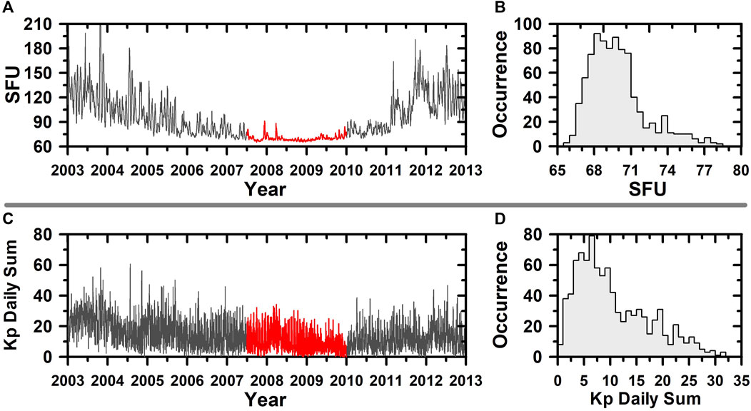
FIGURE 1. Geophysical conditions based on F10.7 cm solar flux (A) and planetary Kp index daily sum (C). On the (B) is presented a histogram of the distribution of solar activity levels during the period studied, and on (D), the same, but for the distribution of the geomagnetic activity levels. The highlighted part in red shows the period used in this work.

The digisonde data used here were automatically scaled and were obtained directly from the website https://giro.uml.edu/didbase/scaled.php. Figure 2 shows the geographic distribution of all stations studied. Table 1 gives details about them, such as code and name, as well as each station’s geographic and geomagnetic latitude and geographic longitude.

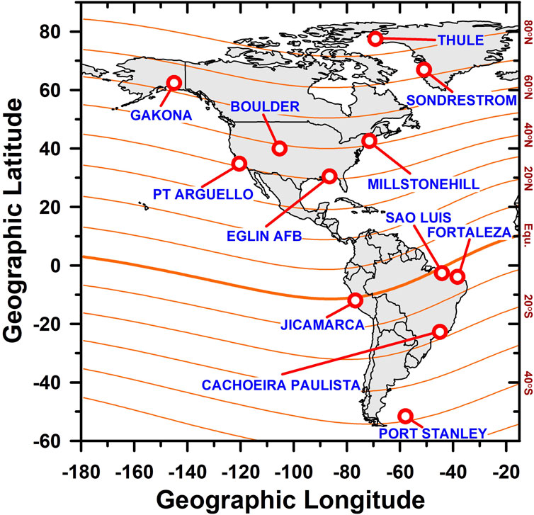
FIGURE 2. Geographic distribution of the studied stations with respect to the American Sector. The orange lines represent the geomagnetic latitude.

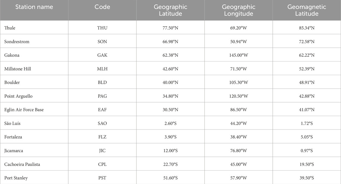
TABLE 1. Stations used in this work.

3 Results

To understand the atmospheric solar tidal mode effects on the critical frequency and the peak height of the F layer over the different localities described in Table 1, first, it was investigated these parameters’ latitudinal and seasonal variability. Afterward, the latitudinal variation of atmospheric solar tides modes on hmF2 and foF2 was studied using the same methodology proposed by Santos et al. (2023), as presented below.

3.1 Latitudinal and seasonal dependence of hmF₂ and foF₂

Figure 3 shows the latitudinal and seasonal behavior of foF₂ and hmF₂ over the twelve stations from the northern to the southern American sector (from the top to the bottom panel, respectively). In this case, it was considered the hourly average of hmF₂ and foF₂ by day of the year for the studied period. The latitudinal dependence of both parameters can be noted, with the higher intensities of frequency and height occurring in the stations near the equator. It is important to emphasize that when it is mentioned “near to the equator” or something similar, it is considered the distribution of the stations presented in Figure 1. In that figure, it is possible to note that the stations located to the south are much nearer to the geomagnetic equator than the stations located in the north. In general, over the northern latitudes (from Thule—THU to Eaglin AFB—EAF), the higher intensities of hmF₂ were observed at nighttime, mainly during the equinoxes and winter solstice. Over the Point Arguello (PAG) and EAF, for example, which are located at almost the same north geomagnetic latitude, the hmF₂ presented higher values after midnight around the equinoxes. Also, it is highlighted that the higher peak height values over the northern along the year occurred over THU and PAG. Over the stations located to the south of the geomagnetic equator, it is possible to note an increase in hmF₂ compared to the north stations. Over the Brazilian stations of São Luis (SAO) and Fortaleza (FLZ), two peaks around the equinoxes are noted, one near midday and another around sunset. This later peak is likely to the pre-reversal enhancement of the zonal electric field (∼18 LT). Over Jicamarca (JIC), peaks in the equinoxes and summer are observed with less intensity than those observed over SAO. Over Cachoeira Paulista (CPL), a low latitude station in the southern hemisphere, the hmF₂ parameter presented low values during the winter solstice and a peak during the summer at about 12 LT. It was also observed that high values of hmF₂ after midnight, except on some days around the winter.

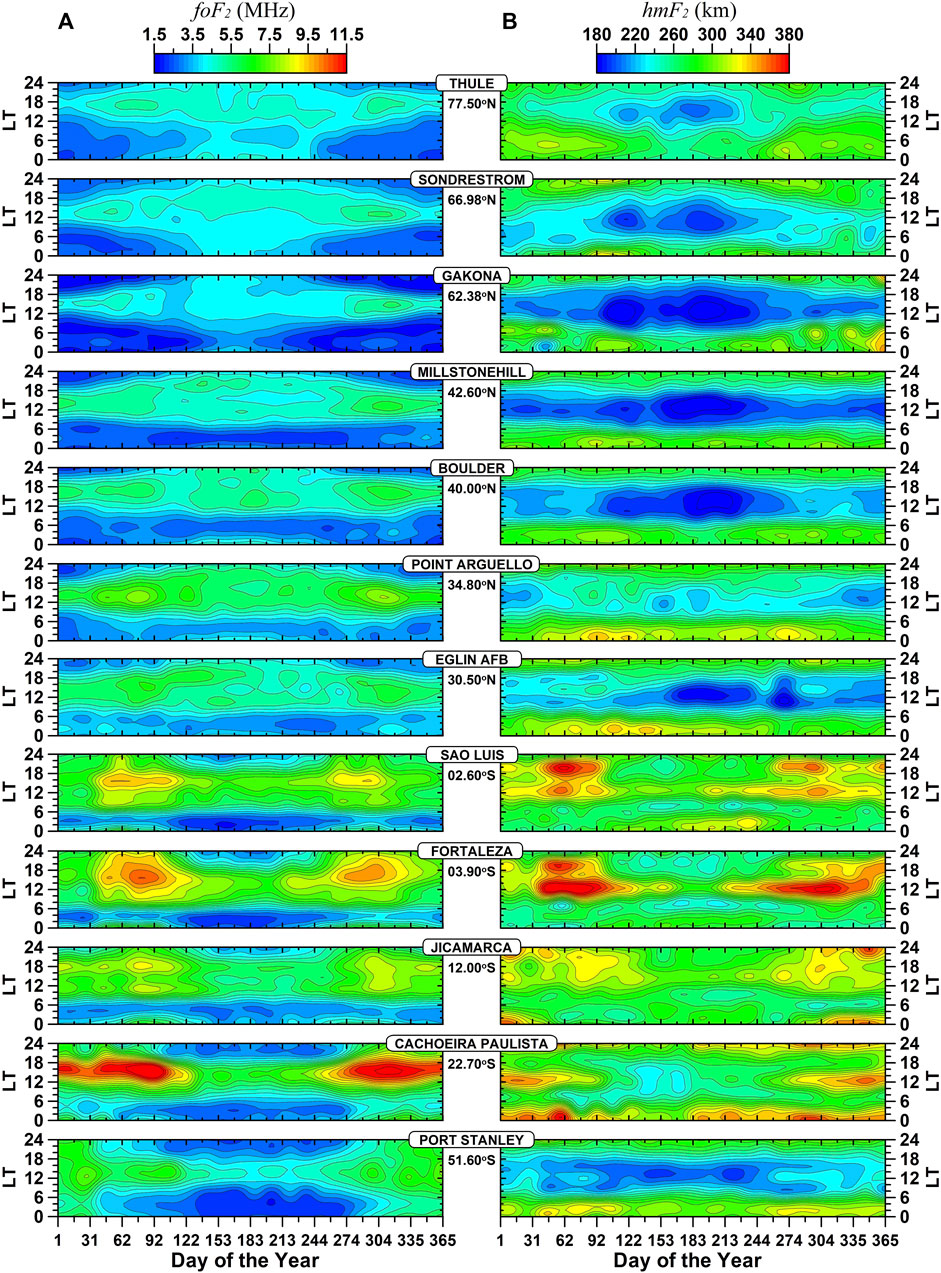
FIGURE 3. Contour plot of the hourly average of ionospheric peak parameters [foF₂ and hmF₂, (A,B), respectively] versus the day of the year sorted by the northern to the southern station (upper to bottom panels, respectively) composed from July 2007 to December 2010. Contour intervals are 0.5 MHz and 10 km for foF₂ and hmF₂, respectively.

Concerning foF₂ variability, Figure 3 also showed that, as expected, the higher values of electron density/critical frequency occurred during daytime (12–18 LT) for all stations analyzed, with two peaks centered on the equinoxes, except for CPL, which presented a maximum of foF₂ extending to the summer solstice. Similarly, to what was observed in hmF₂, the foF₂ over JIC was less intense than SAO. The higher values of these parameters over SAO may be associated with geomagnetic equator displacement from this region, making it, in this way, more susceptible to the effects generated by the winds. The large declination angle over SAO also can be relevant in this context.

3.2 Latitudinal variation of atmospheric solar tides modes present in hmF₂ and foF₂

In order to study the atmospheric tide components of the American sector, spectral analyses were applied to each of the seasonal climatologies of the stations shown in Figure 3 (an average of the hourly local time and day of the year from July 2007 to December 2010), for the two components of the F₂ peak. For such, considering the same methodology used by Santos et al. (2023), the Fast Fourier Transform was applied to the Digisonde data according to the following equation:

where ${xV}_{\left(t\right)}$ is the daily reconstructed variable of hmF₂ or foF₂ as a function of time in LT (t), $f_1$ is the fundamental frequency of the parameter to be reconstructed (1/24), $A0$ is the daily average of such parameter for a given day of the year, and finally, ${Am}_{\left(m\right)}$ and ${Bm}_{\left(m\right)}$ are the mth Fourier coefficients also as a function of time (LT). The terms ${Am}_{\left(m\right)}$ and ${Bm}_{\left(m\right)}$ together are the amplitudes for the harmonics m = 1 (24 h), m = 2 (12 h), and m = 3 (08 h). In this study, the spectral analysis was performed for the average of each day of the year for the period in the study. Figure 4, for example, considers the annual mean of tidal components and the amplitude for all the stations studied. Figures 5, 6, 8 on the other hand, present the daily variability of such components in terms of foF2 and hmF2 residual values (Δ), which in this case was calculated considering the tidal components of each day minus the annual mean values of Figure 4. For more details about the methodology used to extract and reconstruct the foF2 and hmF2 parameters based on the tidal components, see Brum et al. (2011). This same methodology also was used by Terra et al. (2020) to study the geomagnetic and solar dependency of MSTIDs highlighting its effectiveness in studies involving different phenomena of the ionosphere.

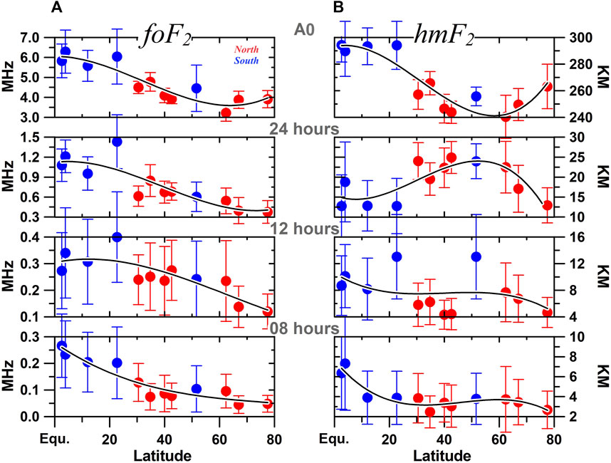
FIGURE 4. The annual average of the American Sector ionospheric peak amplitudes of the mean and the solar tide components as a function of latitude (red and blue represent the northern and southern hemispheres, respectively, while the continuous black lines are the best third-order polynomial approximation). The (A,B) are the results for foF₂ and hmF₂, respectively.

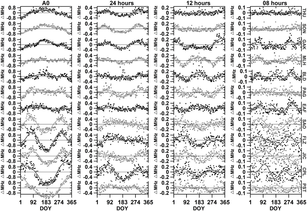
FIGURE 5. Daily variability of the amplitude (A0), diurnal (24 h), semidiurnal (12 h), and terdiurnal components (08 h) (from left to right) of the foF₂ parameter residuals for the twelve studied sites.

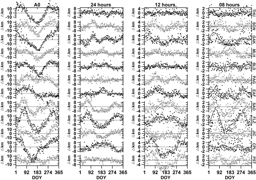
FIGURE 6. Same as Figure 5 but for the hmF₂ parameter.

Figure 4 shows the annual average of the American Sector ionospheric peak amplitudes of the mean and the solar tide components as a function of latitude. It is used red color to represent northern and blue to southern hemispheres. Although the distribution is not symmetrical and most part of the stations are located at the northern (see, for example, Figure 2), Figure 4 reveals that the annual average of all mean and harmonic components over the foF₂ and hmF₂ seem to be strongly dependent on latitude. In general, the mean and tidal modes are higher for the regions near the equator, except for hmF₂ diurnal tide, which is more intense at latitudes farther around 50^o from the equator. However, for this same mode, there is a decrease in the intensity of hmF₂ for latitudes higher than 60^o, which is the opposite of what is observed in the mean of the peak height parameter. According to Figure 4 (except the A0 component), the contribution of the diurnal tide (followed by semidiurnal and terdiurnal) was more relevant to determining the latitudinal variability in both F-layer peak parameters studied here.

Figure 5 shows, from the left to the right column of panels, the daily mean amplitude (A0), diurnal (m = 1, 24 h), semidiurnal (m = 2, 12 h), and terdiurnal (m = 3, 8 h) components for the foF₂ in respect of the day of the year (DOY) for all the stations described in Table 1 (Note that in this graph we are calling each contribution of the tidal and mean component as Δ, which is, from Eq. 1, for example, ΔA0, the first column on the left of Figure 5, would be just the average amplitude of the signal for a specific day without the contributions of annual amplitude value from Figure 4). The continuous lines represent the best FFT approximation to the data. It can be noted that the amplitude of foF₂ (A0, first block of panels of left) for the stations located more to the northern (THU, SON, and GAK) presented an annual component with a maximum occurring around the summer solstice. However, as it approaches the geomagnetic equator, there is observed not only an increase in the amplitude of this parameter but also a semiannual behavior, with a maximum around the equinoxes. It is interesting to note the return of an annual behavior for the stations located more southern (CPL and PST), similar to what was observed in stations located in the northern hemisphere. Regarding the diurnal, semidiurnal, and terdiurnal components, Figure 5 shows that these tidal modes presented an annual and semiannual component for all of the regions studied. For the case of the terdiurnal tide, it can be observed a terannual component both in the north and the south latitudes (MHL, BLD, EAF, JIC, CPL, and PST). Additionally, noting the low variability of semidiurnal and terdiurnal tides over THU and SON is interesting. It is also noteworthy the large amplitude of foF₂, as well as, the large variability of all tide’s modes over the low latitude station of CPL.

According to the panels shown in Figure 6, the amplitude of hmF₂ in most cases presented an annual and a semiannual component. Similar to what was observed in foF₂, the variability in the amplitude and different tidal modes of hmF₂ are higher over the sectors located in the southern. In this case, highlights the higher variability of semidiurnal tide for CPL and PST and terdiurnal tide for SAO and FLZ. For the hmF₂, it was also observed in the 8 h tide as a terannual component in some northern and southern localities, such as BLD, EAF, JIC, and CPL.

Figure 7 shows the FFT reconstruction of the amplitudes and tidal modes of foF₂ (Figure 7A) and hmF₂ (Figure 7B) in function of the geographic latitude (from 75°N to 45°S) and day of the year. The horizontal white lines between 45°N and 45°S represent the latitude range in which we have good data coverage, as indicated by the distribution of the studied stations in Figure 1. It can be noted that the amplitude of foF₂ over this range presents a dominant semiannual behavior, with two maxima around equinoxes (extending to the summer in the south hemisphere) and a deep minimum in the months of winter/summer in south/north latitudes, and a smaller minimum 6 months displaced. For the amplitude of hmF2, the annual cycle dominates with a deep minimum in June/July (mainly for latitudes higher than 45°N) and a flat maximum extending from October to April. Besides that, it can be noted that the amplitudes of both parameters are higher in the southern latitudes. The diurnal, semidiurnal, and terdiurnal components of foF₂ (Figure 7A) also present a semiannual behavior, with maximums being observed during the equinoxes. Distinct characteristics can be seen in the diurnal component of hmF₂, which showed four peaks along the year for all latitudes, but with the higher contribution being observed in the north hemisphere. An annual behavior is seen in semidiurnal mode, with a maximum around the summer in the south latitudes. The opposite was observed in north latitudes until 45°. For the latitudes higher than this, similar behavior is seen when compared to south latitudes. Finally, the terdiurnal tide presented three maximums centered in the equator/southernmost for hmF₂/foF₂.

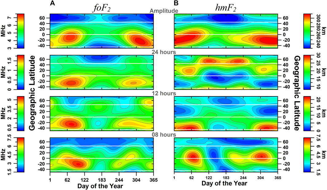
FIGURE 7. Contour plots of the seasonal climatology of the amplitude of the atmospheric tides’ components of foF₂ and hmF₂ [(A,B), respectively] as a function of day of the year and geographic latitude for the deep solar minimum.

To better visualize the impacts of atmospheric tides in the foF2 and hmF2 parameters, Figure 8 was constructed, disregarding the annual variability average similar to what was presented in Figures 5, 6. In a general way, it can be observed that the foF2 mean amplitude presented a predominant annual component, with a peak around summer, extending to March equinoxes, and a minimum in the winter in the south hemisphere. The 24 h component presents a semiannual behavior with maximums around equinoxes and a minimum during the winter/summer in the south/north. In this case, the contribution of diurnal tide is more pronounced in south latitudes, except at the end of the year, when the intensity of diurnal tide is higher for high latitudes. The diurnal tide is lower for regions between the equator and 45°N and does not present a considerable variation throughout the year. The 12 h mode showed more/less substantial contributions in winter/equinoxes in north latitudes. Between the equator and south latitudes, a maximum can be observed in March equinoxes and a minimum around the winter. Regarding the terdiurnal tide, relevant contributions can be noted both in the equator and north and south latitudes. Over the equator, the maximums were observed around DOY 62 and DOY 304, and the minimum between May and June.

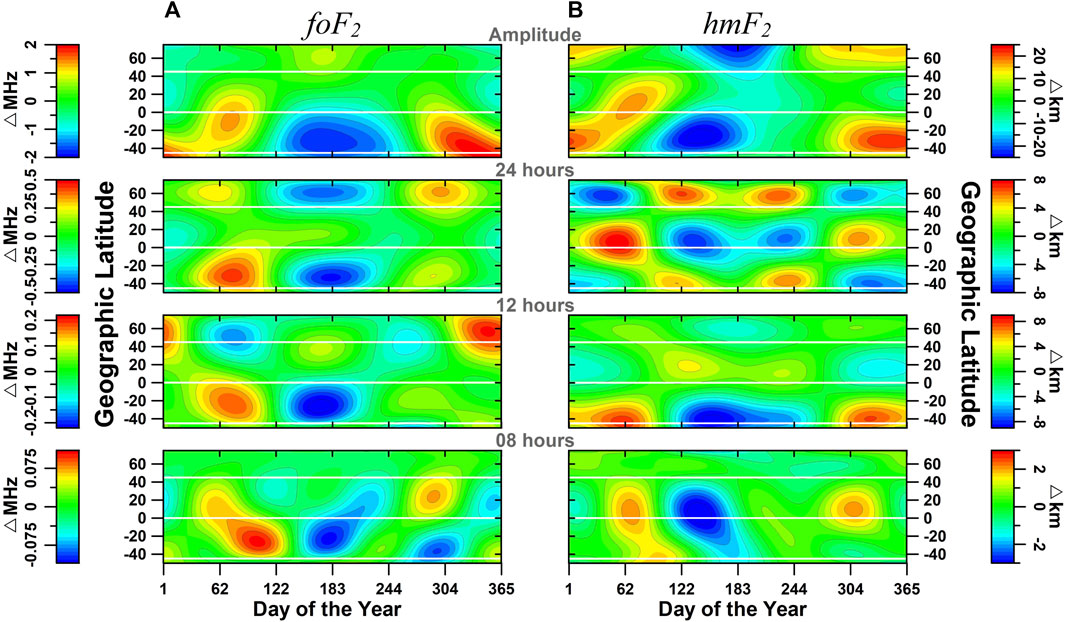
FIGURE 8. Contour plots of the residual annual variation of the amplitude e atmospheric tides components of foF² and hmF² [(A,B) respectivitely] in function of day of the year and geographic latitude during the deep solar minimum.

The results for hmF2 (Figure 8B) show that the amplitude of hmF2 is higher in the summer/winter in the south/north hemisphere and lower in the winter/summer in the north/south hemisphere. It is interesting to note the high amplitudes in the March equinox for the regions between the equator and 45°N. For the diurnal component of hmF2, the higher variability can be seen in the north hemisphere, with four peaks for latitudes higher than 45°N, and two around the equinoxes between the equator and 45°N. Regarding the semidiurnal component highlights the strong/weak contribution to hmF2 in summer/winter over the south hemisphere. For latitudes from the equator until 45°N, a slight intensification can be observed around the DOY 122 and 244, and a minor contribution during the winter. Finally, the 8 h mode presented a peak around the March equinox (extending to DOY 122) in the south latitudes and another in the September equinox centered in the equator. A minimum is observed between DOY 122–183, extending from 30°N to 45°S.

4 Discussion

The purpose of this paper is to investigate the impacts of solar atmospheric tides (diurnal, semidiurnal, and terdiurnal modes) and the amplitude on the variability of the parameters of critical frequency (foF₂) and peak height (hmF₂) of the F₂-layer in the American sector during the transition of solar cycles #23 and #24. According to some authors, this period presented an unusual behavior, being more profound, longer, and also geomagnetically quieter when compared to the previous minima. These conditions are very appropriate for understanding the foF₂ and hmF₂ variability since, in this case, the contamination of geomagnetic activity in these data can be minimized. In this context, this work is developed.

The foF2 and hmF2 are considered the two essential parameters of the F2-region for ionospheric radio wave propagation studies, as well as for understanding the physics of this region. The results presented here revealed interesting characteristics and it will be discussed in this section. Figure 3 reveals clearly that the higher intensities of height and frequency were observed in the stations near the equator and the south latitudes. In part, this behavior can be related to the lack of stations near to magnetic equator on the north side. As shown in the map of Figure 1, although the latitudinal distribution of Digisonde is uneven and most concentrated on the north side (7 of 12 stations), they are located more distant from the equator when compared to the southern stations. However, the analysis made in Figures 7, 8, which consider the reconstruction of the signal using FFT, indicates convincing evidence that, in general, the atmospheric tides seem to be more intense over the equator and in the South American sector, especially over Brazilian region (except in some cases).

Figure 5 shows that the amplitude of foF2 generally presents a clear annual and semiannual behavior. The annual component was observed for the stations located more to the northern/southern, with a maximum occurring around the summer/winter solstice. However, a transition to semiannual behavior was noted for stations closest to the geomagnetic equator, with a maximum occurring around the equinoxes. Zhu et al. (2023) recently reported this same feature. Based on the observations from the Langmuir probe (LAP) onboard the China Seismo-Electromagnetic Satellite (CSES) at an altitude of 500 km during the period between May 2018 and April 2022, Zhu et al. (2023) noted that the electron density dominant period is characterized by a transition of an annual to semiannual variation from middle to low and equatorial latitudes. Burns et al. (2012) also showed that the semiannual variation dominated the low-latitude NmF2 while annual variation dominated at high latitudes (75°Mlat). Based on COSMIC IRO observations, Zeng et al. (2008), in turn, showed that the F2-layer density presented an annual asymmetry in which the December NmF2 is, on a global average, more significant than the June NmF2 in both hemispheres. Although our ground-based observations do not present particularly good latitudinal coverage, our results agree with previous works.

The average annual amplitude of hmF₂ and foF₂ in Figure 4 showed that the different tidal modes were more intense for the regions located near the equator, except for the case of 24 h tide of hmF₂, that in this case, was more significant for latitudes higher than 45°N. It also can be noted that the semidiurnal and terdiurnal tides, on average, contributed similarly to the variability of hmF₂ for all latitudes studied. On the other hand, for foF₂, the different components of tides were more important to regions near the equator. The individual analyses for each station (see Figure 5), in turn, evidenced that the higher oscillation of tides occurred in the southern latitudes. For example, in the Brazilian low latitude regions of CPL and FLZ, more considerable variability can be seen in the amplitude A0, 24 h, 12 h, and 8 h modes both in the foF₂ and hmF₂ data. Figure 5 also shows interesting results about the conjugated points of PST and EAF. In this case, the A0 of foF₂ of the station located to the south (PST) is higher than those located to the north (EAF). However, comparable results were found in tidal components over these sectors. On the other hand, the results of hmF₂ show the different contributions of semidiurnal mode for these regions, this mode being more relevant in the south hemisphere.

Banks and Kockarts (1973) mentioned that competition between chemical and transport processes controls the ionosphere’s density profiles. At altitudes above 150–200 km, the ion composition and concentration are no longer determined by local effects but also by a more complicated coupling involving the diffusion of the ions via geomagnetic field lines, winds, and electric fields (Rishbeth and Garriott, 1969). Figure 3, for example, shows that the equatorial and lower latitudes ionosphere (especially those in the South Hemisphere) present a peculiar behavior compared to the ionosphere at higher latitudes. At the equatorial region of JIC, for example, hmF₂ reached higher intensities after 12 LT in the equinoxes and summer months. An intensification around 18 LT also was seen and probably is related to the development of prereversal enhancement of the zonal electric field at sunset times (Farley et al., 1986; Kelley et al., 2009). Comparing the results from JIC with SAO, which are regions located a little below the geomagnetic equator, it can be observed that over SAO, an intensification of F-layer peak height around 12 LT for the whole year (with lower/higher intensity during the winter/equinoxes—summer months) was seen, as well as the PRE development, that in this case was more intense around in the March equinoxes when compared to September equinoxes and summer. It is believed that the differences observed between JIC and SAO can be directly related to the large declination angle to which the Brazilian region is subject (Abdu et al., 1981) and also the geomagnetic equator displacement from SAO. For the regions more distant from the equator, the magnetic field configurations make the effect of the electromagnetic vertical drift lower. As the equator moves away from a given region, the F layer is susceptible to the impacts generated by the equatorward neutral air wind that can contribute to elevating the layer to higher altitudes. Then, the more intense values in hmF₂ of SAO can be associated with the additional effects generated by the winds. Additionally, it is important to mention that the low values of hmF₂ observed here can be directly associated with the weaker electric field observed during this period of extreme minimum solar activity. Comparing results from SAO and FLZ, we observed that the PRE also was present clearly in March equinoxes over SAO.

Concerning the increase in hmF₂ at 12 LT, it is observed that this feature was remarkably more intense over FLZ. Over the low latitude region of CPL, a similar intensification of the hmF₂ (less intensity) was observed around 12 LT (with a peak centered in December and January) and after 23 LT. Although FLZ is not considered an equatorial station, it is nearer to the equator than CPL. Then, electric fields would also influence the layer height of this region, justifying the higher intensities of hmF2 over this sector when compared to CPL. The intensification of hmF2 near midday can be associated with EIA development. Over CPL and PST, the PRE occurrence was absent. Still, about the hmF2, the low values of this parameter during the daytime over the stations located in the north hemisphere during the summer can be noted. The reasons to explain this can be related to chemical and dynamical processes. More investigations need to be done to understand better these phenomena.

Regarding foF₂, Figure 3A show the occurrence of peak around the daytime during equinoxes, extending to summer/winter months in some cases, being more intense in regions near to equator and south latitudes. The higher values around the equinoxes are related to the fact that during this season, the sun shines directly over the equatorial region and thus leads to the strongest ionization over these regions. Highlights the increase of foF2 starting at sunrise hours, attaining a maximum of around 12–14 LT in almost all stations studied. The rapid rise in ionization from its nighttime minimum occurs due to photoionization. The ionization in the F-region below about 300 km is under strong solar control, peaking at noon when the solar zenith angle is smallest and then decreasing symmetrically as this angle increases (Banks and Kockarts, 1973). Another interesting characteristic observed in foF₂ distribution is the weakening of the equatorial ionization anomaly. Batista and Abdu (2004) mentioned the eastward electric field during the day produces an upward drift at and close to the magnetic equator, which is responsible for initiating the well-known fountain effect. This upward drift elevates the plasma of the equatorial region to high altitudes. However, due to the gravity effects and plasma pressure gradients, this plasma diffuses along the magnetic field lines resulting in a depletion of F-region plasma density at the magnetic equator and two crests of plasma density on either side of the magnetic equator (about ±15–20° dip latitude). To this phenomenon, it was given the name of EIA. At sunset, when the E layer conductivity drastically decay, this eastward electric field suffer an intensification before reversing westward, which is known as PRE. This causes a substantial decrease of foF₂ in the equator and an increase of ionization in low latitudes, a few hours after PRE in the equator. However, our results show low plasma intensity during the nighttime over CPL, a region located in a crest of anomaly. This feature reflects the low intensity of zonal electric field/vertical plasma drift during the period of solar minimum condition.

5 Conclusion

In this work, we have investigated the climatology of atmospheric solar tidal mode effects on hmF2 and foF2 over the American sector during solar minimum between cycles #23 and #24. In summary, the main findings of this work are:

• The hmF2 and foF2 strongly depend on latitude and seasonality, being more intense in the stations located south of the geomagnetic equator.

• The mean amplitudes of foF₂ and hmF₂ and the different components of tides are strongly dependent on latitude.

• In general, the mean amplitude and tidal modes are higher for the regions near the equator, except for hmF₂ diurnal tide, which is more intense at latitudes further distant from the equator.

• The seasonal variability of the amplitude of hmF₂ and foF₂ in most of the cases presented an annual and semiannual variation. Likewise, what was observed in foF₂, the variability in the mean amplitude and different modes of tides of hmF₂ are higher over the sectors located in the southern hemisphere.

• The terannual behavior was observed over the 8 h tide in both hmF2 and foF2, and also in diurnal tide observed in hmF2 of some localities in the northern and southern hemispheres.

• The differences observed in the hmF₂ and foF₂ of the regions of JIC and SAO can be associated with the large magnetic declination angle of the Brazilian station and also due to the geomagnetic equator displacement of SAO. This last condition makes the effect of meridional wind in the vertical movement of the ionosphere over this sector relevant compared to an equatorial site.

• The low value of hmF₂ over the northern latitudes during the summer can be associated with a lower concentration of neutral oxygen during this period.

Data availability statement

The Digisonde data used in this work can be found in the GIRO data center (https://giro.uml.edu/didbase/scaled.php).

Author contributions

AS: Investigation, Writing–original draft, Writing–review and editing. GY: Supervision, Writing–review and editing. AP: Supervision, Writing–review and editing. CB: Investigation, Methodology, Writing–review and editing. IB: Writing–review and editing. JHS: Writing–review and editing. VA: Writing–review and editing. PB: Writing–review and editing. MA: Writing–review and editing. JRS: Writing–review and editing. PM: Writing–review and editing. CW: Funding acquisition, Writing–review and editing. HL: Writing–review and editing. ZL: Project administration, Writing–review and editing.

Funding

The authors declare financial support was received for the research, authorship, and/or publication of this article. This research was supported by the International Partnership Program of Chinese Academy of Sciences (grants 183311KYSB20200003 and 183311KYSB20200017). JS thanks the CNPq (grant 311840/2022-1) and the Instituto Nacional de Ciência e Tecnologia GNSS-NavAer supported by CNPq (465648/2014-2), FAPESP (2017/50115-0) and CAPES (88887.137186/2017-00).

Acknowledgments

AS and VA would like to thank the China-Brazil Joint Laboratory for Space Weather (CBJLSW), the National Space Science Center (NSSC), Chinese Academy of Sciences (CAS) for supporting their postdoctoral research. CB would like to thank the support from NSF Award AGS-2221770. The Digisonde data was obtained in the GIRO data center (https://giro.uml.edu/didbase/scaled.php). The Kp index was obtained from the World Data Center for Geomagnetism, Kyoto (http://wdc.kugi.kyoto-u.ac.jp/index.html, accessed on 15 March 2023), and the Solar Radio Flux (F10.7 cm) from the Natural Resources Canada, Solar radio flux-archive of measurements website (http://www.spaceweather.gc.ca/solarflux/sx-5-en.php, accessed on 15 March 2023).

Conflict of interest

The authors declare that the research was conducted in the absence of any commercial or financial relationships that could be construed as a potential conflict of interest.

Publisher’s note

All claims expressed in this article are solely those of the authors and do not necessarily represent those of their affiliated organizations, or those of the publisher, the editors and the reviewers. Any product that may be evaluated in this article, or claim that may be made by its manufacturer, is not guaranteed or endorsed by the publisher.

References

Abdu, M. A., Bittencourt, J. A., and Batista, I. S. (1981). Magnetic declination control of the equatorial F region dynamo electric field development and spread F. J. Geophys. Res. Space Phys. 86 (A13), 11443–11446. doi:10.1029/JA086iA13p11443
Andrioli, V. F., Xu, J., Batista, P. P., Resende, L. C. A., Da Silva, L. A., Marchezi, J. P., et al. (2022). New findings relating tidal variability and solar activity in the low latitude MLT region. J. Geophys. Res. Space Phys. 127, e2021JA030239. doi:10.1029/2021JA030239
Batista, I. S., and Abdu, M. (2004). Ionospheric variability at Brazilian low and equatorial latitudes: comparison between observations and IRI model. Adv. Space Res. 34 (9), 1894–1900. doi:10.1016/j.asr.2004.04.012
Brum, C. G. M., Rodrigues, F. S., dos Santos, P. T., Matta, A. C., Aponte, N., Gonzalez, S. A., et al. (2011). A modeling study of foF2 and hmF2 parameters measured by the Arecibo incoherent scatter radar and comparison with IRI model predictions for solar cycles 21, 22, and 23. J. Geophys. Res. 116, A03324. doi:10.1029/2010JA015727
Burns, A. G., Solomon, S. C., Wang, W., Qian, L., Zhang, Y., and Paxton, L. J. (2012). Daytime climatology of ionospheric NmF2 and hmF2 from COSMIC data. J. Geophys. Res. 117, A09315. doi:10.1029/2012JA017529
Cai, X., Burns, A. G., Wang, W., Qian, L., Pedatella, N., Coster, A., et al. (2021). Variations in thermosphere composition and ionosphere total electron content under “geomagnetically quiet” conditions at solar-minimum. Geophys. Res. Lett. 48, e2021GL093300. doi:10.1029/2021GL093300
Davis, R. N., Du, J., Smith, A. K., Ward, W. E., and Mitchell, N. J. (2013). The diurnal and semidiurnal tides over Ascension Island (° S, 14° W) and their interaction with the stratospheric quasi-biennial oscillation: studies with meteor radar, eCMAM and WACCM, Atmos. Chem. Phys. 13, 9543–9564. doi:10.5194/acp-13-9543-2013
Farley, D. T., Bonelli, E., Fejer, B. G., and Larsen, M. F. (1986). The prereversal enhancement of the zonal electric field in the equatorial ionosphere. J. Geophys. Res. Space Phys. 91 (A12), 13723–13728. doi:10.1029/JA091iA12p13723
Fontes, P. A., Muella, M. T. D. A. H., Resende, L. C. A., Andrioli, V. F., Fagundes, P. R., Pillat, V. G., et al. (2022). Effects of the terdiurnal tide on the sporadic E (Es) layer development at low latitudes over the Brazilian sector. Ann. Geophys. 41, 209–224. doi:10.5194/angeo-41-209-2023
Forbes, J. M. (1996). Planetary waves in the thermosphere-ionosphere system. J. Geomag. Geoelec 48, 91–98. doi:10.5636/jgg.48.91
Forbes, J. M. (2021). Atmosphere-ionosphere (A-I) coupling by solar and lunar tides, 157–181. doi:10.1002/9781119815631.ch9
Forbes, J. M., Palo, S. E., and Zhang, X. (2000). Variability of the ionosphere. J. Atmos. Solar-Terrestrial Phys. 62 (8), 685–693. ISSN 1364-6826. doi:10.1016/S1364-6826(00)00029-8
Griffith, M. J., and Mitchell, N. J. (2022). Analysis of migrating and non-migrating tides of the Extended Unified Model in the mesosphere and lower thermosphere. Ann. Geophys. 40, 327–358. doi:10.5194/angeo-40-327-2022
Hagan, M. E., and Forbes, J. M. (2002). Migrating and nonmigrating diurnal tides in the middle and upper atmosphere excited by tropospheric latent heat release. J. Geophys. Res. Atmos. 107. ACL 6-1–ACL 6-15. doi:10.1029/2001JD001236
Kelley, M. C., Ilma, R. R., and Crowley, G. (2009). On the origin of pre-reversal enhancement of the zonal equatorial electric field. Ann. Geophys. 27, 2053–2056. doi:10.5194/angeo-27-2053-2009
Lindzen, R. S., and Chapman, S. (1969). Atmospheric tides. Space Sci. Rev. 10, 3–188. doi:10.1007/bf00171584
Manson, A. H., Meek, C. E., Teitelbaum, H., Vial, F., Schminder, R., Kürschner, D., et al. (1989). Climatologies of semi-diurnal and diurnal tides in the middle atmosphere (70–110 km) at middle latitudes (40–55°). J. Atmos. Terr. Phys. 51, 579–593. doi:10.1016/0021-9169(89)90056-1
Mathews, J. D., Morton, Y. T., and Zhou, Q. (1993). Observations of ion layer motions during the AIDA campaign. J. Atmos. Terr. Phys. 55 (3), 447–457. doi:10.1016/0021-9169(93)90080-i
Mendillo, M., Rishbeth, H., Roble, R., Damboise, E., and Wroton, J. (1998). Indian nuclear tests prompt worldwide concern. EOS, Trans. 79 (17), 238. doi:10.1029/98eo00175
Millward, G. H., Müller-Wodarg, I. C. F., Aylward, A. D., Fuller-Rowell, T. J., Richmond, A. D., and Moffett, R. J. (2001). An investigation into the influence of tidal forcing on F region equatorial vertical ion drift using a global ionosphere-thermosphere model with coupled electrodynamics. J. Geophys. Res. Space Phys. 106 (A11), 24733–24744. doi:10.1029/2000JA000342
Oikonomou, C., Haralambous, H., Leontiou, T., Tsagouri, I., Buresova, D., and Mošna, Z. (2021). Intermediate descending layer and Sporadic E tidelike variability observed over three mid-latitude ionospheric stations. Adv. Space Res. 69, 96–110. doi:10.1016/j.asr.2021.08.038
Rishbeth, H., and Garriott, O. K. (1969). IV. Transport processes in the ionosphere. Int. Geophys. 14, 126–159. doi:10.1016/S0074-6142(09)60024-3
Sagawa, E., Immel, T. J., Frey, U., and Mende, S. B. (2005). Longitudinal structure of the equatorial anomaly in the nighttime ionosphere observed by IMAGE/FUV. J. Geophys. Res. 110, A11302. doi:10.1029/2004JA010848
Sakazaki, T., Fujiwara, M., and Shiotani, M. (2018). Representation of solar tides in the stratosphere and lower mesosphere in state-of-the-art reanalyses and in satellite observations. Atmos. Chem. Phys. 18, 1437–1456. doi:10.5194/acp-18-1437-2018
Santos, Â. M., Brum, C. G. M., Batista, I. S., Sobral, J. H. A., Abdu, M. A., Souza, J. R., et al. (2023). Ionospheric variability over the Brazilian equatorial region during the minima solar cycles 1996 and 2009: comparison between observational data and the IRI model. Atmosphere 14, 87. doi:10.3390/atmos14010087
Terra, P., Vargas, F., Brum, C. G. M., and Miller, E. S. (2020). Geomagnetic and solar dependency of MSTIDs occurrence rate: a climatology based on airglow observations from the arecibo observatory rof. J. Geophys. Res. Space Phys. 125 (7), e2019JA027770. doi:10.1029/2019JA027770
Yamazaki, Y., and Richmond, A. D. (2013). A theory of ionospheric response to upward-propagating tides: electrodynamic effects and tidal mixing effects. J. Geophys. Res. Space Phys. 118, 5891–5905. doi:10.1002/jgra.50487
Zeng, Z., Burns, A., Wang, W., Lei, J., Solomon, S., Syndergaard, S., et al. (2008). Ionospheric annual asymmetry observed by the COSMIC radio occultation measurements and simulated by the TIEGCM. J. Geophys. Res. 113, A07305. doi:10.1029/2007JA012897
Zhai, C., Cai, X., Wang, W., Coster, A., Qian, L., Solomon, S. C., et al. (2023). Mid-latitude ionospheric response to a weak geomagnetic activity event during solar minimum. J. Geophys. Res. Space Phys. 128, e2022JA030908. doi:10.1029/2022JA030908
Keywords: ionosphere, F-region peak, solar atmospheric tides, solar minimum, latitudinal dependence
Citation: Santos AM, Yang G, Pimenta AA, Brum CGM, Batista IS, Sobral JHA, Andrioli VF, Batista PP, Abdu MA, Souza JR, Manoharan PK, Wang C, Li H and Liu Z (2024) Climatology of atmospheric solar tidal mode effects on ionospheric F2 parameters over the American sector during solar minimum between cycles #23 and #24. Front. Astron. Space Sci. 11:1325218. doi: 10.3389/fspas.2024.1325218
Received: 20 October 2023; Accepted: 05 January 2024;
Published: 25 January 2024.
Edited by:
Amitava Guharay, Physical Research Laboratory, IndiaReviewed by:
Sardar Singh Rao, Udaipur Solar Observatory, IndiaXuguang Cai, University of Colorado Boulder, United States
Copyright © 2024 Santos, Yang, Pimenta, Brum, Batista, Sobral, Andrioli, Batista, Abdu, Souza, Manoharan, Wang, Li and Liu. This is an open-access article distributed under the terms of the Creative Commons Attribution License (CC BY). The use, distribution or reproduction in other forums is permitted, provided the original author(s) and the copyright owner(s) are credited and that the original publication in this journal is cited, in accordance with accepted academic practice. No use, distribution or reproduction is permitted which does not comply with these terms.
*Correspondence: A. M. Santos, angelamacsantos@gmail.com