EXOSpy: A python package to investigate the terrestrial exosphere and its FUV emission

1 Introduction

In 1972, the Apollo 16 mission retrieved the first wide-field far-ultraviolet (FUV) imagery of the earth and revealed the vast extent of the terrestrial exosphere, also known as the “geocorona” (Carruthers et al., 1976). This outermost atmospheric layer extends from several hundreds of kilometers above the earth’s surface (∼500 km) out to several tens of earth radii (∼ 60 R_E) (Baliukin et al., 2019). The most dominant component in this region is atomic hydrogen (H) that resonantly scatters FUV emission centered at the 121.56 nm wavelength (Ly-α). Furthermore, the exosphere is embedded within the many distinct plasma environments spanning the topside ionosphere, plasmasphere, ring-current system, and solar wind. Charge exchange interactions between exospheric H atoms and ambient ions are well known to play a crucial role in governing the earth’s transient response to space weather, both by dissipating magnetospheric ring current energy through the generation of energetic neutral atoms (ENAs) and by driving the ion transport responsible for plasmaspheric refilling after geomagnetic storms (Ilie et al., 2012; Krall et al., 2018; Cucho-Padin et al., 2020). Due to its relevance in magnetospheric physics, efforts have been made to estimate three-dimensional (3-D), time-dependent, and global H density distributions using sophisticated remote sensing techniques based on measurements of the terrestrial Ly-α emission (Bailey and Gruntman, 2011; Zoennchen et al., 2015; Cucho-Padin and Waldrop, 2018; 2019).

The planetary and astrophysics community also requires observations of Ly-α emission from extra-solar targets to understand stellar chromospheres and transition regions, model photo-chemistry in planetary/exoplanetary atmospheres, and measure the abundance of neutral hydrogen in the Inter-stellar medium (ISM) (Youngblood et al., 2016). However, such observations carried out from low-Earth orbits (LEO) and usually with optical spectrometers are significantly contaminated by the bright geocoronal emission, e.g., ∼ > 10 kR for a dayside limb observation at 600 km altitude (kR = kilo Rayleigh, 1 Rayleigh = 10⁶/4π photons/sec/str/cm²). Also, the terrestrial exosphere is dynamic, and its spatial density distribution responds to seasonal variations, solar cycles, and active geomagnetic conditions, ultimately resulting in variations of Ly-α radiance of ∼ > 500 R (Waldrop and Paxton, 2013; Cucho-Padin and Waldrop, 2019) that might be of similar magnitude to the emission from extra-terrestrial objects. These conditions motivate planetary scientists and astrophysicists to pursue sophisticated techniques to avoid and/or subtract the terrestrial Ly-α emission from their measurements. For example, Youngblood et al. (2016) conducted a stellar characterization study using observations from the Cosmic Origins Spectrograph (COS) onboard the Hubble Space Telescope (HST). To avoid geocoronal contamination, measurements were restricted to happen during the time of the year when the earth’s heliocentric velocity would allow the geocoronal Ly-α emission to coincide with the attenuated stellar Ly-α line core. In other words, due to a Doppler effect, the Ly-α line of the target is not located exactly at 121.56 nm but red- or blue-shifted depending on velocity direction. Then, the geocoronal emission line was directly subtracted using sky background measurements. Another technique includes fitting geocoronal measurements to a Gaussian function (Wood et al., 2005) or other airglow templates (Bourrier, V. et al., 2018) to estimate the line-integrated intensity and subtract it off from the measurements.

A similar approach used by Bhattacharyya et al. (2017) to characterize the spatial distribution of H in the Martian exosphere using the Advance Camera for Survey (ACS) instrument onboard HST, is to observe Mars when the geocoronal Ly-α is sufficiently doppler-shifted with respect to the Mars line. This ensures that the geocoronal contamination can be subtracted off from the total observed intensity without dealing with complicated radiative transfer effects. However, an additional HST orbit is required to measure the background emission intensity since ACS is a broad-band UV imager.

It is evident to the UV astronomy community in general that an accurate specification of the terrestrial exospheric Ly-α emission is of utmost importance not only to increase the frequency and precision of target observations under less-restrictive conditions but also to increase the efficiency of space-based asset utilization to allow for better characterization of the target properties with more accurate estimations of the background contamination. In this work, we have developed a python-based package EXOSpy that brings together state-of-the-art and publicly available H exospheric models to be accessible to the scientific community through a set of simple functions. Furthermore, EXOSpy enables the user to calculate exospheric emissions that serve (i) to validate exospheric models with actual Ly-α radiance data, (ii) to estimate exospheric contamination that may affect extra-terrestrial observations, and (iii) to support UV instrument design. In this manuscript, we outline EXOSpy’s architecture and highlight its key capabilities. In Section 2, we describe the main features of this package, such as the exospheric models included in it and the core operations to estimate Ly-α radiance. In Section 3, we show practical applications of EXOSpy. Finally, in Section 4 we summarize the conclusions of this project and present future directions to improve this package.

2 Description of the EXOSpy python-based package

EXOSpy is an open-source python package that allows the user to explore several H exospheric models and generate column-integrated Ly-α intensities for single-pixel photometers or wide field-of-view (FOV) imagers that could potentially facilitate mission design efforts as well as aid the removal of exospheric background emission.

2.1 Terrestrial exospheric models

EXOSpy includes physics- and data-based exospheric models described in this section. We refer the reader to the cited references below as well as the EXOSpy’s website https://exospy.readthedocs.io/for further details.

Chamberlain (1963) developed a physics-based exospheric model to determine density distribution of species at altitudes where collisions between them can be neglected. Here, H atoms are assumed to be thermalized through neutral-neutral collisions at the boundary of the collisional and collisionless atmosphere, termed as the exobase ($\sim 500$ km altitude), and then adopt ballistic or escaping trajectories to space. The H density distribution model is reported as an analytical altitude-dependent function that only requires values of H density (n_exo) and neutral temperature (T_exo) at the exobase, both of which can be specified by external models, such as the well-known model NRLMSIS2.0 (Emmert et al., 2021).

Bailey and Gruntman (2011) developed an exospheric model based on parametric fitting to a spherical harmonic function using single-day measurements of scattered Ly-α emission acquired by the Lyman-Alpha Detector (LAD) onboard the Two-Wide angle Imaging Neutral-atom Spectrometers (TWINS) mission. The approach used in this study leverages the linearity between the H density and its emission that occurs when the medium is optically thin, i.e., the density is low enough such that each H atom scatters a solar Ly-α photon only once. At earth, the exospheric optically thin region is located beyond 3 R_E geocentric distance. In addition, the TWINS/LAD apogee of ∼ 7.2 R_E and its nadir viewing geometry allows only partial observation of the exosphere, i.e., a single LAD line-of-sight (LOS) acquires emission starting from a radial position $\sim 7.2R_E$ towards infinity on the opposite side, but it cannot observe emission behind the instrument where there is still significant exospheric density with approximate values of 10 ∼ 100 cm⁻³ (Cucho-Padin et al., 2022b). Thus, exospheric density reconstructions using TWINS/LAD Ly-α data typically set 8R_E as an upper boundary since the estimation of the region behind the sensor may feature high uncertainty. Hence, retrieved 3-D, global H density distributions for this model are only valid from the 3 to 8 R_E region. Zoennchen et al. (2015) used a similar approach using multi-day data acquired by LAD/TWINS to generate a model for solar minimum conditions (with data acquired in 2008 and 2010) and solar maximum conditions (with data acquired in 2012). The region of validity for these two models is also restricted to a region from 3 to 8 R_E. Furthermore, Zoennchen et al. (2022) estimated an H density radial profile using Ly-α measurements from the Ultraviolet Imaging Spectrograph (UVIS) onboard the CASSINI spacecraft during an earth flyby on 18 August 1999, on its way to Saturn (Esposito et al., 2004; Werner et al., 2004). These radiance data were fitted to a spherical function to yield an exospheric profile valid from 3 to 15 R_E. Recently, Cucho-Padin et al. (2022b) derived a 3-D model of the outer exosphere using a single global image acquired by the Lyman-Alpha Imager CAmera (LAICA) onboard the Proximate Object Close Flyby with Optical Navigation (PROCYON) spacecraft when it was located at ∼2000 R_E from earth. The H density model is reported as spherical harmonics coefficients with a valid region that ranges from 6 to 15 R_E.

Estimation of neutral densities is also possible through remote sensing of soft X-ray emissions, which are generated by the charge exchange interaction between heavy charged solar wind particles (e.g., O⁺⁷ and O⁺⁸) and exospheric neutral atoms. Connor and Carter (2019) estimate H density in the vicinity of the terrestrial magnetosheath, i.e., the subsolar point at ∼10 R_E, using simultaneous measurements of soft X-ray radiance acquired by the XMM-Newton mission and in situ ion density, acquired by Cluster and Geotail missions. The H density for two events during solar maximum conditions (October 2001 and May 2003) are reported as a spherical function. Following a similar methodology, Jung et al. (2022) used XMM-Newton radiance data and THEMIS ion density data to determine an H density profile during solar minimum conditions (November 2008) and it is also reported as a spherical function. Since both studies utilized data from magnetosheath (located within the optically thin exospheric region), we consider the valid region of their models to range from 3 R_E to ∼12 R_E, where the bow shock (the outer boundary of magnetosheath) is typically located (Fairfield, 1971). Table 1 provides a summary of data-based models included in this package.

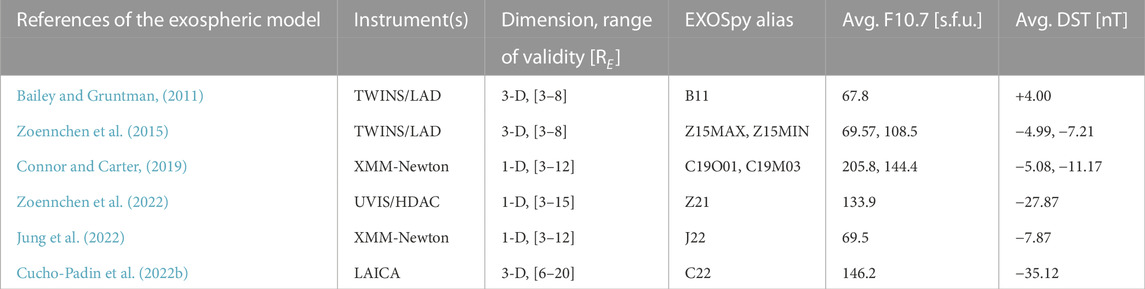
TABLE 1. Data-based exospheric models included in the EXOSpy package. Solar radio flux at 10.7 cm (F10.7) and the geomagnetic disturbance index (DST) provide additional information regarding solar and geomagnetic conditions during the Ly-α data acquisition, which was used to generate the model. Values of F10.7 and DST are expressed as a day or multi-day averages. The reader is referred to the references for further details. DST values were obtained from the World Data Center for Geomagnetism, Kyoto. F10.7 values were obtained from the LASP Interactive Solar Irradiance Data Center, Colorado, United States.

EXOSpy provides the user with functions to generate and visualize H density distributions. For example, the function draw1DHmodel receives a 1-D model alias (see Table 1) and an altitude range (in units of R_E) as inputs to produce the corresponding H density profile, as a numpy array, as well as a density vs altitude graph. Similarly, the function draw3DHmodel generates a 3-D H density profile and plots for the meridional and equatorial planes and spherical shell for a given geocentric radius. In Figure 1, panels (A) (B) and (C) show plots for the 3-D H density distribution model derived by Zoennchen et al. (2015) for solar maximum conditions (EXOSpy’s alias Z15MAX). Specifically, panel (A) shows the equatorial plane, panel (B) shows a meridional (pole-to-pole) plane containing the subsolar point, and panel (C) shows a spherical shell at a geocentric radius of 5 R_E. In addition, panel (D) shows a comparison between 1-D H density profiles along the Sun-Earth line generated with the models included in the package. To determine the spatial distribution of densities, EXOSpy uses the Geocentric Solar Ecliptic (GSE) coordinate system, in which the x-axis points sunwards from earth’s center, the z-axis points to the ecliptic north pole, and the y-axis completes the orthogonal triad. Also, we implemented a python notebook (Example1. ipynb located in the project’s github) to show the use of EXOSpy’s functions to create all graphs in Figure 1. The reader can access the file through the link https://github.com/gcucho/EXOSpy/blob/main/Examples/Example1.ipynb.

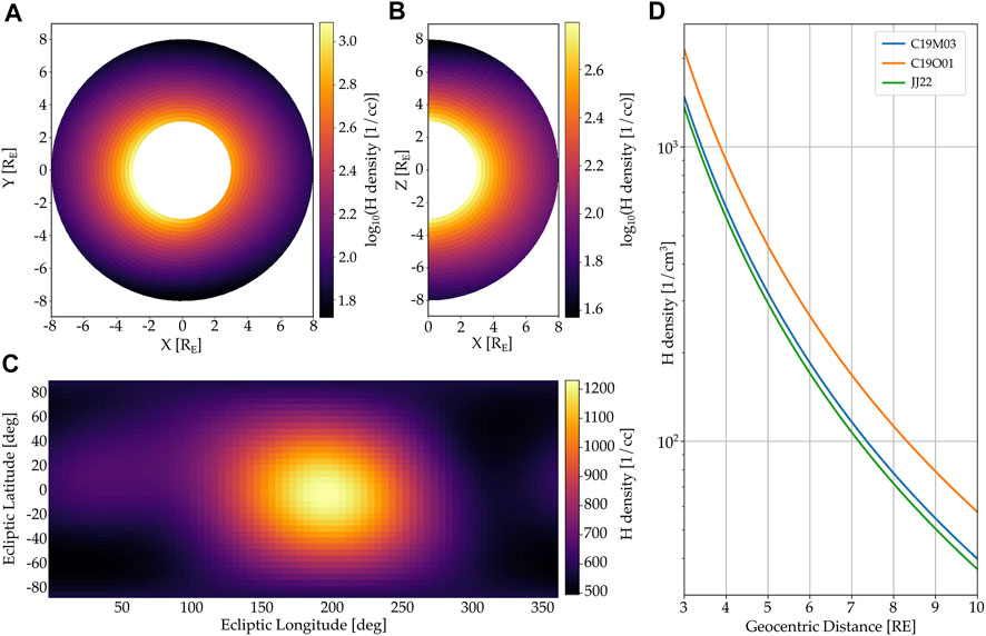
FIGURE 1. Visualization of H exospheric models included in the EXOSpy package. Panel (A) shows the equatorial plane of the 3-D H density profile derived by Zoennchen et al. (2015) for solar maximum conditions (Z15MAX). Panel (B) depicts the meridional (pole-to-pole) plane at the ecliptic longitude ϕ = 0° (noon). Panel (C) shows a spherical shell of H density at r = 5R_E. In addition, panel (D) shows a comparison between three 1-D H density models included in this package along the Sun-Earth line. All the plots use the Geocentric Solar Ecliptic (GSE) coordinate system, and radial distances are expressed in units of R_E.

2.2 Calculation of column-integrated lyman-alpha emission

Estimation of the column-integrated line of sight Ly-α intensity $(I(\widehat{n}))$ observed by a photometric instrument (e.g., a single-pixel photometer) requires information of its spatial position, the direction of its line-of-sight (LOS) vector and the exospheric volumetric emission rate (ɛ) which is generated by the interaction of solar Ly-α photons and atmospheric particles such as atomic H and molecular Oxygen (O₂).

To calculate $I(\widehat{n})$ within the terrestrial exosphere, EXOSpy solves the following equation (Bhattacharyya et al., 2017):

where $\widehat{n}$ represents the 3-D direction of the instrument LOS, the terms ɛ₀(l) and ɛ_m(l) are the volume emission rates due to single and multiple scattering of Ly-α photons by H atoms given in units of photons/cm³/sec, the terms ${\tau }_{\text{H}}(l)={\sigma }_H{\int }_0^L{n}_H(l)dl$ and ${\tau }_{{\text{O}}_2}(l)={\sigma }_{{\text{O}}_2}{\int }_0^L{n}_{{\text{O}}_2}(l)dl$ are the optical depth of the medium due to H atoms and O₂ molecules, σ_H represents the Ly-α photon scattering cross-section and ${\sigma }_{{\text{O}}_2}$ represents the Ly-α photon absorption cross-section by O₂. The line integral is evaluated from the beginning of the LOS (l = 0) to an appropriate upper boundary with a significant density of Ly-α emitters (l = L_max). Also, T(τ) is the Holstein function (Holstein, 1947) that estimates the photon transmission probability in a medium with optical depth τ(l) and is given by the relation

In addition, the term $\mathrm{\Psi }(\widehat{n})$ is the scattering function that estimates the probability of photon scattering in the direction $\widehat{n}$ and is formulated as

where $\theta (\widehat{n})$ is the angle between $\widehat{n}$ and the +X_GSE axis (Brandt and Chamberlain, 1959). The term $I_{IP}(\widehat{n})$ is the interplanetary Ly-α background, in units of Rayleigh, emitted by atomic H of interstellar origin.

The use of Eq. 1 requires volume emission rates for single and multiple scattering that can be estimated by a radiative transfer (RT) model. An RT model computes the single and multiple resonance scattering of photons by atmospheric particles and, for this purpose, requires solar photon flux and the cross-section of the particle-photon interaction as inputs to the model. For the analysis of the exosphere, the RT model uses three inputs: an H density profile (1-D for spherically symmetric distribution) to estimate the Ly-α photon scattering rate, an O₂ density profile to estimate the Ly-α photon absorption rate, and the incoming solar Ly-α flux usually expressed as irradiance at 121.56 nm in units of W/m². As a result, the RT model provides a spatial distribution of volume emission rates.

At high altitudes, where molecular oxygen is not found anymore (${\tau }_{{\text{O}}_2}=0$, $e^{-{\tau }_{{\text{O}}_2}}=1$), and the medium is optically thin (τ_H ≪ 1, T (τ_H) = 1), i.e., only single scattering of solar Ly-α occurs (ɛ_m = 0 and ɛ₀ = g* × n_H), Eq. 1 can be simplified as

where n_H(l) is the atomic H density in units of 1/cm³ and g* (also referred to as g-factor) is the scattering rate in units of photons/sec given by the relation

where f₀ represents the incoming line center solar Ly-α flux in photons/cm²/sec/Å, σ_H is the cross-section of the H Ly-α scattering cross section at line center, and δν_D is the Doppler width of the Ly-α emission line. Eq. 4 is only valid for the optically thin region of the exosphere, i.e., altitudes beyond 3 R_E geocentric distance.

Figure 2 depicts a block diagram that explains the steps to calculate line of sight column-integrated Ly-α intensities using EXOSpy. If the user selects a physics-based exospheric model that extends from 500 km altitude to 10 R_E geocentric distance, Eq. 1 is used to calculate intensities. As mentioned before, it requires volume emission rates for single and multiple scattering obtained from an RT model. This current version of EXOSpy does not include an RT model (white box in Figure 2), but it is considered to be part of a future release. To overcome this problem, we have included seven files with distributions of volume emission rates (ɛ₀ and ɛ_m) generated with Chamberlain-based H density profiles (see Section 2.1) and exobase parameters obtained from the NRLMSIS2.0 model corresponding to the equinox (March 20) from 2014 to 2020. This period represents solar maximum to solar minimum variations. In addition, O₂ densities, which typically extend up to ∼ 800 km altitude due to their smaller scale height in comparison to H, are also obtained from the NRLMSIS2.0 model. Solar irradiance data is included in each file and are retrieved from the LASP Interactive Solar Irradiance Datacenter (LISIRD) (https://lasp.colorado.edu/lisird/data/composite_lyman_alpha/). EXOSpy’s function Chamberlain implements the physics-based, 1-D Chamberlain model, which was used to generate the volume emission rates included in the package, and the function CalculateLOSfromVER implements Eq. 1 without considering Interplanetary Ly-α background.

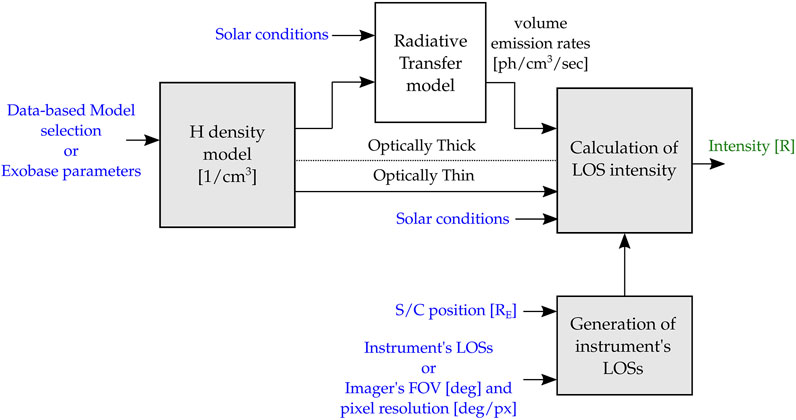
FIGURE 2. EXOSpy architecture to calculate column-integrated Ly-α intensities. Blue labels indicate user inputs, gray blocks are coded modules in EXOSpy and the white block indicate the module to be included in a future release of the package. Estimation of intensities for the optically thick region requires the use of a radiative transfer model which is not included in this version of EXOSpy; however, we provide a set of volume emission rate profiles for several solar conditions needed to estimate Ly-α intensities (see text for further details). EXOSpy provides a function to generate a synthetic imager when the FOV and pixel resolution are provided. Intensities values are generated in units of Rayleighs.

On the other hand, if the user selects a data-based exospheric model, Eq. 4 is used to calculate Ly-α intensity since these models are only valid for the optically thin region of the exosphere (see Table 1). In this case, the user should provide solar conditions as irradiance data which can be retrieved from LASP/LISIRD. EXOSpy’s function GenerateIntensityOpticallyThin implements Eq. 4 without considering Interplanetary Ly-α background.

Then, the user should provide a set of spacecraft positions and LOS directions in GSE coordinates to calculate the line of sight column-integrated Ly-α intensities. Also, EXOSpy allows the user to create a synthetic image comprised of individual LOSs when a FOV (in units of degrees) and a pixel resolution (in units of degrees/pixel) are provided.

Hence, EXOSpy calculates only the exospheric Ly-α emission which is the first term in the right hand side part of Eqs. 1, 4. Interplanetary Ly-α background (I_IP) can be retrieved from physics-based models (e.g. (Pryor et al., 1992)) or data provided by the Solar Wind ANisotropy (SWAN) instrument onboard the SOlar Heliospheric Observatory (SOHO) mission. The SOHO/SWAN instrument is located at Earth-Sun L1 point (Lagragian point), observing the interplanetary medium in Ly-α using a hydrogen cell. Its main product is a 1-day average all-sky map of the interplanetary Ly-α background.

2.3 Technical details of the EXOSpy package

The source code of EXOSpy is located in the following Github repository: https://github.com/gcucho/EXOSpy/. Also, a release of the package has been uploaded to a Zenodo repository and the download link can be found in (Cucho-Padin et al., 2022).

Furthermore, the package is part of the Python Package Index (PyPi) repository and its latest version (v2.3) can be installed to a personal computer using the command: pip install EXOSpy==2.3. For this, the user is required to have python 3.x and the pip application. Additionally, the following packages are needed: NumPy, SciPy, scikit-learn, and they will be installed automatically if they are not present in the user’s computer.

In this work, we have developed four examples to show how to use EXOSpy. These examples are available within the source code and their locations are indicated in the manuscript. The user can also go to our project’s website https://exospy.readthedocs.io/ for more information regarding these examples.

3 Applications

3.1 Validation of H exospheric models

Current and future models of exospheric density distributions can be assessed using EXOSpy and Ly-α radiance data from several space-based instruments such as the Geocorona Imager (GCI) onboard the Imager for Magnetopause-to-Aurora Global Exploration (IMAGE) mission, the Global UltraViolet Imager (GUVI) onboard the Thermosphere, Ionosphere, Mesosphere Energetics and Dynamics (TIMED) mission, and the LADs onboard the TWINS mission, among others.

We propose a validation methodology that is comprised of four steps: (i) select a Ly-α instrument and identify its orbit and instrument LOS(s), (ii) identify the exospheric region (optically thin or optically thick) observed by the instrument, (iii) set the testing exospheric model and calculate column-integrated Ly-α intensities using EXOSpy’s functions, and (iv) calculate the model performance. To demonstrate our approach, we show an example using TWINS/LAD measurements (step i). NASA’s TWINS mission is comprised of two satellites (TWINS1 and TWINS2) with a highly elliptical orbit, an apogee of 7.2 R_E, orbital precession of ≈1 year, and a 90° longitudinal separation between satellites to allow for stereoscopic observations. Each TWINS spacecraft has two LADs (single-pixel photometers) that rotate 180° around a constant nadir pointing vector (McComas et al., 2009). TWINS radiance and ephemeris data are publicly available in NASA’s Space Physics Data Facility (SPDF) repository. Panel (A) in Figure 3 shows TWINS1/LAD1 observations for three rotations acquired on 11 June 2008, 08:20 UT. These observations have been pre-processed to remove stellar contamination and interplanetary Ly-α background as per the procedure detailed in (Cucho-Padin and Waldrop, 2018). The black line indicates the TWINS1 orbit, the green lines are LAD1’s LOSs, and the blue arrow indicates the initial clockwise rotation of the LAD instrument around the nadir vector. Due to the LOSs viewing geometry, these observations serve to evaluate exospheric models beyond 3 R_E geocentric distance, i.e., optically thin region (step ii). EXOSpy enables the user to input a new exospheric model as spherical harmonic coefficients or as discrete 3-D spatial locations in GSE spherical coordinates using the class exosgrid. In this example, we use the model developed by Zoennchen et al. (2015) for solar minimum conditions, which is included in the package (Z15MIN). Then, we estimated the line of sight column-integrated Ly-α intensities using EXOSpy’s function $\mathtt{G}\mathtt{e}\mathtt{n}\mathtt{e}\mathtt{r}\mathtt{a}\mathtt{t}\mathtt{e}\mathtt{I}\mathtt{n}\mathtt{t}\mathtt{e}\mathtt{n}\mathtt{s}\mathtt{i}\mathtt{t}\mathtt{y}\mathtt{O}\mathtt{p}\mathtt{t}\mathtt{i}\mathtt{c}\mathtt{a}\mathtt{l}\mathtt{l}\mathtt{y}\mathtt{T}\mathtt{h}\mathtt{i}\mathtt{n}$. Panel (B) in Figure 3 shows a comparison between the calculated intensities based on Z15MIN model in blue line (step iii) and the actual data measured by the TWINS1/LAD1 instrument on 19 June 2008, in the dashed red line. Finally, these values can be evaluated using several performance indicators such as minimum square error or the Pearson correlation coefficient, among others (step iv). Panel (B) shows an evident disagreement between TWINS/LAD observations and calculated intensities in the minima regions that are possibly associated with the multi-day approach used to generate this exospheric model. Specifically, Z15MIN was implemented using Ly-α observations during the periods June 19–21, 2008, and June 19–21, 2010. The intensities shown in the blue line were obtained using Eq. 4 and only considering solar flux for 19 June 2008 (used in Eq. 5). Hence, the exospheric model can reflect the average behavior of density distributions for several days in two different years and may exclude the formation of daily structural patterns in the density distributions. Nevertheless, further analysis should be done to draw firm conclusions regarding the validity of this model.

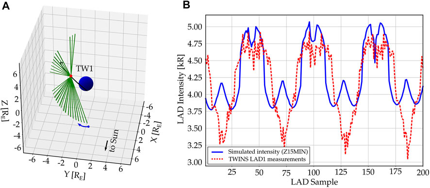
FIGURE 3. Simulation of TWINS1/LAD1 observations of the optically thin exosphere. In Panel (A), the black line indicates TWINS1 (TW1) orbit, green lines are LAD’s LOSs rotating 180° around a nadir pointing vector, and the blue arrow indicates the initial direction of rotation. In Panel (B), the blue line shows the calculated intensity for each LOS using the Z15MIN model and Eq. 4, and the dashed red line shows the actual data from TWINS1/LAD1 instrument.

The python notebook Example2. ipynb uploads the pre-processed ephemeris and attitude data from TWINS1/LAD1 and shows the use of EXOSpy’s functions to generate column-integrated Ly-α intensities. The reader can access the file in https://github.com/gcucho/EXOSpy/blob/main/Examples/Example2.ipynb.

3.2 Estimation of exospheric contamination in current space-based UV instruments

Observations of extra-terrestrial bodies in UV might be contaminated by the bright exospheric emission, and its removal or avoidance is crucial for the correct analysis of the measurements.

To demonstrate how EXOSpy may help quantify this background emission, we estimate the Ly-α intensities as seen from a Low earth Orbit (LEO) satellite. Specifically, we simulate the orbit and viewing geometry of the TIMED/GUVI instrument, which are similar to those of the HST mission. Panel (A) in Figure 4 shows in blue line the orbit of the satellite within the XY ecliptic plane at an altitude of 600 km (optically thick region). Red dots indicate positions when the spacecraft acquires data, and green lines are examples of measurements’ LOSs only for two positions for better visualization. TIMED/GUVI is a spectrograph with a rotating mirror that allows LOS observations of the earth’s limb from look angles (LA) that range from 0 to 20°. A LOS has LA = 0° when its direction is perpendicular to the zenith and LA $>0$ degrees when its direction is closer to the earth. The satellite location is represented by the angle between + X_GSE axis and the zenith, also referred to as the solar zenith angle (SZA). For each satellite position (red dot), we simulated LOSs covering 20° LA with a 1-degree resolution. Then, we calculate the column-integrated Ly-α intensity using EXOSpy’s function CalculateLOSfromVER as well as the volume emission rates for the optically thick region during solar minimum conditions (year 2020).

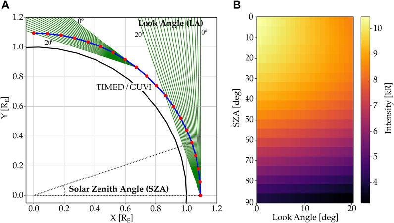
FIGURE 4. Simulation of TIMED/GUVI observations of the optically thick exosphere. Panel (A) shows the trajectory of the GUVI instrument projected to the XY ecliptic plane as a blue line. Red dots indicate the position of the satellite where measurements are carried out. Green lines are LOSs for several look angles, LA ∈ [0, 20] degrees. Panel (B) shows the calculated intensities by EXOSpy using the volume emission rate for the year 2020, i.e., during solar minimum conditions.

Panel (B) in Figure 4 shows the resulting Ly-α intensities. Two typical features of exospheric emission are shown in this plot. First, the Ly-α intensity is reduced as the satellite transits from dayside (SZA = 0°) to dusk (SZA = 90°) due to the thicker atmosphere the solar Ly-α flux encounters on its path, ultimately resulting in fewer photons reaching the dusk/nightside region. Second, the presence of denser molecular oxygen at low altitudes absorbs Ly-α photons such that LOSs with smaller tangential distances may produce lower intensities. For instance, for a satellite position SZA = 0°, a LOS with LA = 0° yields ∼ 10 kR while a LOS with LA = 20° yields ∼ 8 kR since its path crosses lower down in the atmosphere, which has a larger amount of O₂ molecules. The python notebook Example3. ipynb shows the use of EXOSpy’s functions to generate TIMED/GUVI’s LOSs and their column-integrated Ly-α intensities. The reader can access the file in https://github.com/gcucho/EXOSpy/blob/main/Examples/Example3.ipynb.

3.3 UV instrument design

The EXOSpy package can be used as part of the designing process of space-based UV instruments for several mission objectives such as estimation of exospheric H density distributions or observation of extra-terrestrial bodies in FUV wavelengths other than Ly-α.

Here we describe how the EXOSpy package can be used to design a wide FOV imager to observe the exosphere in Ly-α. This task typically aims to determine several optical parameters such as FOV (in degrees), pixel resolution (in degrees/pixel), sensor responsivity at Ly-α (in counts/sec/R), integration time (in seconds), the optimal ephemeris, and the optimal pointing viewing geometry. In this case, the designing methodology is an iterative process wherein an initial set of the above-listed parameters are used to generate an image that is then evaluated against certain requirements such as signal-to-noise ratio (SNR) or its capability to yield additional scientific products, e.g., H densities with lower uncertainty. If these requirements are not met, the parameters are modified, and a new iteration is performed. For this application, we simulate an image to observe the optically thin region of the exosphere with the following parameters: a square FOV of 18°, a pixel resolution of 18/72°/pixel, a geosynchronous orbit with a radius of 6.6 R_E over the ecliptic plane, and an anti-sunward pointing viewing geometry. Panel (A) in Figure 5 shows a simulation of this instrument where the red dots indicate two acquisition periods, green sectors show the square FOV, and the black line represents the orbit. To generate synthetic intensities, we select H density distributions during solar maximum conditions, i.e., Z15MAX model (see Table 1). The solar irradiance used in this example was 0.0086 W/m² obtained from LISIRD/LASP website for 20 June 2012. Panels (B) and (C) show the resulting 72 × 72 pixel image for each satellite position. The python notebook Example4. ipynb shows the use of EXOSpy’s function to generate a wide field image for the different pixel LOSs by calculating their corresponding column-integrated Ly-α intensities. The reader can access the file in https://github.com/gcucho/EXOSpy/blob/main/Examples/Example4.ipynb. It is worth noting that these images show a dawn/dusk asymmetry in the intensities, which, at this altitude, is directly associated with an asymmetric distribution of H densities. In addition, we adopt a sensor responsivity at Ly-α equal to 5 × 10^–3 counts/sec/R (typical for a CCD imaging sensor) and an integration time of 10 min. As a result, the number of digital counts in the images range from ∼5100 to ∼7200 counts. Assessment of this parameter setting can be done using a threshold SNR. In optical systems, the main source of noise is the Poisson-distributed shot noise which, in turn, simplifies the derivation of the measurement’s SNR to $\sqrt{N}$, where N is the number of digital counts. Hence, the SNR for these images range from ∼71 to ∼84.

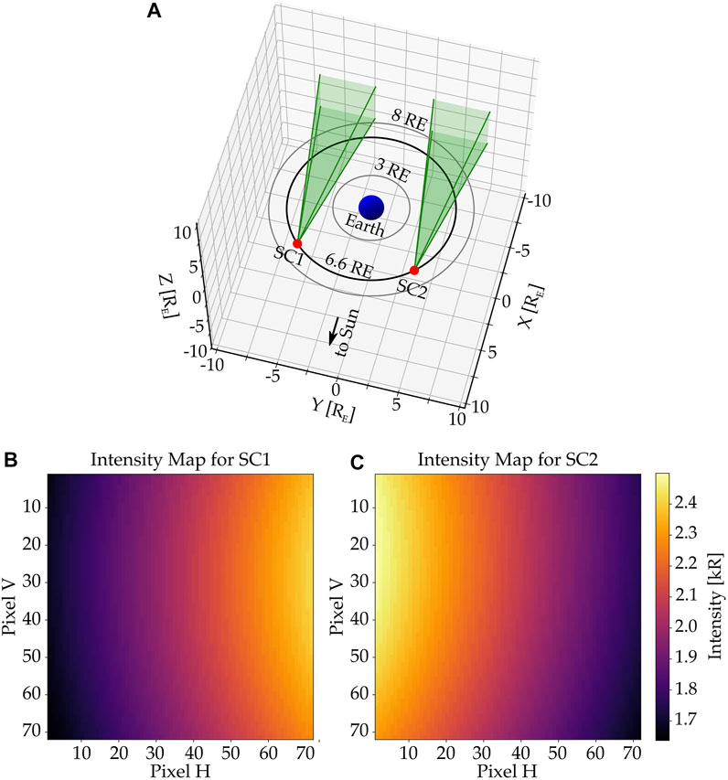
FIGURE 5. Simulation of a wide FOV imager to observe the optically thin exosphere. Panel (A) shows the viewing geometry for an spacecraft located in a geosynchronous orbit with radius 6.6 R_E. Red dots indicate the positions where the imager acquire an image. See the text for further details of optical parameters. Panels (B,C) show the calculated intensities by EXOSpy using the 3-D H model Z15MAX (valid only from 3 to 8 R_E).

Unlike spectrograph-based instruments that can resolve narrow wavelengths bands, imagers rely on optical filters or a combination of them to generate a narrow responsivity function. Nevertheless, imagers are still the best option to obtain a global view of the target. For example, future astrophysics missions might be interested in observing very distant galaxies in Ly-α using imagers. Depending on the galaxy’s distance and its velocity with respect to the observer, they may be red-shifted (z) from 121.56 nm. For instance, observation of a target with a red-shift parameter of z = 0.2 indicates that an emitted 121.56 nm photon would be observed as 145.87 nm at earth. The proximity of these wavelengths requires an effective selection of optical filters to generate a responsivity function able to suppress the exospheric Ly-α emission. For this purpose, an accurate specification of this bright emission under different solar conditions is required. This task can be achieved using the similar approach presented in Section 3.2 to estimate column-integrated Ly-α emissions for a given satellite position and instrument’s LOSs.

4 Summary and future work

In this work, we have developed EXOSpy, an open-source python-based package to explore current terrestrial exospheric models and calculate their Ly-α emission. Through examples provided in this project, we demonstrate the capabilities of EXOSpy (i) to validate exospheric models with actual Ly-α radiance data, (ii) to estimate exospheric contamination that may affect extra-terrestrial observations, and (iii) to support UV instrument design.

Future development of the EXOSpy package includes (i) the implementation of an open-source 3-D Radiative Transfer model that can automatically provide volume emission rates for a given 3-D H density profile, (ii) the capability for directly downloading actual Ly-α data from TWINS/LAD, IMAGE/GEO and TIMED/GUVI instruments and subsequent comparison with synthetically-generated column-integrated Ly-α measurements, and (iii) the capability for downloading 1-day averaged interplanetary Ly-α background from the SOHO/SWAN instrument.

Data availability statement

The EXOSpy’s source code and Jupyter notebook used to generate figures in this paper can be found https://zenodo.org/record/7245359 in Zenodo. TWINS Lyman-alpha data are publicly available through the NASA Space Physics Data Facility.

Author contributions

GC-P conceptualized this project, developed the python package and wrote the manuscript. DB co-developed the python package and reviewed the manuscript, DS supervised the work, secured funding, and reviewed the manuscript. HC provided feedback regarding the validation of exospheric models and reviewed the manuscript. AY provided feedback regarding contamination in astrophysics applications and reviewed the manuscript. DA provided feedback regarding UV instrument design and reviewed the manuscript. All authors contributed to the article and approved the submitted version.

Funding

NASA Cooperative Agreement 80NSSC21M0180G: Partnership for Heliophysics and Space Environment Research (NS) NASA Heliophysics United States Participating Investigator Program under Grant WBS516741.01.24.01.03 WBS516741.01.24.01.03 (DS).

Acknowledgments

We acknowledge the support from the International Space Science Institute on the ISSI team 492, titled “The earth’s Exosphere and its Response to Space Weather”. Also, HC gracefully acknowledges support from the NASA grants, 80NSSC20K1670 and 80MSFC20C0019.

Conflict of interest

The authors declare that the research was conducted in the absence of any commercial or financial relationships that could be construed as a potential conflict of interest.

Publisher’s note

All claims expressed in this article are solely those of the authors and do not necessarily represent those of their affiliated organizations, or those of the publisher, the editors and the reviewers. Any product that may be evaluated in this article, or claim that may be made by its manufacturer, is not guaranteed or endorsed by the publisher.

References

Bailey, J., and Gruntman, M. (2011). Experimental study of exospheric hydrogen atom distributions by Lyman-alpha detectors on the TWINS mission. J. Geophys. Res. Space Phys. 116, 1–9. doi:10.1029/2011JA016531
Baliukin, I. I., Bertaux, J.-L., Quémerais, E., Izmodenov, V. V., and Schmidt, W. (2019). SWAN/SOHO Lyman-alpha mapping: The hydrogen geocorona extends well beyond the Moon. J. Geophys. Res. Space Phys. 124, 861–885. doi:10.1029/2018JA026136
Bhattacharyya, D., Clarke, J., Bertaux, J.-L., Chaufray, J.-Y., and Mayyasi, M. (2017). Analysis and modeling of remote observations of the Martian hydrogen exosphere. Icarus 281, 264–280. doi:10.1016/j.icarus.2016.08.034
Bourrier, V., Ehrenreich, D., Lecavelier des Etangs, A., Louden, T., Wheatley, P. J., Wyttenbach, A., et al. (2018). High-energy environment of super-Earth 55 cancri e - i. far-uv chromospheric variability as a possible tracer of planet-induced coronal rain. A&A 615, A117. doi:10.1051/0004-6361/201832700
Brandt, J. C., and Chamberlain, J. W. (1959). Hydrogen radiation in the night sky. Astrophys. J. 130, 670–682.
Carruthers, G. R., Page, T., and Meier, R. R. (1976). Apollo 16 Lyman alpha imagery of the hydrogen geocorona. J. Geophys. Res. 81, 1664–1672. doi:10.1029/ja081i010p01664
Chamberlain, J. W. (1963). Planetary coronae and atmospheric evaporation. Planet. Space Sci. 11, 901–960. doi:10.1016/0032-0633(63)90122-3
Connor, H. K., and Carter, J. A. (2019). Exospheric neutral hydrogen density at the nominal 10 RE subsolar point deduced from XMM-Newton X-Ray observations. J. Geophys. Res. Space Phys. 124, 1612–1624. doi:10.1029/2018JA026187
Cucho-Padin, G., Ferradas, C., Waldrop, L., and Fok, M. C. H. (2020). Understanding the role of exospheric density in the ring current recovery rate. AGU Fall Meet. Abstr. 2020, SM037.
Cucho-Padin, G., Kameda, S., and Sibeck, D. G. (2022). The Earth’s outer exospheric density distributions derived from procyon/laica uv observations. J. Geophys. Res. Space Phys. 127, e2021JA030211. doi:10.1029/2021JA030211
Cucho-Padin, G., and Waldrop, L. (2019). Time-dependent response of the terrestrial exosphere to a geomagnetic storm. Geophys. Res. Lett. 46, 11661–11670. doi:10.1029/2019gl084327
Cucho-Padin, G., and Waldrop, L. (2018). Tomographic estimation of exospheric hydrogen density distributions. J. Geophys. Res. Space Phys. 123, 5119–5139. doi:10.1029/2018ja025323
Emmert, J. T., Drob, D. P., Picone, J. M., Siskind, D. E., Jones, M., Mlynczak, M. G., et al. (2021). NRLMSIS 2.0: A whole-atmosphere empirical model of temperature and neutral species densities. Earth Space Sci. 8, e2020EA001321. doi:10.1029/2020ea001321
Esposito, L. W., Barth, C. A., Colwell, J. E., Lawrence, G. M., McClintock, W. E., Stewart, A. I. F., et al. (2004). The cassini ultraviolet imaging spectrograph investigation. Space Sci. Rev. 115, 299–361. doi:10.1007/s11214-004-1455-8
Fairfield, D. H. (1971). Average and unusual locations of the Earth’s magnetopause and bow shock. J. Geophys. Res. 76, 6700–6716. doi:10.1029/JA076i028p06700
Holstein, T. (1947). Imprisonment of resonance radiation in gases. Phys. Rev. 72, 1212–1233. doi:10.1103/physrev.72.1212
Ilie, R., Liemohn, M. W., Toth, G., and Skoug, R. M. (2012). Kinetic model of the inner magnetosphere with arbitrary magnetic field. J. Geophys. Res. Space Phys. 117, 7189. doi:10.1029/2011ja017189
Jung, J., Connor, H. K., Carter, J. A., Koutroumpa, D., Pagani, C., and Kuntz, K. D. (2022). Solar minimum exospheric neutral density near the subsolar magnetopause estimated from the xmm soft x-ray observations on 12 november 2008. J. Geophys. Res. Space Phys. 127, e2021JA029676. doi:10.1029/2021ja029676
Krall, J., Glocer, A., Fok, M.-C., Nossal, S. M., and Huba, J. D. (2018). The unknown hydrogen exosphere: Space weather implications. Space weather. 16, 205–215. doi:10.1002/2017SW001780
McComas, D. J., Allegrini, F., Baldonado, J., Blake, B., Brandt, P. C., Burch, J., et al. (2009). The two wide-angle imaging neutral-atom spectrometers (TWINS) NASA mission-of-opportunity. Space Sci. Rev. 142, 157–231. doi:10.1007/s11214-008-9467-4
Pryor, W. R., Ajello, J. M., Barth, C. A., Hord, C. W., Stewart, A. I. F., Simmons, K. E., et al. (1992). The Galileo and Pioneer Venus ultraviolet spectrometer experiments: Solar Lyman-alpha latitude variation at solar maximum from interplanetary Lyman-alpha observations. Astrophysical J. 394, 363. doi:10.1086/171589
Waldrop, L., and Paxton, L. J. (2013). Lyman-alpha airglow emission: Implications for atomic hydrogen geocorona variability with solar cycle. J. Geophys. Res. Space Phys. 118, 5874–5890. doi:10.1002/jgra.50496
Werner, S., Keller, H., Korth, A., and Lauche, H. (2004). Uvis/hdac lyman-alpha observations of the geocorona during cassini’s Earth swingby compared to model predictions. Adv. Space Res. Ionos. Atmos. Incl. CIRA 34, 1647–1649. doi:10.1016/j.asr.2003.03.074
Wood, B. E., Redfield, S., Linsky, J. L., Müller, H.-R., and Zank, G. P. (2005). Stellar lyα emission lines in the Hubble space telescope archive: Intrinsic line fluxes and absorption from the heliosphere and astrospheres. Astrophysical J. Suppl. Ser. 159, 118–140. doi:10.1086/430523
Youngblood, A., France, K., Loyd, R. O. P., Linsky, J. L., Redfield, S., Schneider, P. C., et al. (2016). The muscles treasury survey. II. Intrinsic LYαAND extreme ultraviolet spectra of K and M dwarfs with exoplanets. Astrophysical J. 824, 101. doi:10.3847/0004-637x/824/2/101
Zoennchen, J. H., Connor, H. K., Jung, J., Nass, U., and Fahr, H. J. (2022). Terrestrial exospheric dayside h-density profile at 3–15 rE from uvis/hdac and twins lyman-α data combined. Ann. Geophys. 40, 271–279. doi:10.5194/angeo-40-271-2022
Keywords: terrestrial exosphere, FUV, lyman-alpha, atomic hydrogen, python
Citation: Cucho-Padin G, Bhattacharyya D, Sibeck DG, Connor H, Youngblood A and Ardila D (2023) EXOSpy: A python package to investigate the terrestrial exosphere and its FUV emission. Front. Astron. Space Sci. 10:1082150. doi: 10.3389/fspas.2023.1082150
Received: 27 October 2022; Accepted: 11 January 2023;
Published: 24 January 2023.
Edited by:
Angeline G. Burrell, United States Naval Research Laboratory, United StatesReviewed by:
Brian Harding, University of California, Berkeley, United StatesAlla V. Suvorova, National Central University, Taiwan
Copyright © 2023 Cucho-Padin, Bhattacharyya, Sibeck, Connor, Youngblood and Ardila. This is an open-access article distributed under the terms of the Creative Commons Attribution License (CC BY). The use, distribution or reproduction in other forums is permitted, provided the original author(s) and the copyright owner(s) are credited and that the original publication in this journal is cited, in accordance with accepted academic practice. No use, distribution or reproduction is permitted which does not comply with these terms.
*Correspondence: Gonzalo Cucho-Padin, gonzaloaugusto.cuchopadin@nasa.gov