Relationship between geomagnetic storms and occurrence of ionospheric irregularities in the west sector of Africa during the peak of the 24th solar cycle

1 Introduction

The impact of the solar events on specific technologies that rely on the ionospheric conditions is an important subject of investigation. The nighttime ionospheric disturbance and fluctuations represented by the difference in total electron content (ΔTEC) from its quiet mean and the rate of change of total electron content (ROT), respectively, affect technological events such as communication, especially trans-ionospheric communication (Hughes, 2009). The ionospheric disturbance may be affected by the geoeffectiveness of solar events. The geoeffectiveness of the solar events, such as the coronal mass ejections (CMEs) and the solar flares can be observed using the geomagnetic indices, such as auroral electrojet (AE) index, disturbance storm time (Dst) index, ASY/SYM index, and Kp and ap/Ap indices, among others, as proxies (Badruddin & Falak, 2016). According to Campbell (1979), the geomagnetically active time starts when the solar wind that carries evidence of the Sun’s disturbances encounters the boundary region above the Earth’s magnetic field extension into space. The boundary region, in this case, is of the Earth’s magnetosphere, particularly along its dayside interface with the solar wind (the magnetopause) and at the transition between open and closed magnetic field lines in the magnetic tail (Burch et al., 2016). The composition of the particles’ density, velocity, and field direction of the solar wind determines the dynamics that can compress this dayside boundary of the magnetospheric cavity, causing magnetopause currents to flow in a manner that causes an increase of the magnetic field at the geosphere in a direction parallel to the geomagnetic axis. This initial rise of the magnetic field manifests as an increase in the positive direction of the positive Dst index. The continuing interactions of the solar wind particles at the Earth’s magnetotail region at the night side of the Earth come along with energetic particles in the near-Earth magnetosphere, forming the so-called ring current around the Earth. This ring current causes major fluctuations of the magnetic field within the reach of the nearby observatory’s magnetograms (Kendall et al., 1966). A slow decay of this ring current may be detectable for several days after the disturbance period onset, as a storm recovery phase. The geomagnetic storms are the major indicators of geoeffectiveness (Gopalswamy, 2009; Richardson & Cane, 2011). However, to measure some impact of the solar events on technology, we investigate the correlation between geomagnetic storm index, disturbance storm time index, Dst, and ionospheric irregularity occurrences, in our case using the rate of change of TEC index (ROTI).

Geomagnetic storms at times may occur concurrently with ionospheric storms (Rama Rao et al., 2009). During a geomagnetic storm, the magnetic field of the Earth can at times decrease to −300 nT or even less. The geomagnetic storm caused by a solar flare usually starts off with a sudden increase in the Earth’s magnetic field at the initial phase and is called a sudden commencement (SSC) storm (Perreault & Akasofu, 1978). The impact of the geomagnetic storms has been studied using total electron content (TEC) data derived from the Global Positioning System (GPS). The data are used to study the ionospheric disturbances such as scintillations among others (Mendillo et al., 2000).

It is widely believed that scintillations and plasma bubbles can only occur at nighttime (Miller et al., 2009). Xie et al. (2020) investigated the unexpected high occurrence of daytime F-region backscatter plume structures over low-latitude Sanya and their possible origin. Their observations revealed that the daytime F-region echoes, which are caused by the plume structures consisting of field-aligned irregularities, occur with an unexpected high occurrence of ∼13% in June solstice of solar minimum. One possible reason for the observation of the daytime ionospheric disturbance as observed by Xie et al. (2020) is the plume structure and associated irregularities which were freshly generated at daytime. Li et al. (2018) reported a case of the daytime plume irregularity structure triggered by rocket exhaust-induced ionosphere holes over low latitudes. The structure was initially observed as a thin layer and then evolved into a vertical structure. For the daytime structure in their study, no preceding thin layer was detected. There was also no ionospheric hole detected by ground-based total electron content receivers, suggesting that the daytime plume structures might not be freshly generated at daytime. The second possible reason for such an occurrence is that the daytime F-region irregularities, as a result of fossils of equatorial plasma bubbles (EPBs), were generated at the previous night. The residual effect of the previous night’s EPB could be observed as a daytime F-region irregularity. At the topside ionosphere, plasma density depletions were observed both at daytime and previous night by satellite in situ measurements (Huang et al., 2014 and Kil et al., 2019).

The aim of the present study is to show the relationship between geomagnetic storm occurrences and the ionospheric irregularities during the peak of the 24th solar cycle. This gives an in-depth knowledge of the dynamics of the SC 24, given that it has one of the lowest sunspot numbers since 1874 (Veronig et al., 2021). The next peak (of the 25th solar cycle) is expected in July 2025.

This study shows a wider view of the relationships between occurrences of ionospheric irregularities as determined using ROTI and geomagnetic storms during the peak of solar cycle (SC) 24. Knowing the drivers of the geomagnetic storms, whether CMEs or CIRs, helps us know the ones which creates the most impact on technology. We focus particularly on the year 2012, which is one of the peak years of the solar cycle. In Section 2, we explain the data used, their sources, and the methodology; in Section 3, we explain the results and analysis of the results; in Section 4, we feature discussions; and Section 5 is conclusion.

2 Data and methodology

The Global Navigation Satellite Systems (GNSS) data for the work were obtained from the Nigerian Permanent GNSS Network (NIGNET) receiver, specifically stationed in Abuja. The website of the data archive is www.nignet.net. At the time of writing of this paper, the website was down. The data for some of the stations on the network were downloaded from the websites of the African Geodetic Reference Frame (AFREF; http://afrefdata.org) and the Calibrated GNSS TEC Service of the International Centre for Theoretical Physics (ICTP; http://arplsrv.ictp.it/). The code of the station used is OCGF; the geographic coordinates were latitude: 9.03° and longitude: 7.49°; and geomagnetic coordinates were observed as latitude: −1.60° and longitude: 79.50°. The receivers of all NIGNET data in Nigeria are listed in Table 1. The receivers majorly received data from satellites on the GPS and Global Navigation Satellite System (GLONASS) constellations.

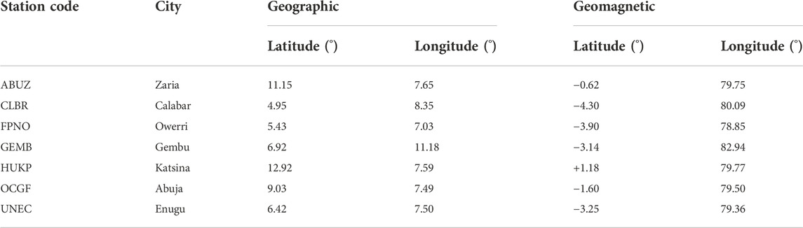
TABLE 1. NIGNET receiver stations. The latitudes are positive for north and negative for south, while the longitudes are positive for east.

The geomagnetic data for the study were obtained from the World Data Center in Kyoto (http://swdcdb.kugi.kyoto-u.ac.jp/dstdir/) for the entire period of the study. The resolution of the disturbance storm time (Dst) was 1 hour. The data used for this research covered the period ranging from January 2012 to December 2012. During that period, a total of 56 geomagnetic storm events were considered for the study. The Dst indices for the events ranged from a minimum of −145 to −30 nT.

For the purposes of the identification of the geomagnetic storm drivers, we used CIR catalog from 2001 to 2015 from the site https://www.helcats-fp7.eu/catalogues/wp5_cat.html and the CME catalog within the period 2001–2020 from the site http://www.srl.caltech.edu/ACE/ASC/DATA/level3/icmetable2.htm.

We used the procedure described by Nishioka et al. (2008) to check the occurrence of plasma bubbles on the data. Slant TEC (STEC) was derived for every 30 s from GNSS data using software developed by Seemala and Valladares (2011). STECs were computed for all ray paths between the satellites and the receivers whose elevation angles were greater than 30°. The elevation angle cutoff was adopted in order to eliminate the multi-path effects.

GPS Scintillation Network Decision Aid (SCINDA) TEC data were obtained from the Air Force Research Laboratory (AFRL) data archive, http://capricorn.bc.edu/scinda/ihy, with permission. The data are available only with prior permission. The receivers available in Nigeria are listed in Table 2. Out of all these GPS SCINDA receivers, the AFRL-SCINDA data archive, access to which we were given, stores data as images in the graphics interchange format (GIF) only.

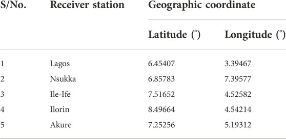
TABLE 2. GPS SCINDA receiver stations available in Nigeria.

2.1 The rate of change of total electron content

Different researchers have used different indices to study ionospheric scintillations (Oladipo & Schüler, (2013) and references therein). Oladipo & Schüler (2013) and Wanninger (1993) utilized the rate of change of TEC (ROT) given in Eq. 1 to compute the occurrence of ionospheric irregularities.

where Δt is the change in time in minute, $ROT$ is in TECU per minute, and ΔTEC is defined by subtracting each TEC from its previous value. In this work, we used a similar formula as given in Eq. 1.

2.2 The rate of change of total electron content index

Scintillation occurs only when the irregularity sizes of the plasma depletions are within the Fresnel scale size (Basu et al., 1999). ROTI represents the signature of irregularity scale sizes in thousands of meters. A 5 min ROTI can detect 30 km scale irregularities when the structure moves with a velocity of 100 m·s⁻¹ at the altitude of the ionospheric pierce point (IPP) (Buhari et al., 2014). To recognize small-scale fluctuations, the 5 min standard deviation of ROT was computed. This value is called the rate of TEC change index (ROTI) (Pi et al., 1997; Mendillo et al., 2000; Nishioka et al., 2008). ROTI has been regularly used to investigate ionospheric fluctuations. The maximum value of ROTIs derived from individual GNSS signals was used as the ROTI value for the 5 min period. In order to detect plasma irregularities, we computed one 30 min ROTI from six values of 5 min ROTI. According to Nishioka et al. (2008), 5 min ROTI also has large values when there are incidences of errors in TEC measurements.

For the GNSS data, if plasma irregularities, especially plasma bubbles are detected in any of the stations, then the day is considered one with a plasma irregularity or bubble occurrence that can also be witnessed on the airglow image.

Pi et al. (1997) suggested that an index for the rate of change of TEC can be determined from the standard deviation of the ROT in a 5-min interval. It is given by Eq. 2.

ROTI is a good indicator of the existence of ionospheric irregularities, and ROTI ≥ 0.5 indicates the occurrence of irregular ionospheric activities relevant to ionospheric scintillation (Yang & Liu, 2016).

Ma & Maruyama (2006) defined the levels of ROTI into five distinct categories: 0 < ROTI < 0.5; 0.5 < ROTI < 1; 1 < ROTI < 1.5; 1.5 < ROTI < 2; and ROTI ˃ 2. The final category is the loss of channel lock for a receiver–satellite pair. It could be the loss of lock occurred to both L1 and L2 signals. In their work, most of the cases were the loss of L2 signal lock, while only pseudorange was measured for L1.

2.3 S4 index

The data obtained from the NIGNET receivers could not be used to obtain the S4 indices. The data cadence of two data points per minute, which is 0.03333 Hz, was way lower than 50 Hz required for the S4 determination (Kapil et al., 2022 and references therein). A special ionospheric scintillation monitoring-GPS receiver is required to record the S4 index, as it is derived from the high rate amplitude of the received signal. Thus, the regular dual GNSS frequency that most commonly records the pseudorange and phase observables at 30-s or 1-s sampling interval cannot be used to derive the S4 index (Kapil et al., 2022).

The computation of the scintillation index, S4, which is defined as the normalized variance of the intensity of the signal (Yeh & Liu, 1982), is given in Eq. 3. This S4 index measures the intensity of amplitude fluctuations caused by radio signals transcending the ionosphere from satellites to Earth receiver stations. This index measures rapid variations in the amplitude of radio wave signals caused by small-scale structures of ionospheric irregularities in the ionosphere. The GPS ISM receivers directly calculate the S4 index from the raw data sampled at 50 Hz, as given in Eq. 3, which is implemented in the receiver firmware (Rama Rao et al., 2009). Very severe scintillation conditions can prevent a GPS receiver from locking on to the received signal and can severely reduce the accuracy of position estimates. Thus, scintillation conditions can reduce the accuracy of positioning results (Kapil et al., 2022).

The S4 values measured from each of the PRNs representing values at each of the ionospheric pierce point (IPP) of that PRN to represent the station where the GPS receiver is installed could be deduced from the plots of S4.

3 Results and analysis

3.1 Quantification of ionospheric irregularities using the rate of change of total electron content index

Figure 2 shows sample plots of ROTI during the year 2012. They are ROTI plots for 13 April, 15 July, 9 October, and 1 October of the same year. The geomagnetic storms in the sampled dates were of minimum values, which were −60, −139, −122, and −109 nT, respectively. The maximum ROTI for the days were 1.4, 0.24, 0.9, and 0.33 TECU/min, respectively.

It is evident that the ionospheric irregularities only took place in at local nighttime. The rest of the daytime had very low values of ROTI. The nominal values of ROTI during the undisturbed times were 0.2 TECU/min. The maximum values would be in excess of 0.25 TECU/min and obviously higher than the nominal values for the day.

In all cases, the ROTI peaks were observed at about 19:00 h local time (which was 20:00 h universal time). The magnitude of the geomagnetic index did not quite match the irregularities as registered. As examples, in Figure 2A, the geomagnetic index had a magnitude of −60 nT, and the ROTI was 1.4 TECU/min, which was very significant. In Figure 1B, however, the geomagnetic index had a magnitude of −139 nT, which is strong, and the ROTI was only 0.24 TECU/min. Similar trends are seen in Figures 1C,D.

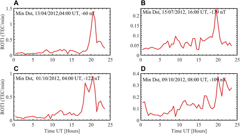
FIGURE 1. Variation of ROTI collectively computed from all stations in Table 1, with the time of the day, during geomagnetically active days. The UT in the time scale is one (1) hour behind Nigerian local time (LT). Dst, Min indices ranged from −139 to −60 nT. The ROTI was calculated at a 30-min interval. (A) shows variation ROTI with Dst, Min of −60 nT on 13/04/2012, 04:00 UT, (B) shows variation ROTI with Dst, Min of −139 nT on 15/07/2012, 16:00 UT, (C) shows variation ROTI with Dst, Min of −122 nT on 01/10/2012, 04:00 UT and (D) shows variation ROTI with Dst, Min of −109 nT on, 09/10/201208:00 UT.

3.2 Periods associated with the rate of change of total electron content index values

The obtained PSD for the hourly ROTI values is shown in Figure 2. The figure reveals prominent peaks on the PSD profiles.

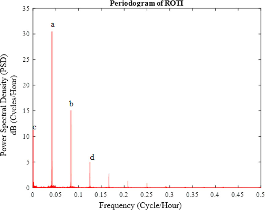
FIGURE 2. Periodogram of hourly ROTI values for the year 2012. The peaks marked (A–D) are, respectively, centered at 0.04169, 0.08331, 0.00024, and 0.12500 cycles/hour.

The most prominent peaks on the PSD profile are marked with the letters a–d, in order of decreasing power spectral density. As can be seen from the figure, an analysis of the PSD profile shows that the peaks marked a–d are, respectively, centered at 0.04169, 0.08331, 0.00024, and 0.12500 cycles/hour (on the horizontal axes). These values represent the most dominant frequencies in the PSD profile, and their reciprocals (in hours) represent the most dominant periods of oscillation, as illustrated in Table 3.

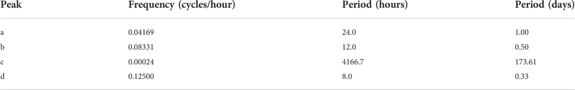
TABLE 3. Frequency and period characteristics of peaks on the ROTI periodogram.

Table 3 shows that the most prominent peak a) is associated with a period of 24 h, indicating that there is a strong diurnal signature on the ROTI data. The next most prominent peak b) is associated with a period of 12 h, indicating that there is also a semi-diurnal signature on the ROTI data. The next peak c) is associated with a period of ∼174 days (which is quasi semi-annual), indicating that there is also a seasonal signature on the ROTI data; 174/30 gives 5.8 (∼6) months variations. This depicts two major peaks. The solstice peaks are fairly low compared to the equinox peaks. The least of the four peaks d) is associated with a period of 8 h, indicating that there is also a weak terdiurnal signature on the ROTI data. The rest of the peaks are insignificant and therefore will not be considered for discussion. For instance, the peak between 0.15 and 0.2 is associated with a period of 6 hours. There may be some variation caused by the position of the Sun like the 2-day terminators, mid-day, and midnight, which we ignored because of their insignificance.

3.3 Association between the rate of change of total electron content index values and geomagnetic storms

We considered two sources of geomagnetic storms: the corotating interaction regions (CIRs) and coronal mass ejections (CMEs). CIR-driven storms create more problems to space-based assets, while CME-driven storms cause more problems to Earth-based electrical systems (Borovsky & Denton, 2006). CME-driven storms are brief, have denser plasma sheets, have stronger Dst perturbation, and sometimes have solar energetic particle (SEP) events, which can produce new radiation belts, great auroras, geomagnetically induced currents (GICs), and topside ionosphere equatorial bubbles (i.e., M-I coupling effects), while CIR-driven storms have longer durations, have hotter plasma sheets (thus stronger spacecraft charging), and produce higher fluxes of relativistic electrons. CIR-driven storms are more hazardous to the spacecraft, while CME storms are more damaging to Earth-based systems.

Table 4 shows the entire list of the geomagnetic storms, which were considered for the investigation in the year 2012. There were 56 in total. The dates and the times of occurrence of the storm events and the strengths of the geomagnetic storm indices are all indicated in the table.

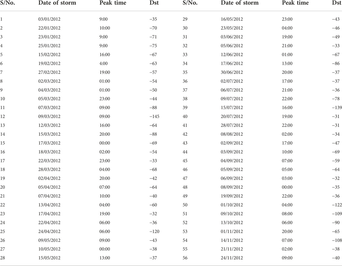
TABLE 4. Days of geomagnetic storm peaks in the year 2012, with Dst < −30 nT.

With this information in mind, all the storms were classified based on the intensity, the driver (CME or CIR). Figure 3 shows a summary of the classification in terms of strength of all geomagnetic storms of Dst ≤ −30 nT for the period between January 2012 and December 2012.

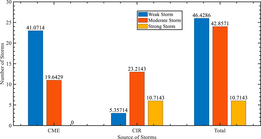
FIGURE 3. Graph of number of storms against storm sources, summarizing the storm classification in terms of strength of all Dst ≤ −30 nT for the period between January 2012 and December 2012. The numerical values on the tips of the bars represent the percentages over the overall number of storms.

During the study period, 46% of the storms were weak, 24% were moderate, and 11% were strong; 61% of the storms were CME-driven, while 39% of the storms were CIR-driven. The strong storms were all CIR-driven, while the bulk of the weak storm was CME-driven. Moderate storms were more or less equally CME- and CIR-driven.

The storms identified and tabulated in Table 4 were considered in the investigation. The seasonal pattern of irregularities is plotted in Figure 5. The data plotted were of the geomagnetic storms against ROTI. Out of the 56 storms identified in Table 4, 33 could have affected nighttime ionospheric irregularities, according to our investigations as evident by ROTI association.

The 33 geomagnetic storm events were further classified as per their sources. A total of 21 of the geomagnetic storms were found to be CME-driven, while 12 of the storms were CIR-driven. This is consistent with the results found by Matamba & Habarulema (2018) that during the solar maxima (e.g., in 2001 and 2012), mostly CME-driven storms were observed. It is known that CME- and CIR-driven storms generally occur during solar maximum and the declining phase of the solar cycle, respectively, (Matamba & Habarulema, 2018 and references therein), and the storms increase with an increase in solar activity and decrease with a decrease in solar activity.

The plots of Dst indices against ROTI on the day of storm are displayed in the subplots in Figure 4. Figure 4A represents the plot of all Dst values against the ROTI values, (b) represents the plots of the CIR-driven storms against the respective ROTI values, and (c) represents the plots of the CME-driven storms against the respective ROTI values.

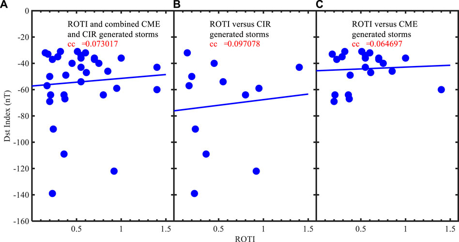
FIGURE 4. Plots of the minimum Dst against the ROTI values on the day of storm. The values, cc, on the plots represent the correlation coefficient of the parameters plotted. All the storm events were not associated with ionospheric disturbances. (A) Plot of all Dst values against the ROTI values; (B) plots of the CIR-driven storms against the respective ROTI values; and (C) plots of the CME-driven storms against the respective ROTI values.

The correlation coefficient between all the geomagnetic storm parameters and ROTI was obtained to be 0.073017, while those between all the CIR-driven geomagnetic storm parameters and the ROTI and CME-driven geomagnetic storm parameters and the ROTI were obtained to be 0.097078 and 0.064697, respectively. As much as the values were both low, the CIR-driven storms create more impact on the ionosphere, going by the correlation coefficient with the respective ROTI values.

3.4 Seasonal variation of ionospheric irregularities

The seasonal variation of the ionospheric irregularities over Abuja, Nigeria, is summarized in Figure 5. The four seasons in the years are named as March equinox (March and April), June solstice (May June, July, and August), September equinox (September and October), and December solstice (January, February, November, and December), according to classifications of seasons by Li et al. (2020).

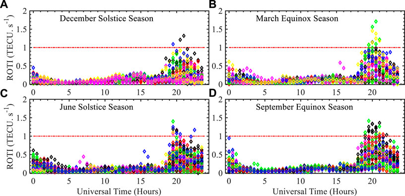
FIGURE 5. Seasonal variations of the times of occurrences of the ionospheric irregularities as determined using ROTI. The horizontal red lines are put arbitrarily to help in comparison of the trends across the seasons. Each color represents a satellite trace. (A) represents December solstice season, (B) represents the March equinox season, (C) represents the June solstice season and (D) represents the September equinox season.

The equinox months of September, October, March, and April were found to have the highest occurrences of ionospheric irregularities. The concentration of the data point above the 1 TEC/min mark was the highest during the equinox months and fairly sparse during the solstice months. The equinox months of March and April had majority of the irregularities occurring during the nighttime/early hours of the days, before sunrise. The peak time of occurrences of irregularities was 20:30 UT of the March equinox days. In the September and October equinoxes, the traces of maximum ionospheric irregularities occurred between 20:00 UT, approximately 30 min earlier than the time of peak irregularities for the March equinox. Day ionospheric irregularities as per our investigations were almost non-existent. The May, June, July, and August solstice months had more cases of irregularities with ROTI going beyond 1 TECU/min, followed the equinox months.

The irregularities would start at 18:00 UT except during the June solstice which would start at 18:30 UT and end at around 03:00 UT with minimal variations depending on the seasons.

3.5 Diurnal S4 index

Figure 6 shows the scintillation plots per satellite for the Ilorin (8.49664 and 4.54214) SCINDA GPS receiver for 13 April 2012. Out of the receiver stations listed in Table 2, only Ilorin had the data for this date. On the same date, there was a geomagnetic storm with minimum excursion and Dst index, −60 at 04:00 LT. The ROTI had a maximum index of 1.3 TECU·s⁻¹.

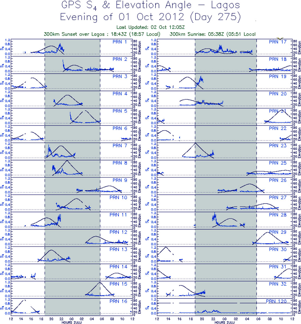
FIGURE 6. Scintillation plots per satellite for the Ilorin SCINDA GPS receiver for 13 April 2012.

The maximum S4 index recorded was about 1.0, mostly at around 22:00 LT, the reference satellites being PRN 14, 18, 21, and 22. According to Bhattacharyya et al. (2017), this was a strong scintillation. For any scintillation, S4 ≤ 0.2 is weak and S4 ≥ 1.0 is strong. This implies that 0.2 < S4 < 1.0 depicts a moderate scintillation.

Figure 7 shows the scintillation plots per satellite for the Lagos SCINDA GPS receiver, coordinates: 6.5166646 3.38499846, for 15 July 2012. On the same date, there was a strong geomagnetic storm at 16:00 LT of minimum Dst index, −139. The corresponding ROTI is 0.24 TECU·s⁻¹. From the S4 indices, as seen from the various satellite traces, the ionospheric irregularities were extremely low, despite the strong geomagnetic storm. Generally, the values of S4 indices for the entire month of July were low. Nsukka, Ile-Ife, Ilorin, and Akure SCINDA GPS receivers did not have their data archived.

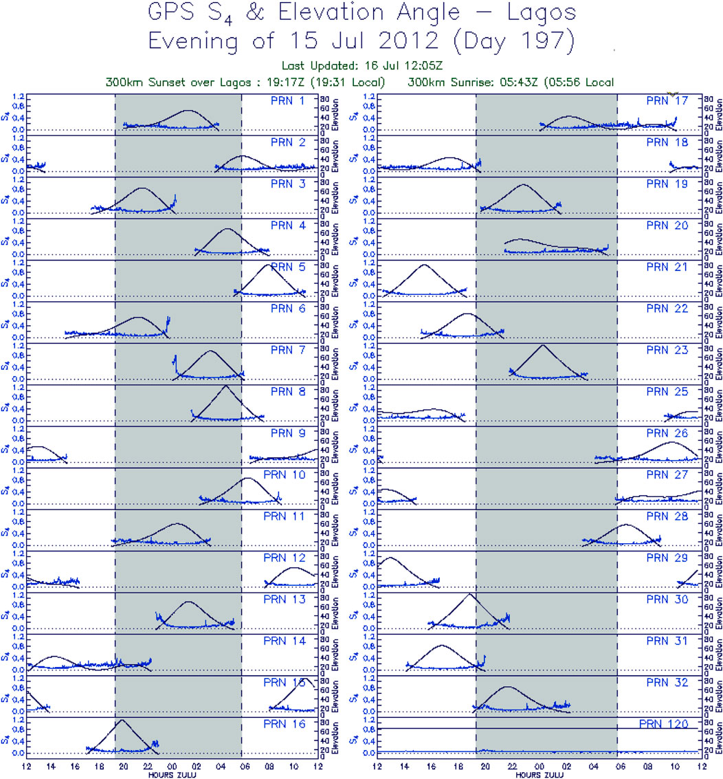
FIGURE 7. Scintillation plots per satellite for the Lagos SCINDA GPS receiver, with coordinates: 6.5166646 3.38499846, for 15 July 2012.

Next, Figure 8 shows the scintillation plots per satellite for the Lagos SCINDA GPS receiver, with coordinates: 6.5166646 3.38499846, for 1 October 2012. The geomagnetic storm index of the same date was the lowest at 04:00 LT and had the minimum Dst index of -122. The S4 indices could go as high as 0.6 during the night. This could be seen with the PRNs 1, 2, 5, 7, 8, 11, 17, 19, and 28, mostly at around 22:00 LT. The rest of the night generally remained quiet. The daytime irregularities remain negligible.

FIGURE 8. Scintillation plots per satellite for the Lagos SCINDA GPS receiver, with coordinates: 6.5166646 3.38499846, for 1 October 2012.

The data for 9 October 2012 were not available for all the receivers of the SCINDA GPS data.

The days of the geomagnetic occurrences were considered, and the estimate values of the S4 indices were noted. The observations did not bring any match between the magnitude of the geomagnetic storms and the S4 index. A sample of the observations is tabulated in Table 5. Apart from comparing with the Dst values, the date chosen for the tabulation cut across the four seasons of the year was compared as well. The magnitude of the S4 indices somehow followed the seasonal pattern with the highest values occurring during the equinoxes, in which the negligible values were observed during the solstices.

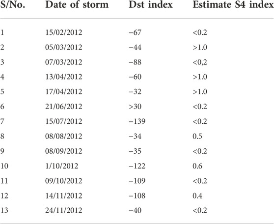
TABLE 5. Sampled dates of geomagnetic storm occurrences and corresponding estimate values of S4 indices.

4 Discussion

The first thing is that periods associated with the ROTI values were observed. The strong diurnal signature on the ROTI data observed in Figure 1A is attributed to the reason that the irregularities are mostly nighttime events, so there is an approximate 24-h period between typical fluctuations in ROTI. This is consistent with the results shown in the study proposed by Okoh et al. (2017). The study on the dependence of the occurrence rate on local time showed that the occurrence rate of plasma bubbles was higher during hours closer to the local midnight than during the later hours. The post-sunset irregularities were attributed to electrical processes in the evening time equatorial ionosphere. This is consistent with other studies which found that the formation of zonal wave-like structures over the broad longitude is the most reasonable phenomenon that is responsible for triggering the series of perturbations at the bottomside of the F-layer (Singh’ et al., 1997; Thampi et al., 2009; Tsunoda, 2011). At times, strong and weak perturbations could easily trigger EPBs through the RTI process during sunset hours, resulting from the rapid recombination at the bottomside of the F-layer. This shows that the seed perturbation and growth rate conditions are prerequisites for the development of the EPB.

The next most prominent peak is associated with a period of 12 h variation, as shown in Figure 1B. The least of the four peaks is associated with a period of 8 h, suggesting a weak terdiurnal signature on the ROTI data. We, however, considered that ROTI enhancement occurred between 19 and 24 LT so that the semi-diurnal and terdiurnal components are meaningless.

The peak for ∼174 days (which is quasi semi-annual), depicting a seasonal signature on the ROTI data observed in Figure 1C, depicted the seasonal variations of ionospheric irregularities. The two seasons are believed to be equinoxes and solstices. There are 4 months associated with equinoxes, and the rest of the months are associated with solstices. This is consistent with the finding by Buhari et al. (2017). In their work, they investigated that the seasonal variations of EPB occurrence recorded two minima during the solstice months every year. However, the occurrence rate during June–July was always higher than that during December–January and becomes more prominent in 2011–2013. They also asserted that most of the EPBs that occur during equinoctial months in 2011–2013 tend to occur successively along the observed longitudes.

The S4 indices also followed the seasonal variations rather than the influence of the geomagnetic storm occurrences. This was discovered by observing all the GIF plots of the S4 indices obtained from the SCINDA GPS data archive. The variations of the values of the S4 indices in the Nigerian SCINDA GPS receiver stations, namely, Lagos, Nsukka, Ile-Ife, Ilorin, and Akure, followed the seasonal patterns with the maximum values at the equinoxes and the minimum values at the solstice months. This is consistent with other researchers’ works, such as Bai et al. (2012), but a new finding in West Africa during the peak of SC 24. Kapil et al. (2022) also confirmed the temporal variation of the S4 index throughout the year 2014 at the Mumbai station. The scintillation occurrence is highly dependent on season, solar activity, and geographical locations. Other factors that can affect these irregularities are space weather conditions and induced ionospheric electric and magnetic fields.

Second, there were minimal morning and daytime irregularities. A similar scenario was reported by Kil et al. (2020) and Kil et al. (2019). In this work, some artificial seeding mechanisms might not be overruled just as it was in the case of Li et al. (2018). Ionospheric irregularity-driven fossils of the previous night are also another possibility of the daytime F-region irregularities. Under the background eastward electric field at daytime, the irregularity structures could be elevated to high altitudes together with the upward drift of ambient plasma. At higher altitudes, the daytime irregularities could have greater opportunity to be observed owing to the low photoionization (or refilling) rate (Huang et al., 2013). The EPBs at relatively low altitude would be refilled by the process of photochemical reaction. On the other hand, the ion vertical drift velocity inside the fossil bubbles could be essentially the same as the background vertical plasma drift. The fossil bubbles could be stably embedded in the background ionosphere. Thus, the daytime F-region irregularities could still maintain the large-scale vertical structures covering hundreds of kilometers in altitude (Xie et al., 2020).

As discussed previously, the daytime plume structures could be ionospheric plasma irregularity-driven fossils of the previous night that drift zonally toward the West African sector and particularly Abuja in Nigeria. Generally, the F-region plasma drifts are eastward at night and turn to westward near dawn as was the case in Fejer et al. (2013). The increased zonal electric field near sunset that occurred nearly in phase with the pre-reversal zonal electric field could have also triggered the irregularity development and could have caused an enhancement in the intensity of a developing PB event (G. Li et al., 2010).

Third, the storms available were also studied. Most of the storms in the year 2012 were weak. Particularly, 46.43% of the storms were weak, 42.86% were moderate in strength, and only 10.71%, translating to six storms, were strong. The 24th solar cycle was generally a year of weak solar activity. Table 1 attests to the weak geomagnetic activity, which shows similar trend as the weak solar activity. It is not easy to comment on the strength of the geomagnetic activities given that we are just considering 1 year. However, Echer et al. (2011) observed that there was an indication in their work that less-intense storms have their peak occurrences in the declining phase, while more-intense storms tend to have higher occurrence rates near solar maximum. It is therefore imperative that the entire year, 2012, had weak and moderate storms.

Fourth, there were observed irregularities predominantly at night. These are seen in Figures 2, 4 showing plots of ionospheric irregularities against times of the day. The nighttime irregularities are believed to be caused by the ionospheric plasma irregularities in the equatorial ionospheric F-region (Otsuka, 2018). They develop under the unique condition of the low inclination geomagnetic field lines that confine the F-region plasma to its low-latitude conjugate E-layers (Abdu, M. A., 2019).

During the main phase of geomagnetic storms, plasma bubbles at the evening terminator likely occur because the under-shielding prompt penetration electric field (PPEF) is superposed on pre-reversal enhancement (PRE) causing larger upward $E\times B$ drifts. The under-shielding penetration electric fields are driven by the solar wind-magnetosphere dynamo owing to the negative excursion of the north–south (Bz) component of the interplanetary magnetic field (IMF). The under-shielding prompt penetration electric field is directed eastward in the dayside and dusk sectors and westward in the night and dawn sectors.

During the recovery phase of geomagnetic storms, the plasma bubble occurrence at the evening terminator is suppressed, but plasma bubbles likely occur after midnight until dawn. The over-shielding penetration electric field, driven by the development of region-2 field-aligned currents, is directed westward in the dayside and dusk sectors and eastward in the night and dawn sectors. The disturbance dynamo electric field is also directed westward in the dayside and dusk sectors and eastward in the night and dawn sectors.

The irregularity growth in the F-region is possible only under the condition that the driving electric field cannot be shorted out by the E-layer conductivity, a condition that can exist after the day terminator. In the case of Nigeria, the local time is the universal time plus one (UTC+1), and 18:00 UT is therefore 19:00 LT, which essentially is the day terminator.

Fifth, it was evident that the geomagnetic storms were not absolutely responsible for technological impairment, which could be occasioned by ionospheric irregularities as measured by ROTI. There were minimal correlations between geomagnetic indices, Dst, and the irregularity parameters, ROTI, as is demonstrated in Figure 4, where the correlation coefficient was 0.073. It should be noted that not all geomagnetic storms would lead to enhancement of the ionospheric irregularities and scintillations. This is in line with the findings of Aarons (1991) that not all ionospheric irregularities are the result of the storms. It is of interest that the findings of Aarons (1991) and DasGupta et al. (1985) over 20 years ago using one methodology was confirmed using a more recent methodology of ROTI in our work. Aarons (1991) observed that if the maximum Dst occurred during the midnight-to-post-midnight time period, irregularities were driven. If the maximum Dst occurred in the early afternoon, irregularities were inhibited. If the maximum occurred around sunset or shortly after sunset, then there was no effect on the generation of irregularities that night.

Furthermore, the effect of geomagnetic storm on ionospheric irregularities could only be experienced after the day terminator. Abdu (1997), in their study of the major phenomena of the equatorial ionosphere–thermosphere system under disturbed conditions, observed that an increase in the evening trans-equatorial wind coupled with or otherwise and a decrease in the zonal wind arising from storm-induced disturbance thermospheric circulation could cause inhibition of equatorial spread F (ESF)/plasma bubble development. It is, however, necessary to determine the precise local time interval of a meridional wind enhancement that comes before an associated evening ESF/plasma bubble inhibition. It is also important to examine the associated equatorial ionospheric anomaly (EIA) symmetry/asymmetry conditions.

Late night occurrences (that is, not associated with sunset processes) of ESF and EIA can be initiated by the prompt penetration eastward electric field. However, no observation of their concurrent occurrences has so far been reported (Abdu, 1997).

Sixth, the statistical analysis of the seasonal variations indicated that the equinox months had the highest percentage occurrences of ionospheric irregularities in general. This is in line with the finding of Makela et al. (2004). They demonstrated a clear tendency for the occurrence of equatorial plasma bubbles at the Hawaiian longitudes during the near-equinoctial periods (mid-April until mid-May and mid-August until mid-October). It is during these periods that bubbles would often be seen immediately after sunset. June solstice followed the equinox months with the percentage occurrences of ionospheric irregularities. The least occurrences of irregularities were observed during the December solstice months. During the equinoxes, the Sun is by and large directly above the equator. The level of ionization of the ionosphere is higher and so the Es- and F-irregularities are more pronounced.

Finally, during the peak of the 24th solar cycle, and particularly, in 2012, there were more CME-driven geomagnetic storms than CIR-driven storms. This is in line with an established fact that CIR-driven storms generally occur in the late declining phase of the solar cycle and that CME-driven storms tend to occur at solar maximum (J. E. Borovsky & Denton, 2006; Matamba & Habarulema, 2018).

For both types of storms, the ion and electron temperatures are substantially elevated over typical values, probably because the solar wind speed is high and the plasma sheet temperature is related to the solar wind velocity (Borovsky, E. et al., 1998).

5 Conclusion

In this study, we have presented the results of the investigations to figure out the relationship between geomagnetic storm occurrence and ionospheric irregularity occurrence during the peak of the 24th solar cycle over the West African sector, and Nigeria in particular. The results give a better insight into how the geoeffectiveness of the solar events can affect the irregularity and scintillation occurrences and therefore the technology, which depend on the ionospheric conditions for their operations.

On the actual relationship between geomagnetic storms and the ionospheric irregularities, negligible correlations existed between the ROTI and the geomagnetic storms. The low values of correlation coefficients between the Dst and the parameters of the irregularities indicated that the irregularities do not depend only on the geomagnetic storms. There are other causes of ionospheric irregularities. Periods associated with the ROTI values as computed from the PSD of the input fluctuation vector were observed. The strong diurnal signature on the ROTI data indicated diurnal variation of the ROTI. There was also a semi-diurnal signature on the ROTI data. This repeated itself after every 12 h. The seasonal variation depicted by the ROTI and SCINDA GPS data was plotted to get the S4 indices that depicted the seasons of the year. There was no significant match between the magnitude of the geomagnetic storms and the S4 index. The magnitude of the S4 indices somehow followed the seasonal pattern with the highest values occurring during the equinoxes, in which the negligible values were observed during the solstices. We have equinoxes and solstices as the seasons of the year. We also saw a weak terdiurnal signature on the ROTI data.

Finally, during the descending peak phase of the 24th solar cycle, there were more CME-driven geomagnetic storms than CIR-driven storms. The majority of the storms, in the peak of the 24th solar cycle, are weak, followed by the number of moderate storms.

Data availability statement

The raw data supporting the conclusion of this article will be made available by the authors, without undue reservation.

Author contributions

All authors listed have made a substantial, direct, and intellectual contribution to the work and approved it for publication.

Acknowledgments

The authors appreciate the source of NIGNET GNSS data. They also appreciate the Air Force Research Laboratory for granting them access to the SCINDA GPS data. The authors also acknowledge the World Data Center (WDC) for geomagnetism, Kyoto, Japan, from whose website the geomagnetic data were obtained. The first author thanks the Scientific Committee on Solar-Terrestrial Physics (SCOSTEP) for presenting him the Visiting Scientist Award 2020, which helped the author carry out his work at the Space Environment Research Laboratory of the Centre for Atmospheric Research, Abuja. The authors thank the Centre for Atmospheric Research, National Space Research and Development Agency (CAR-NASRDA), Nigeria, for hosting, facilitating the research work, providing the financial and technical support, and providing all that were necessary for the research. The center continued supporting the work even long after the lapse of the award period. The authors also thank the Technical University of Kenya for supporting the research financially and providing other technical support.

Conflict of interest

The authors declare that the research was conducted in the absence of any commercial or financial relationships that could be construed as a potential conflict of interest.

Publisher’s note

All claims expressed in this article are solely those of the authors and do not necessarily represent those of their affiliated organizations, or those of the publisher, the editors, and the reviewers. Any product that may be evaluated in this article, or claim that may be made by its manufacturer, is not guaranteed or endorsed by the publisher.

References

Aarons, J. (1991). The role of the ring current in the generation or inhibition of equatorial F layer irregularities during magnetic storms. Radio Sci. 26 (4), 1131–1149. doi:10.1029/91RS00473
Abdu, M. A. (2019). Equatorial F region irregularities. Dyn. Ionos. A Syst. Approach Ionos. Irregularity 1, 169–178. doi:10.1016/B978-0-12-814782-5.00012-1
Abdu, M. A. (1997). Major phenomena of the equatorial ionosphere-thermosphere system under disturbed conditions. J. Atmos. Sol. Terr. Phys. 59 (13), 1505–1519. doi:10.1016/s1364-6826(96)00152-6
Badruddin, A., and Falak, Z. (2016). Study of the geoeffectiveness of coronal mass ejections, corotating interaction regions and their associated structures observed during Solar Cycle 23. Astrophys. Space Sci. 361 (8), 253–316. doi:10.1007/s10509-016-2839-4
Bai, W., Sun, Y., Xia, J., Tan, G., Cheng, C., Yang, G., et al. (2012). Global S4 index variations observed using FORMOSAT-3/COSMIC GPS RO technique during a solar minimum year. J. Geophys. Res. 117 (9), 1–31. doi:10.1029/2012JA017966
Basu, S., Groves, K. M., Quinn, J. M., and Doherty, P. (1999). A comparison of TEC fluctuations and scintillations at Ascension Island. J. Atmos. Solar-Terrestrial Phys. 61 (16), 1219–1226. doi:10.1016/S1364-6826(99)00052-8
Bhattacharyya, A., Kakad, B., Gurram, P., Sripathi, S., and Sunda, S. (2017). Development of intermediate-scale structure at different altitudes within an equatorial plasma bubble: Implications for L-band scintillations. J. Geophys. Res. Space Phys. 122 (1), 1015–1030. doi:10.1002/2016JA023478
Borovsky, E., Thomsen, F., Mccomas, D. J., Cayton, T. E., and Knipp, D. J. (1998). Magnetospheric dynamics and mass flow during the November 1993 storm. J. Geophys. Res. Space Phys. 103, 26373–26394. doi:10.1029/97JA03051
Borovsky, J. E., and Denton, M. H. (2006). Differences between CME-driven storms and CIR-driven storms. J. Geophys. Res. 111 (7), A07S08–17. doi:10.1029/2005JA011447
Buhari, S. M., Abdullah, M., Hasbi, A. M., Otsuka, Y., Yokoyama, T., Nishioka, M., et al. (2014). Continuous generation and two-dimensional structure of equatorial plasma bubbles observed by high-density GPS receivers in Southeast Asia. J. Geophys. Res. Space Phys. 119 (12), 10,569–10,580. doi:10.1002/2014JA020433
Buhari, S. M., Abdullah, M., Yokoyama, T., Otsuka, Y., Nishioka, M., Hasbi, A. M., et al. (2017). Climatology of successive equatorial plasma bubbles observed by GPS ROTI over Malaysia. J. Geophys. Res. Space Phys. 122 (2), 2174–2184. doi:10.1002/2016JA023202
Burch, J. L., Moore, T. E., Torbert, R. B., and Giles, B. L. (2016). Magnetospheric multiscale overview and science objectives. Space Sci. Rev. 199 (1–4), 5–21. doi:10.1007/s11214-015-0164-9
Campbell, W. H. (1979). Occurrence of AE and Dst geomagnetic index levels and the selection of the quietest days in a year. J. Geophys. Res. 84 (A3), 875. doi:10.1029/ja084ia03p00875
DasGupta, A., Maitra, A., and Das, S. K. (1985). Post-midnight equatorial scintillation activity in relation to geomagnetic disturbances. J. Atmos. Terr. Phys. 47 (8–10), 911–916. doi:10.1016/0021-9169(85)90067-4
Echer, E., Gonzalez, W. D., and Tsurutani, B. T. (2011). Statistical studies of geomagnetic storms with peak Dst≤-50nT from 1957 to 2008. J. Atmos. Solar-Terrestrial Phys. 73 (11–12), 1454–1459. doi:10.1016/j.jastp.2011.04.021
Fejer, B. G., Tracy, B. D., and Pfaff, R. F. (2013). Equatorial zonal plasma drifts measured by the C/NOFS satellite during the 2008-2011 solar minimum. JGR. Space Phys. 118 (6), 3891–3897. doi:10.1002/jgra.50382
Gopalswamy, N. (2009). Halo coronal mass ejections and geomagnetic storms. Earth Planets Space 61 (5), 595–597. doi:10.1186/BF03352930
Huang, C. S., De La Beaujardiere, O., Roddy, P. A., Hunton, D. E., Ballenthin, J. O., and Hairston, M. R. (2013). Long-lasting daytime equatorial plasma bubbles observed by the C/NOFS satellite. JGR. Space Phys. 118 (5), 2398–2408. doi:10.1002/jgra.50252
Hughes, W. J. (2009). Space weather: Physics and effects. Trans. Am. Geophys. Union 90 (9). doi:10.1029/2009eo090010
Kapil, C., Seemala, G. K., Shetti, D. J., and Acharya, R. (2022). Reckoning ionospheric scintillation S4 from ROTI over Indian region. Adv. Space Res. 69 (2), 915–925. doi:10.1016/j.asr.2021.10.026
Kendall, P. C., Chapman, S., Akasofu, S. I., and Swartztrauber, P. N. (1966). The computation of the magnetic field of any axisymmetric current distribution—With magnetospheric applications. Geophys. J. Int. 11 (3), 349–364. doi:10.1111/j.1365-246X.1966.tb03088.x
Kil, H., Lee, W. K., and Paxton, L. J. (2020). Origin and distribution of daytime electron density irregularities in the low-latitude F region. J. Geophys. Res. Space Phys. 125 (9), e2020JA028343. doi:10.1029/2020JA028343
Kil, H., Paxton, L. J., Lee, W. K., and Jee, G. (2019). Daytime evolution of equatorial plasma bubbles observed by the first Republic of China satellite. Geophys. Res. Lett. 46 (10), 5021–5027. doi:10.1029/2019GL082903
Li, G., Ning, B., Abdu, M. A., Wang, C., Otsuka, Y., Wan, W., et al. (2018). Daytime F-region irregularity triggered by rocket-induced ionospheric hole over low latitude. Prog. Earth Planet. Sci. 5 (1), 11. doi:10.1186/s40645-018-0172-y
Li, G., Ning, B., Hu, L., Liu, L., Yue, X., Wan, W., et al. (2010). Early intensive insulin therapy in newly diagnosed type 2 diabetes: The size of the problem. Zhonghua Nei Ke Za Zhi 115 (4), 1–2. doi:10.1029/2009JA014830
Li, Q., Zhu, Y., Fang, K., and Fang, J. (2020). Statistical study of the seasonal variations in tec depletion and the roti during 2013–2019 over Hong Kong. Sensors Switz. 20 (21), 6200–6217. doi:10.3390/s20216200
Ma, G., and Maruyama, T. (2006). A super bubble detected by dense GPS network at east Asian longitudes. Geophys. Res. Lett. 33 (21), L21103–L21105. doi:10.1029/2006GL027512
Makela, J. J., Ledvina, B. M., Kelley, M. C., and Kintner, P. M. (2004). Analysis of the seasonal variations of equatorial plasma bubble occurrence observed from Haleakala, Hawaii. Ann. Geophys. 22 (9), 3109–3121. doi:10.5194/angeo-22-3109-2004
Matamba, T. M., and Habarulema, J. B. (2018). Ionospheric responses to CME- and CIR-driven geomagnetic storms along 30°e–40°E over the african sector from 2001 to 2015. Space weather. 16 (5), 538–556. doi:10.1029/2017SW001754
Mendillo, M., Lin, B., and Aarons, J. (2000). The application of GPS observations to equatorial aeronomy. Radio Sci. 35 (3), 885–904. doi:10.1029/1999RS002208
Miller, E. S., Makela, J. J., and Kelley, M. C. (2009). Seeding of equatorial plasma depletions by polarization electric fields from middle latitudes: Experimental evidence. Geophys. Res. Lett. 36 (18), 1–5. doi:10.1029/2009GL039695
Nishioka, M., Saito, A., and Tsugawa, T. (2008). Occurrence characteristics of plasma bubble derived from global ground-based GPS receiver networks. J. Geophys. Res. 113 (5), 1–12. doi:10.1029/2007JA012605
Okoh, D., Rabiu, B., Shiokawa, K., Otsuka, Y., Segun, B., Falayi, E., et al. (2017). First study on the occurrence frequency of equatorial plasma bubbles over west Africa using an all-sky airglow imager and GNSS receivers. J. Geophys. Res. Space Phys. 122 (12), 12430–12444. doi:10.1002/2017JA024602
Oladipo, O. A., and Schüler, T. (2013). Equatorial ionospheric irregularities using GPS TEC derived index. J. Atmos. Solar-Terrestrial Phys. 92, 78–82. doi:10.1016/j.jastp.2012.09.019
Otsuka, Y. (2018). Review of the generation mechanisms of post-midnight irregularities in the equatorial and low-latitude ionosphere. Prog. Earth Planet. Sci. 5 (1), 57. doi:10.1186/s40645-018-0212-7
Perreault, P., and Akasofu, S. I. (1978). A study of geomagnetic storms. Geophys. J. Int. 54 (3), 547–573. doi:10.1111/j.1365-246X.1978.tb05494.x
Pi, X., Mannucci, A. J., Lindqwister, U. J., and Ho, C. M. (1997). Monitoring of global ionospheric irregularities using the worldwide GPS network. Geophys. Res. Lett. 24 (18), 2283–2286. doi:10.1029/97GL02273
Rama Rao, P. V. S., Gopi Krishna, S., Vara Prasad, J., Prasad, S. N. V. S., Prasad, D. S. V. V. D., and Niranjan, K. (2009). Geomagnetic storm effects on GPS based navigation. Ann. Geophys. 27 (5), 2101–2110. doi:10.5194/angeo-27-2101-2009
Richardson, I. G., and Cane, H. V. (2011). Galactic cosmic ray intensity response to interplanetary coronal mass ejections/magnetic clouds in 1995 - 2009. Sol. Phys. 270 (2), 609–627. doi:10.1007/s11207-011-9774-x
Seemala, G. K., and Valladares, C. E. (2011). Statistics of total electron content depletions observed over the South American continent for the year 2008. Radio Sci. 46 (5). doi:10.1029/2011RS004722
Singh’, S., Johnson, F. S., and Power, R. A. (1997). Gravity wave seeding of equatorial plasma bubbles. J. Geophys. Res. 102 (4), 7399–7410. doi:10.1029/96JA03998
Thampi, S. V., Yamamoto, M., Tsunoda, R. T., Otsuka, Y., Tsugawa, T., Uemoto, J., et al. (2009). First observations of large-scale wave structure and equatorial spread F using CERTO radio beacon on the C/NOFS satellite. Space Sci. 36 (18). doi:10.1029/2009GL039887
Tsunoda, R. T. (2011). Performance analysis of OFDM modulation on indoor broadband PLC channels. EURASIP J. Adv. Signal Process 78. doi:10.1186/s40645-015-0038-5
Veronig, A. M., Jain, S., Podladchikova, T., Pötzi, W., and Clette, F. (2021). Hemispheric sunspot numbers 1874 – 2020. Astrophysics 56, 1–12. doi:10.1051/0004-6361/202141195
Xie, H., Yang, S., Zhao, X., Hu, L., Sun, W., Wu, Z., et al. (2020). Unexpected high occurrence of daytime F-region backscatter plume structures over low latitude Sanya and their possible origin. Geophys. Res. Lett. 47 (22), 0–3. doi:10.1029/2020GL090517
Yang, Z., and Liu, Z. (2016). Correlation between ROTI and ionospheric scintillation indices using Hong Kong low-latitude GPS data. GPS Solut. 20 (4), 815–824. doi:10.1007/s10291-015-0492-y
Keywords: scintillation, ROTI, geomagnetic storms, CME, CIR, equatorial ionosphere, ionospheric irregularities
Citation: Ondede GO, Rabiu AB, Okoh D, Baki P, Olwendo J, Shiokawa K and Otsuka Y (2022) Relationship between geomagnetic storms and occurrence of ionospheric irregularities in the west sector of Africa during the peak of the 24th solar cycle. Front. Astron. Space Sci. 9:969235. doi: 10.3389/fspas.2022.969235
Received: 14 June 2022; Accepted: 31 October 2022;
Published: 17 November 2022.
Edited by:
Andrés Calabia, Polytechnic University of Madrid, SpainReviewed by:
Jiandong Liu, UMR8539 Laboratoire de Météorologie Dynamique (LMD), FranceTeshome Dugassa, Space Science and Geospatial Institute, Ethiopia
Copyright © 2022 Ondede, Rabiu, Okoh, Baki, Olwendo, Shiokawa and Otsuka. This is an open-access article distributed under the terms of the Creative Commons Attribution License (CC BY). The use, distribution or reproduction in other forums is permitted, provided the original author(s) and the copyright owner(s) are credited and that the original publication in this journal is cited, in accordance with accepted academic practice. No use, distribution or reproduction is permitted which does not comply with these terms.
*Correspondence: George Ochieng Ondede, georgeochieng08@gmail.com