Whistler turbulence vs. whistler anisotropy instability: Particle-in-cell simulation and statistical analysis

1 Introduction

High-frequency short-wavelength whistler turbulences are often observed in space plasma (Beinroth and Neubauer, 1981; Lengyel-Frey et al., 1996; Narita et al., 2011, 2016). We define whistler turbulence as a broadband ensemble of incoherent field fluctuations in a magnetized plasma at frequencies between the lower hybrid and electron cyclotron frequencies and at wavelengths much shorter than the ion inertial length. There have been significant debates about the possible sources of whistler turbulence in recent years. One possible scenario is the cascade of fluctuations from the longer wavelength inertial range. Kinetic Alfvén waves and higher frequency magnetosonic-whistler fluctuations have been considered as the two candidates (Gary and Smith, 2009). Recent solar wind observations (Leamon et al., 1998; Sahraoui et al., 2009, 2010; Kiyani et al., 2012; Salem et al., 2012) and numerical simulations (Howes et al., 2008; TenBarge et al., 2013) have identified the existence of the kinetic Alfvén fluctuations with a wavelength around the ion inertial length or ion thermal gyro-radius. However, the mechanism on how such modes cascade fluctuation energy down to electron scale remains unclear. For instance, as the inertial range cascade preferentially transfers fluctuation energy to propagation directions relatively perpendicular to background magnetic field, where whistler fluctuations can be damped (Mithaiwala et al., 2012; Cerri et al., 2016), the cascade processes may not be able to provide a sufficiently large amplitude to feed to whistler turbulence.

Another possible scenario is kinetic whistler instabilities. A specific growing mode which can be a source for whistler turbulence at relatively long electron-scale wavelengths is the whistler anisotropy instability. We use subscripts “⊥″ and “‖″ to denote the directions perpendicular and parallel to the background magnetic field B₀, respectively, subscripts e and i to denote electrons and ions, respectively, and $\vec{k}$ to denote the wave-vector. This instability is driven by electron temperature anisotropy T_⊥e/T_‖e > 1 and propagates at $\vec{k}\times {\mathit{B}}_0=0$ in a homogeneous plasma. Observations have indicated that this instability is operating in the terrestrial magnetosheath (Gary et al., 2005). In the solar wind, while adiabatic expansion of the solar wind would typically lead to T_‖e > T_⊥e which can excite the firehose instability, there is evidence that local compressions and turbulence in the solar wind may also create T_⊥e > T_‖e (Gary and Madland, 1985; Gary, 1993; Karimabadi et al., 2013), which can excite the whistler instability. Particle-in-Cell (PIC) simulations (Gary and Wang, 1996; Gary et al., 2000, 2014; Saito et al., 2008) have demonstrated that this mode can generate enhanced whistler fluctuations and spectral transfer (Gary and Wang, 1996; Gary et al., 2000, 2014; Saito et al., 2008; Chang et al., 2014, 2015).

To further investigate the aforementioned scenarios, one must first understand the competing effects from whistler turbulence and whistler anisotropy instability. For instance, one of the primary consequences of plasma turbulence is to produce sharp spatial gradients in the plasma which can produce enhanced anisotropies locally and forward cascade to dissipate the energy from long wavelength to short wavelength (Osman et al., 2010; Greco et al., 2012; Parashar and Matthaeus, 2016). On the other hand, simulations of whistler anisotropy instabilities driven by a bi-Maxwellian velocity distribution for electrons in a homogeneous plasma showed that the instability imposes an upper bound or constraint on that anisotropy uniformly across the plasma (Gary and Wang, 1996; Gary et al., 2000, 2014; Hughes et al., 2016). The electron anisotropy upper bound derived by Gary and Wang (1996) was verified by observations in the solar wind and magnetosphere (Gary et al., 2005; MacDonald et al., 2008; Štverák et al., 2008; An et al., 2017). However, past studies have mostly addressed the effects from whistler turbulence and whistler anisotropy instability separately.

Gary et al. (2008, 2010), Saito et al. (2008, 2010), and Saito and Gary (2012) presented the first 2-dimensional (2D) PIC simulations of whistler turbulence, and Gary et al. (2012, 2014) and Chang et al. (2011, 2013, 2014, 2015) presented the first 3-dimensional (3D) PIC simulations of whistler turbulence. These simulations considered a homogeneous, magnetized, collisionless plasma upon which an initial spectrum of relatively long wavelength whistler fluctuations is imposed. The results showed that the forward cascade leads to fluctuations which are consistent with the linear dispersion solution for whistler fluctuations. Electron temperature anisotropy were also found to form during forward cascade. Hughes et al. (2014, 2017) and Gary et al. (2016) further investigated electron/ion heating due to whistler turbulence as a function of the initial fluctuating magnetic field energy density, and found the maximum electron heat rate scales approximately linearly with the fluctuating field energy density. This suggests a quasi-linear type heating due to electron Landau damping (Gary et al., 2016).

In this paper, we consider a collisionless, magnetized plasma with co-existing whistler turbulence and the electron temperature anisotropy as the initial condition, and investigate the consequences of both microinstability growth and turbulent cascade using 3D fully kinetic PIC simulations. Qudsi et al. (2020) and Bandyopadhyay et al. (2020) carried out 2D PIC simulations of the Alfvénic turbulence, where ion temperature anisotropy is generated by the development of the turbulence. The results showed that microinstabilities can develop locally in response to ion temperature anisotropies generated by turbulence and may affect the plasma globally, and that there is an apparent correlation between linear instability theory and strongly intermittent turbulence. It was also speculated that a similar process might also occur on electron scale. In this paper, in order to evaluate the effect from whistler instability at a given temperature anisotropy, we prescribe electron temperature anisotropy as the initial condition to drive the instability.

We carry out four different ensembles of PIC simulations: 1) an initially quiet, anisotropic plasma with prescribed initial electron temperature anisotropy; 2) an isotropic plasma with prescribed initial whistler fluctuations; 3) an anisotropic plasma with initial whistler fluctuations (varying initial electron temperature anisotropy and fixed initial fluctuation field energy); and 4) an anisotropic plasma with initial whistler fluctuations (fixed initial electron temperature anisotropy and varying initial fluctuation field energy). Results from PIC simulation are linked with a statistical analysis to understand whether there is any interplay between whistler turbulence and whistler instability, and what are the competing effects from these two processes.

2 Simulation model and setup

We consider a collisionless electron-ion plasma with a uniform background magnetic field ${\mathit{B}}_0=B_0\widehat{z}$. For the jth (j = e, i) species, we denote the plasma frequency as ${\omega }_{pj}=\sqrt{4\pi n_j{e}^2/m_j}$, the cyclotron frequency as Ω_j = eB₀/m_jc, the thermal speed as $v_{tj}=\sqrt{T_{\Vert j}/m_j}$, and ${\beta }_j=8\pi n_j{T}_{\Vert j}/B_0^2$. We denote the angle of mode propagation θ by k ⋅B₀ = kB₀ cos(θ).

The physical and numerical parameters are chosen to assure that the consequences of both microinstability growth and turbulent cascade can be accurately resolved in the simulation. In this paper, the initial electron plasma beta is taken to be of a typical value for the solar wind plasma, β_e = 0.1. To study the effects of whistler anisotropy instability, we consider a range of initial T_⊥e/T_‖e values that are below and above the instability threshold in the simulation. Through a sequence of test runs with varying initial T_⊥e/T_‖e values, we find the threshold to excite whistler anisotropy instability for the parameters considered is T_⊥e/T_‖e ≃ 2.3, close to the calculation using the linear theory from (Gary, 1993). In this paper, we present simulations with initial temperature anisotropy of T_⊥e/T_‖e = 1, 2, 3, 5, 7, 9. To study the effects of whistler turbulence, an ensemble of whistler fluctuations are imposed at t = 0. The initially loaded whistler fluctuations are set to be relatively long-wavelength with approximately isotropic wavevectors. The spectrum is the same as that used in our previous simulation studies on whistler turbulence (Chang et al., 2011; Gary et al., 2012; Chang et al., 2013; Hughes et al., 2014; Chang et al., 2015). The initial whistler modes include n = 0, ±1, ±2, and ±3 of the fundamental wavenumber in the perpendicular direction, and n = ±1, ±2, and ±3 of the fundamental wavenumber in the parallel direction, where the fundamental wavenumber corresponds to the maximum wavelength that can be contained in the domain. This leads to a total of N = 150 normal modes with random phases (Chang et al., 2013). The simulations will consider initial total fluctuating magnetic field energy density.

at ϵ = 0, 0.05, 0.25, and 0.5.

We apply a three-dimensional (3D) full particle electromagnetic particle-in-cell code, 3D-EMPIC by Wang et al. (1995), to simulate the evolution of plasma under four different sets of initial conditions. In Simulation Group A, the ions are set to follow an isotropic velocity distribution while the electrons follow an anisotropic bi-Maxwellian velocity distribution function with different initial values of T_⊥e/T_‖e, at T_⊥e/T_‖e = 2, 3, 5, 7, and 9. The plasma has no initial field fluctuations, ϵ = 0. Simulation Group A is a typical setup for simulations of whistler anisotropy instability (Gary and Wang, 1996). In Simulation Group B, both the ions and electrons are set to have an isotropic velocity distribution. An ensemble of whistler fluctuations are imposed at t = 0, with the initial total fluctuating magnetic field energy density at ϵ = 0, 0.05, 0.25, and 0.5. The initial condition in Simulation Groups C and D is a combination of that of Groups A and B, where the electrons follow an anisotropic bi-Maxwellian velocity distribution function and the plasma is initially loaded with an ensemble of whistler fluctuations. In Group C, we take the initial field fluctuation at ϵ = 0.25 and change the initial temperature anisotropy at T_⊥e/T_‖e = 2, 3, 5, 7, 9. In Group D, we take the initial temperature anisotropy at T_⊥e/T_‖e = 3 and change the initial field fluctuation field density at ϵ = 0, 0.05, 0.25, 0.50. The simulation groups are summarized in Table 1.

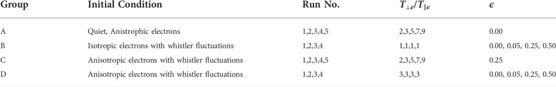
TABLE 1. Summary of simulation cases. In all cases, β_e = 0.1 and v_te/c = 0.1.

All the simulations are run using an artificial ion to electron mass ratio of m_i/m_e = 400. The ion initial temperature is set to be T_i = T_‖e. The ratio of the electron gyro-frequency to plasma frequency is Ω_e/ω_pe ≃ 0.447. The simulation box is a cube with a size in each direction at 51.2d_e, where d_e = c/ω_e is the electron inertial length. The grid spacing is set to be Δ = 0.10d_e, and hence the mesh size is 512 × 512 × 512. The time step is set to be Δtω_pe = 0.05. All the simulations are run for tω_pe > 1000 (tΩ_pe > 447.20), i.e. more than 20,000 steps. The macro-particles used is 48 ions and 48 electrons per cell or about 3.1 × 10¹¹ total macro-particles.

We use the Probability Density Function (PDF) in statistical analysis of magnetic fluctuations. The PDF of a random field B(x) may be defined as (Matthaeus et al., 2015)

Then the increments of the field components are

where r is the spatial separation length vector along the direction of any unit vector e_r. By summing over all the cells of a PIC simulation, one may construct a PDF for each component of the fluctuating fields as a function of the spatial separation r. If the random variable r is subject to a central limit theorem, the distribution is expected to be a Gaussian, whereas any departure from a Gaussian corresponds to a more strongly intermittent ensemble of fluctuations. An important advantage of the PDF analyses is that, by statistically averaging over a large body of observational and/or computational data, one may draw general conclusions which are less readily available via other means of data analysis. For example, the statistical analysis of solar wind magnetic fluctuations measured from the Cluster and ACE spacecraft by Kiyani et al. (2012) shows that the PDFs of both δB_‖ and δB_⊥ exhibit the same functional form in the kinetic range but not in the inertial range. The PDF analysis of the solar wind data from the Helios spacecraft (He et al., 2013) shows that, as the heliospheric distance of the spacecraft increases, the distribution of the local mean magnetic field vectors gradually broadens in the radial direction and becomes more scattered. The PDF analysis of 3D PIC simulations of whistler turbulence (Chang et al., 2014) shows distinct non-Gaussian “tails” in both the δB_‖ and δB_⊥ distributions as well as distinctly different functional forms between the two magnetic polarizations.

3 Results and discussions

3.1 Fluctuating magnetic fields

Figure 1 shows the normalized fluctuating magnetic field energy density averaged over all mesh points, $|\delta B(t){|}^2/B_0^2$, as a function of time for all the simulation runs. The results from Group A show that the fluctuating magnetic fields in Run A2 through A5 (T_⊥e/T_‖e ≥ 3) grow rapidly to saturation, with the growth rate in the linear phase matching the value calculated from the linear theory (Gary, 1993). This is similar to that in previous simulations of whistler anisotropy instability (Gary and Wang, 1996), where it showed pitch-angle scattering of the electrons by fluctuating magnetic fields reduces T_⊥e and increases T_‖e, and thus the temperature anisotropy. In Run A1 (T_⊥e/T_‖e = 2), the fluctuating magnetic field stays relatively unchanged because the initial anisotropy is below the instability excitation threshold and thus the instability is not excited. The results from Group B show that the fluctuating magnetic field energy decreases with time. This is similar to that in previous simulations of whistler turbulence (Gary et al., 2012), where it showed that the decrease of fluctuating magnetic field corresponds to an increase in the electron thermal energy with the parallel electron temperatures gaining more energy than the perpendicular electron temperatures. Gary et al. (2012) showed that such energy dissipation is primarily through wave-particle interactions via linear Landau damping at relatively small initial fluctuating field energy (0.02 ≤ ϵ ≤ 0.2) and fully nonlinear processes at large initial fluctuating field energy (ϵ > 0.2). Recent studies have suggested that both nonlinear Landau damping (Ganguli et al., 2010; Chang et al., 2013; Li et al., 2016) and current structure dissipation (Wan et al., 2012, 2015; Karimabadi et al., 2013) contribute to the nonlinear dissipation processes. Chang et al. (2014) suggested current structure dissipation as the dominant nonlinear dissipation process in whistler turbulence.

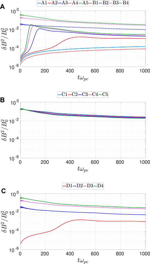
FIGURE 1. Time history of $\delta B{(t)}^2/B_0^2$ for all simulation cases. (A) Simulation Groups A and B (B) Simulation Group C (C) Simulation Group D

The results from Group C show that, for a plasma with co-existing whistler fluctuations and electron temperature anisotropy as the initial condition, the time history of $|\delta B(t){|}^2/B_0^2$ is almost identical to that from Run B3 (ϵ = 0.25, T_⊥e/T_‖e = 1). The initial temperature anisotropy, whether below the instability threshold (Run C1) or above the instability threshold (Run C2 through C5), has little effect on $|\delta B{(t)}^2|/B_0^2$. Comparing the results from Group D with that from Group B further shows that the time history of $|\delta B(t){|}^2/B_0^2$ is influenced only by the initial fluctuating field energy density ϵ. The whistler anisotropy instability has almost no effect on the evolution of the overall magnitude of the fluctuating magnetic fields.Figure 2 shows the magnetic fluctuation wavevector anisotropy averaged over all mesh points

as a function of time for all the simulation runs. The tan²θ_B history in Run A1 is nearly constant as no whistler anisotropy instability is excited. The results from Run A2 through A5 follow the predictions of the linear theory (Gary, 1993): the maximum growth rate happens in the direction of k ×B = 0; the energy in the perpendicular direction is quickly damped due to resonance scattering of pitch angle, and thus the energy perturbation is mostly along B₀. The results from Group B shows that the wavevector anisotropy increases rapidly. Larger initial fluctuating magnetic field energy density leads to a more rapid increase in wavevector anisotropy. This reflects the effect of forward cascade of whistler turbulence, which transfers the energy preferentially for k_⊥≫ k_‖, thus leading to the expansion of wavevector in the perpendicular direction. The forward cascade of whistler turbulence was discussed in detail in Gary et al. (2012) and Chang et al. (2011, 2013, 2014).

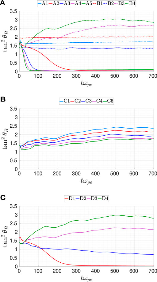
FIGURE 2. Time history of tan²θ_B for all simulation cases. (A) Simulation Groups A and (B) Simulation Group C (C) Simulation Group D

The tan²θ_B history from Group C qualitatively follows that of Run B3 (ϵ = 0.25, T_⊥e/T_‖e = 1). However, the initial temperature anisotropy also has a limited effect, showing that an increase of T_⊥e/T_‖e reduces the growth rate of tan²θ_B. This may be explained as a result of the action by the whistler anisotropy instability. A larger initial temperature anisotropy leads to a larger growth rate of whistler anisotropy instability, which in turn leads to stronger scattering of pitch angle, and thus faster damping of the energy in the perpendicular direction. Comparing the results from Group D with that from Group B, we find that, at a given initial temperature anisotropy, the effect of the whistler instability diminishes as the initial fluctuating field energy increases. This suggests that forward cascade from whistler turbulence has a far more dominating effect over pitch angle scattering from whistler instability on wavevector anisotropy.

To further investigate the effects of the whistler anisotropy instability on the intermittency generated by whistler turbulence, we calculate the probability density function (PDF) of the local fluctuating magnetic δB (i, j, k) for each cell. Figure 3 shows the PDF along the y direction. For Groups A and C, the PDFs from Run A1 and C1 are not shown because the whistler anisotropy instability is not excited in these two cases. Figure 3E (Run B1) shows the result for a quiet isotropic plasma. Figures 3A–D (Run A2-A5 from Group A) show the result for a quiet anisotropic plasma. The initial temperature anisotropy excites whistler anisotropy instability. As there is little change in the tail region, the whistler anisotropy instability did not generate enhanced whistler fluctuations for the simulation parameters considered. Figures 3E–H (Group B) show the result for an isotropic plasma with whistler fluctuations. Similar to previous simulations of whistler turbulence (Chang et al., 2014), an increase in ϵ leads to an enhanced tail region and the increased deviation from the Gaussian distribution. Figures 3I-L (Group C) show the PDFs for Group C are qualitatively similar to that in Group B, indicating that increasing the initial electron temperature anisotropy has very little effect on the fluctuating magnetic fields. Figures 3M–P (Group D) further show that the PDFs are only influenced by the initial fluctuating field energy. The results from Figures 1–3 are not surprising. As the magnetic field energy from the broad band whistler turbulence dominates over that from the narrow band, the operation of whistler anisotropy instability will have a very minor effect on the evolution of the fluctuating magnetic field.

FIGURE 3. Comparison of the probability distribution function of δB_‖ along Y axis at Ω_et ≈ 111.80. (A)–(D): Run A2 to A5. (E)–(H): Run B1 to B4. (I)–(L): Run C2 to C5 (M)–(P): Run D1 to D4.

3.2 Electron temperature anisotropy

We next compare the effects of whistler turbulence and whistler instability on electron temperature anisotropy. We calculate both the local temperature anisotropy R_e (i, j, k) = T_⊥e (i, j, k)/T_‖e (i, j, k) from macro-particles in each cell and the average temperature anisotropy over all the cells of the simulation domain

where N_x, N_y, N_z are the total mesh points each direction, and subscripts i, j, k denote the cell number. Figure 4 compares R_e vs. β_e for Groups A and C at ω_pet = 1000 (Ω_et ≃ 447.2), when both the whistler turbulence and the whistler instability are developed (see Figure 1).

FIGURE 4. Average electron temperature anisotropy R_e v. s. β_e at Ω_et = 0 and at Ω_et ≈ 447.2 for Group A and Group C. The initial anisotropies are shown as transparent circle for Group A and transparent square for Group C, respectively. The final anisotropies for Run A1 through A5 are color circles with increasingly dark shades, and that for Run C1 through C5 are color squares with increasingly dark shades. The upper bound predicted by Eq. 6 is shown as the dotted line.

Gary and Wang (1996) showed that the wave-particle scattering from whistler instability imposes an upper bound on T_⊥e/T_‖e commensurate with that predicted by linear theory:

where S_e is the dimensionless scalar conductivity of electrons (Gary, 1993; Gary and Wang, 1996). The anisotropy upper bound in the form of Eq. 6 was numerically fitted in Gary and Wang (1996) for parameters similar to that used here, and is shown as the dotted line in Figure 4. The results show that the average temperature anisotropy R_e at the end of the simulations from Run A2 through A5 lay under the upper bound of Eq. 6. The R_e from Run A1 is almost unchanged, as expected, as the whistler instability is not excited in this case. It is interesting to observe that the R_e points from Group C are further below the upper bound from the linear theory prediction.

As turbulence produces strong inhomogeneity in plasma, we next examine the contours of local electron temperature anisotropy, R_e (i, j, k). Figures 5, 6 show the contours of R_e (i, j, k), on an x-y plane in the middle of the simulation domain, where we compare R_e (i, j, k) for increasing initial fluctuating field energy (from left to right) for a fixed initial temperature anisotropy (T_⊥e/T_‖e = 3). In Figure 6, we compare R_e (i, j. k) for increasing initial T_⊥e/T_‖e (from left to right) for a fixed initial fluctuating field energy (ϵ = 0.25). Both Figures 5, 6 are plotted for ω_pet = 500 (Ω_et ≃ 223.6), when all the cases are starting to approach an asymptote.

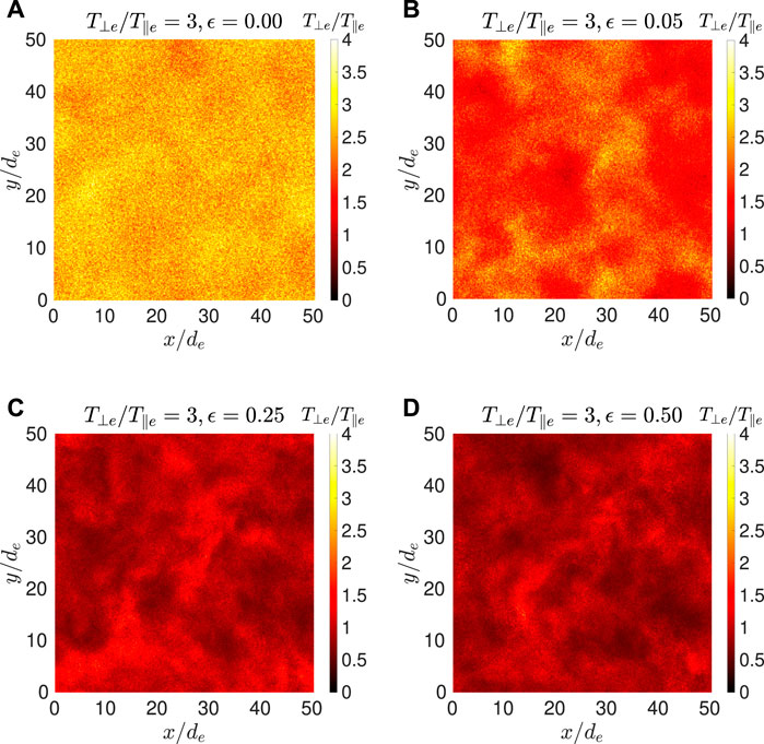
FIGURE 5. Contours of R_e (i, j, k) on an x-y plane in the middle of the simulation box at time Ω_et ≈ 223.60 for Run D1 (A), D2 (B), D3 (C), and D4 (D).

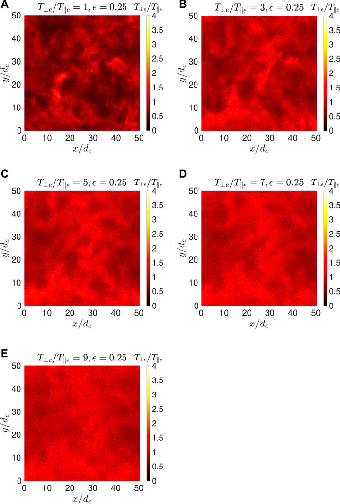
FIGURE 6. Contours of R_e (i, j, k) on an x-y plane in the middle of the simulation box at time Ω_et ≈ 223.60 for Run B3 (A), C2 (B), C3 (C), C4 (D), and C5 (E).

Figure 5A (Run D1) has no initial whistler fluctuation and thus the temperature anisotropy distribution is homogenous. As the initial spectrum strength ϵ increases, Figure 5 shows increasing intermittent fluctuations in temperature anisotropy due to turbulence. Figure 6A (Run B3) shows that turbulence produces strong anisotropies in an initially isotropic plasma. All of these results are to be expected. However, in Figure 6, as the initial anisotropy increases, we find that the intermittent fluctuations in the R_e (i, j, k) contours start to diminish. The range of R_e (i, j, k) in Figure 6 (from left to right) is summarized in Table 2, showing the temperature becomes more homogenous as the initial T_⊥e/T_‖e increases.

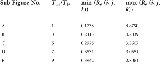
TABLE 2. R_e (i, j, k) value range of Figure 6.

Figures 5, 6 show that, in contrast to the minor effects on the fluctuating magnetic field, the whistler anisotropy instability has a major effect on the intermittency of temperature anisotropy generated by turbulence. The whistler anisotropy instability acts to reduce electron temperature anisotropy through wave-particle scattering. Wave-particle scattering is a microscopic process. Wave-particle scattering of electrons are affected more efficiently by local field fluctuations and are less dependent on the overall field energy. The results suggest that the fluctuation from the growth of a single mode of whistler anisotropy instability is more efficient in wave-particle scattering of the electrons than that of a spectrum of whistler modes. A stronger initial temperature anisotropy leads to a larger whistler instability growth rate, and stronger wave-particle scattering effect, and thus reducing the intermittency in temperature anisotropy generated by turbulence.

4 Summary and conclusion

3D PIC simulations are carried out to study the dynamic evolution of a collisionless, magnetized plasma with co-existing whistler turbulence and electron temperature anisotropy as the initial condition, and the competing consequences of whistler turbulence cascade and whistler anisotropy instability growth. The results show that the operation of the whistler instability within whistler turbulence has no obvious effects on the fluctuating magnetic field. We find the overall fluctuating magnetic field energy and intermittency generated by turbulence are not influenced by the inclusion of an initial electron temperature anisotropy, while wavevector anisotropy is reduced somewhat by increased electron temperature anisotropy. In contrast, the results show that whistler instability has a major effect on electron temperature anisotropy. While whistler turbulence produces sharp gradients and enhanced electron temperature anisotropies locally, we find that increasing the initial electron temperature anisotropy actually leads to a reduction of the intermittency in the electron temperature anisotropy generated by turbulence, and the reduction of the average electron temperature anisotropy further below the upper bound as predicted by the linear theory for a homogeneous anisotropic plasma. The results suggest the small reduction of wavevector anisotropy and major reduction of electron temperature anisotropy are apparently due to whistler instability growth. Comparing to an isotropic plasma with whistler turbulence, an increase in the initial electron temperature anisotropy leads to a larger growth rate of the whistler anisotropy instability, resulting in faster damping of the energy in this perpendicular direction, and thus a small reduction of the growth rate of the wavevector anisotropy tan²θ_B. While turbulence produce sharp gradients and local enhanced anisotropies, the whistler anisotropy instability acts to reduce electron temperature anisotropy through wave-particle scattering. The results suggest that the fluctuation from the growth of a single mode of whistler anisotropy instability is more efficient in wave-particle scattering of the electrons than that of a spectrum of whistler modes. Thus, a larger initial global electron temperature anisotropy, when combined with enhanced local electron temperature anistropy, would lead to even stronger wave-particle scattering effects locally, thus leading to local temperature anisotropy reduction and a more homogeneous electron temperature landscape.

In conclusion, we find that the overall effect of whistler anisotropy instability on a plasma with co-existing whistler turbulence and global electron temperature anisotropy is minor comparing to that of whistler turbulence. This is because the fluctuating energy associated with the narrowband whistler instability is dominated by that from the broadband whistler turbulence. However, as field fluctuations from the growth of a single instability mode may be more efficient in the wave-particle scattering process than that from a spectrum of whistler modes, the whistler instability can significantly reduces the intermittency of electron temperature anisotropy generated by turbulence. This suggests that microinstability may act as a regulation mechanism on turbulence development. In this study, the whistler instability is generated by imposing a bi-Maxwellian electron velocity distribution as the initial condition. The competing consequences of whistler turbulence cascade and whistler anisotropy instability growth will need to be further evaluated in a more realistic setup where the instability develops naturally from turbulence in future study.

Data availability statement

The raw data supporting the conclusions of this article will be made available by the authors, without undue reservation.

Author contributions

The authors contributed equally to this research.

Funding

SPG acknowledges support from NASA grant NNX16AM98G (80NSSC19K0652) and NSF Award 2031024. CC and JW acknowledge support from NSF Award 2031024 through a sub-award from Space Science Institute to USC.

Acknowledgments

CC and JW acknowledge helpful discussions with Vadim Roytershtey and the computational resources provided by the Cheyenne cluster (Computational And Information Systems Laboratory, 2017) at the National Center for Atmospheric Research (NCAR) and the computational resources provided by the Center for Advanced Research Computing at the University of Southern California (USC CARC).

Conflict of interest

The authors declare that the research was conducted in the absence of any commercial or financial relationships that could be construed as a potential conflict of interest.

Publisher’s note

All claims expressed in this article are solely those of the authors and do not necessarily represent those of their affiliated organizations, or those of the publisher, the editors and the reviewers. Any product that may be evaluated in this article, or claim that may be made by its manufacturer, is not guaranteed or endorsed by the publisher.

References

An, X., Yue, C., Bortnik, J., Decyk, V., Li, W., and Thorne, R. M. (2017). On the parameter dependence of the whistler anisotropy instability. JGR. Space Phys. 122, 2001–2009. doi:10.1002/2017ja023895
Bandyopadhyay, R., Qudsi, R. A., Matthaeus, W. H., Parashar, T. N., Maruca, B. A., Gary, S. P., et al. (2020). Interplay of turbulence and proton-microinstability growth in space plasmas. arXiv preprint arXiv:2006.10316.
Beinroth, H., and Neubauer, F. (1981). Properties of whistler mode waves between 0.3 and 1.0 au from helios observations. J. Geophys. Res. 86, 7755–7760. doi:10.1029/ja086ia09p07755
Cerri, S. S., Califano, F., Jenko, F., Told, D., and Rincon, F. (2016). Subproton-scale cascades in solar wind turbulence: Driven hybrid-kinetic simulations. Astrophys. J. 822, L12. doi:10.3847/2041-8205/822/1/l12
Chang, O., Gary, S. P., and Wang, J. (2013). Whistler turbulence at variable electron beta: Three-dimensional particle-in-cell simulations. J. Geophys. Res. Space Phys. 118, 2824–2833. doi:10.1002/jgra.50365
Chang, O., Gary, S. P., and Wang, J. (2015). Whistler turbulence forward cascade versus inverse cascade: Three-dimensional particle-in-cell simulations. Astrophys. J. 800, 87. doi:10.1088/0004-637x/800/2/87
Chang, O., Peter Gary, S., and Wang, J. (2014). Energy dissipation by whistler turbulence: Three-dimensional particle-in-cell simulations. Phys. Plasmas 21, 052305. doi:10.1063/1.4875728
Chang, O., Peter Gary, S., and Wang, J. (2011). Whistler turbulence forward cascade: Three-dimensional particle-in-cell simulations. Geophys. Res. Lett. 38. doi:10.1029/2011gl049827
Computational And Information Systems Laboratory (2017). Cheyenne: SGI ICE XA cluster. doi:10.5065/D6RX99HX
Ganguli, G., Rudakov, L., Scales, W., Wang, J., and Mithaiwala, M. (2010). Three dimensional character of whistler turbulence. Phys. Plasmas 17, 052310. doi:10.1063/1.3420245
Gary, S. P., Chang, O., and Wang, J. (2012). Forward cascade of whistler turbulence: Three-dimensional particle-in-cell simulations. Astrophys. J. 755, 142. doi:10.1088/0004-637x/755/2/142
Gary, S. P., Hughes, R. S., Wang, J., and Chang, O. (2014). Whistler anisotropy instability: Spectral transfer in a three-dimensional particle-in-cell simulation. J. Geophys. Res. Space Phys. 119, 1429–1434. doi:10.1002/2013ja019618
Gary, S. P., Hughes, R. S., and Wang, J. (2016). Whistler turbulence heating of electrons and ions: Three-dimensional particle-in-cell simulations. Astrophys. J. 816, 102. doi:10.3847/0004-637x/816/2/102
Gary, S. P., Lavraud, B., Thomsen, M. F., Lefebvre, B., and Schwartz, S. J. (2005). Electron anisotropy constraint in the magnetosheath: Cluster observations. Geophys. Res. Lett. 32, L13109. doi:10.1029/2005gl023234
Gary, S. P., and Madland, C. D. (1985). Electromagnetic electron temperature anisotropy instabilities. J. Geophys. Res. 90, 7607–7610. doi:10.1029/ja090ia08p07607
Gary, S. P., Saito, S., and Li, H. (2008). Cascade of whistler turbulence: Particle-in-cell simulations. Geophys. Res. Lett. 35, L02104. doi:10.1029/2007gl032327
Gary, S. P., Saito, S., and Narita, Y. (2010). Whistler turbulence wavevector anisotropies: Particle-in-cell simulations. Astrophys. J. 716, 1332–1335. doi:10.1088/0004-637x/716/2/1332
Gary, S. P., and Smith, C. W. (2009). Short-wavelength turbulence in the solar wind: Linear theory of whistler and kinetic alfvén fluctuations. J. Geophys. Res. 114. doi:10.1029/2009ja014525
Gary, S. P. (1993). Theory of space plasma microinstabilities. Cambridge atmospheric and space science series. Cambridge University Press. doi:10.1017/CBO9780511551512
Gary, S. P., and Wang, J. (1996). Whistler instability: Electron anisotropy upper bound. J. Geophys. Res. 101, 10749–10754. doi:10.1029/96ja00323
Gary, S. P., Winske, D., and Hesse, M. (2000). Electron temperature anisotropy instabilities: Computer simulations. J. Geophys. Res. 105, 10751–10759. doi:10.1029/1999ja000322
Greco, A., Valentini, F., Servidio, S., and Matthaeus, W. H. (2012). Inhomogeneous kinetic effects related to intermittent magnetic discontinuities. Phys. Rev. E 86, 066405. doi:10.1103/PhysRevE.86.066405
He, J., Tu, C., Marsch, E., Bourouaine, S., and Pei, Z. (2013). Radial evolution of the wavevector anisotropy of solar wind turbulence between 0.3 and 1 au. Astrophys. J. 773, 72. doi:10.1088/0004-637x/773/1/72
Howes, G., Dorland, W., Cowley, S., Hammett, G., Quataert, E., Schekochihin, A., et al. (2008). Kinetic simulations of magnetized turbulence in astrophysical plasmas. Phys. Rev. Lett. 100, 065004. doi:10.1103/physrevlett.100.065004
Hughes, R. S., Gary, S. P., and Wang, J. (2014). Electron and ion heating by whistler turbulence: Three-dimensional particle-in-cell simulations. Geophys. Res. Lett. 41, 8681–8687. doi:10.1002/2014gl062070
Hughes, R. S., Gary, S. P., and Wang, J. (2017). Particle-in-cell simulations of electron and ion dissipation by whistler turbulence: Variations with electron β. Astrophys. J. 835, L15. doi:10.3847/2041-8213/835/1/l15
Hughes, R. S., Wang, J., Decyk, V. K., and Gary, S. P. (2016). Effects of variations in electron thermal velocity on the whistler anisotropy instability: Particle-in-cell simulations. Phys. Plasmas 23, 042106. doi:10.1063/1.4945748
Karimabadi, H., Roytershteyn, V., Wan, M., Matthaeus, W., Daughton, W., Wu, P., et al. (2013). Coherent structures, intermittent turbulence, and dissipation in high-temperature plasmas. Phys. Plasmas 20, 012303. doi:10.1063/1.4773205
Kiyani, K. H., Chapman, S. C., Sahraoui, F., Hnat, B., Fauvarque, O., and Khotyaintsev, Y. V. (2012). Enhanced magnetic compressibility and isotropic scale invariance at sub-ion larmor scales in solar wind turbulence. Astrophys. J. 763, 10. doi:10.1088/0004-637x/763/1/10
Leamon, R. J., Smith, C. W., Ness, N. F., Matthaeus, W. H., and Wong, H. K. (1998). Observational constraints on the dynamics of the interplanetary magnetic field dissipation range. J. Geophys. Res. 103, 4775–4787. doi:10.1029/97ja03394
Lengyel-Frey, D., Hess, R., MacDowall, R., Stone, R., Lin, N., Balogh, A., et al. (1996). Ulysses observations of whistler waves at interplanetary shocks and in the solar wind. J. Geophys. Res. 101, 27555–27564. doi:10.1029/96ja00548
Li, T. C., Howes, G. G., Klein, K. G., and TenBarge, J. M. (2016). Energy dissipation and landau damping in two-and three-dimensional plasma turbulence. Astrophys. J. 832, L24. doi:10.3847/2041-8205/832/2/l24
MacDonald, E., Denton, M., Thomsen, M., and Gary, S. (2008). Superposed epoch analysis of a whistler instability criterion at geosynchronous orbit during geomagnetic storms. J. Atmos. solar-terrestrial Phys. 70, 1789–1796. doi:10.1016/j.jastp.2008.03.021
Matthaeus, W. H., Wan, M., Servidio, S., Greco, A., Osman, K. T., Oughton, S., et al. (2015). Intermittency, nonlinear dynamics and dissipation in the solar wind and astrophysical plasmas. Phil. Trans. R. Soc. A 373, 20140154. doi:10.1098/rsta.2014.0154
Mithaiwala, M., Rudakov, L., Crabtree, C., and Ganguli, G. (2012). Co-existence of whistler waves with kinetic alfven wave turbulence for the high-beta solar wind plasma. Phys. Plasmas 19, 102902. doi:10.1063/1.4757638
Narita, Y., Gary, S., Saito, S., Glassmeier, K.-H., and Motschmann, U. (2011). Dispersion relation analysis of solar wind turbulence. Geophys. Res. Lett. 38. doi:10.1029/2010gl046588
Narita, Y., Nakamura, R., Baumjohann, W., Glassmeier, K.-H., Motschmann, U., Giles, B., et al. (2016). On electron-scale whistler turbulence in the solar wind. Astrophys. J. 827, L8. doi:10.3847/2041-8205/827/1/l8
Osman, K., Matthaeus, W., Greco, A., and Servidio, S. (2010). Evidence for inhomogeneous heating in the solar wind. Astrophys. J. 727, L11. doi:10.1088/2041-8205/727/1/l11
Parashar, T. N., and Matthaeus, W. H. (2016). Propinquity of current and vortex structures: Effects on collisionless plasma heating. Astrophys. J. 832, 57. doi:10.3847/0004-637x/832/1/57
Qudsi, R. A., Bandyopadhyay, R., Maruca, B. A., Parashar, T. N., Matthaeus, W. H., Chasapis, A., et al. (2020). Intermittency and ion temperature–anisotropy instabilities: Simulation and magnetosheath observation. Astrophys. J. 895, 83. doi:10.3847/1538-4357/ab89ad
Sahraoui, F., Goldstein, M. L., Belmont, G., Canu, P., and Rezeau, L. (2010). Three dimensional AnisotropickSpectra of turbulence at subproton scales in the solar wind. Phys. Rev. Lett. 105, 131101. doi:10.1103/physrevlett.105.131101
Sahraoui, F., Goldstein, M., Robert, P., and Khotyaintsev, Y. V. (2009). Evidence of a cascade and dissipation of solar-wind turbulence at the electron gyroscale. Phys. Rev. Lett. 102, 231102. doi:10.1103/physrevlett.102.231102
Saito, S., and Gary, S. (2012). Beta dependence of electron heating in decaying whistler turbulence: Particle-in-cell simulations. Phys. Plasmas 19, 012312. doi:10.1063/1.3676155
Saito, S., Gary, S. P., Li, H., and Narita, Y. (2008). Whistler turbulence: Particle-in-cell simulations. Phys. Plasmas 15, 102305. doi:10.1063/1.2997339
Saito, S., Gary, S. P., and Narita, Y. (2010). Wavenumber spectrum of whistler turbulence: Particle-in-cell simulation. Phys. Plasmas 17, 122316. doi:10.1063/1.3526602
Salem, C. S., Howes, G., Sundkvist, D., Bale, S., Chaston, C., Chen, C., et al. (2012). Identification of kinetic alfvén wave turbulence in the solar wind. Astrophys. J. 745, L9. doi:10.1088/2041-8205/745/1/l9
Štverák, Š., Trávníček, P., Maksimovic, M., Marsch, E., Fazakerley, A. N., and Scime, E. E. (2008). Electron temperature anisotropy constraints in the solar wind. J. Geophys. Res. 113. doi:10.1029/2007ja012733
TenBarge, J., Howes, G., and Dorland, W. (2013). Collisionless damping at electron scales in solar wind turbulence. Astrophys. J. 774, 139. doi:10.1088/0004-637x/774/2/139
Wan, M., Matthaeus, W., Karimabadi, H., Roytershteyn, V., Shay, M., Wu, P., et al. (2012). Intermittent dissipation at kinetic scales in collisionless plasma turbulence. Phys. Rev. Lett. 109, 195001. doi:10.1103/physrevlett.109.195001
Wan, M., Matthaeus, W., Roytershteyn, V., Karimabadi, H., Parashar, T., Wu, P., et al. (2015). Intermittent dissipation and heating in 3d kinetic plasma turbulence. Phys. Rev. Lett. 114, 175002. doi:10.1103/physrevlett.114.175002r
Keywords: whistler anisotropy instability, whistler turbulence, space plasma, 3D fully kinetic EMPIC simulation, statistical analysis
Citation: Cui C, Gary SP and Wang J (2022) Whistler turbulence vs. whistler anisotropy instability: Particle-in-cell simulation and statistical analysis. Front. Astron. Space Sci. 9:941241. doi: 10.3389/fspas.2022.941241
Received: 11 May 2022; Accepted: 25 July 2022;
Published: 19 August 2022.
Edited by:
Misa Cowee, Los Alamos National Laboratory (DOE), United StatesReviewed by:
Yasuhito Narita, Austrian Academy of Sciences (OeAW), AustriaMuhammad Fraz Bashir, University of California, Los Angeles, United States
Copyright © 2022 Cui , Gary and Wang. This is an open-access article distributed under the terms of the Creative Commons Attribution License (CC BY). The use, distribution or reproduction in other forums is permitted, provided the original author(s) and the copyright owner(s) are credited and that the original publication in this journal is cited, in accordance with accepted academic practice. No use, distribution or reproduction is permitted which does not comply with these terms.
*Correspondence: Joseph Wang, josephjw@usc.edu