Ion alfvén velocity fluctuations and implications for the diffusion of streaming cosmic rays

1 Introduction

Magnetized turbulence is the rule and not the exception for the dynamics of the interstellar medium (ISM) in star-forming galaxies. Turbulence is a high-Reynolds-number (Re > 10³) fluid state, where the Reynolds number is defined as Re = (σ_VL)/ν, and σ_V is the velocity dispersion on length scale L with kinematic viscosity ν. Most astrophysical systems are vastly larger than the scales that are important for viscosity, and hence, turbulence has spread across most scales in the galaxies, with typical star-forming, cold molecular clouds boasting Re ∼ 10⁹ (Krumholz, 2015). Due to the turbulent dynamo (e.g., Schekochihin et al., 2004; Federrath, 2016; Xu and Lazarian, 2016; McKee et al., 2020; Seta and Federrath, 2021a; Xu and Lazarian, 2021b), the energy in magnetic fields of the ISM is roughly at equipartition with the turbulent kinetic energy (Boulares and Cox, 1990; Zweibel and McKee, 1995; Beck and Wielebinski, 2013; Seta and Beck, 2019). Magnetic fields play a dynamical role in the ISM, acting as a scaffold for the gas density through large-scale flux-freezing, facilitating some of the rich structure that we observe, e.g., in ISM observations (Li and Henning, 2011; Li et al., 2013; Soler et al., 2013; Ade et al., 2016; Aghanim et al., 2016; Cox et al., 2016; Federrath et al., 2016; Malinen et al., 2016; Tritsis and Tassis, 2016; Soler et al., 2017; Tritsis et al., 2018; Heyer et al., 2020; Pillai et al., 2020), and simulations of ISM turbulence (Soler and Hennebelle, 2017; Tritsis et al., 2018; Beattie and Federrath, 2020; Körtgen and Soler, 2020; Seifried et al., 2020; Barreto-Mota et al., 2021). The ISM is also energy dense in relativistic, charged particles–cosmic rays.

1.1 Cosmic Rays and the Streaming Instability

Cosmic rays (CRs) are high-energy (non-thermal), charged particles, that spiral around magnetic field lines at a radius set by the balance between Lorentz and centrifugal forces. Averaged over the ISM in star-forming galaxies, the energy densities of CRs, turbulent motions, and magnetic fields are roughly in equipartition (Boulares and Cox, 1990; Beck and Wielebinski, 2013; Seta and Beck, 2019). CRs are important for understanding the ionization (hence chemistry) and thus heating of interstellar gas (Field et al., 1969; Xu and Yan, 2013; Krumholz et al., 2020), and in turn influence the evolution of galaxies. For example, CR pressure gradients can significantly impact the morphology of simulated, ideal galaxies (Salem et al., 2014) and can drive and sustain galactic winds (and more general outflows) with mass-loading factors of order unity, which in turn can excite turbulent gas motions (Uhlig et al., 2012; Booth et al., 2013; Girichidis et al., 2016; Crocker et al., 2021a; b). Because these processes depend upon CR pressure gradients, transport of CRs through the ISM is important to understand.

If magnetic fields in the ISM were static and structureless on scales of the CR gyroradius, CR transport would be trivial–CRs would simply spiral along field lines, moving down them at the speed of light times the cosine of the pitch angle between the CR velocity vector the local magnetic field. However, Alfvén waves with frequencies comparable to the frequency of CR gyration can resonantly scatter CRs, randomly changing their pitch angle. Moreover, when a population of CRs is numerous enough, they themselves can excite such scattering waves via the streaming instability (Lerche, 1967; Kulsrud and Pearce, 1969; Wentzel, 1969; Skilling, 1971). CRs that have an energy range between ∼ GeV − TeV, which dominate the CR pressure budget (Evoli, 2018), are likely to excite waves so efficiently that to zeroth order the CRs are scattered isotropically in pitch angle around field lines, still traveling at relativistic velocities. However, to first order, a slight asymmetry in the scattering distribution develops such that there is a bulk velocity along the field, v_stream, that approaches the ion Alfvén speed, $v_{\text{A,ion}}=B/\sqrt{4\pi \chi \rho }$, where B is the magnitude of the local magnetic field, ρ is the gas density and χ is the ionization fraction by mass. The asymmetry corresponds to an advective process whereby the population of scattering cosmic rays move down CR pressure gradients and along the field lines (Caprioli et al., 2009; Bell, 2013; Krumholz et al., 2020; Xu and Lazarian, 2021a; Bustard and Zweibel, 2021; Sampson et al., 2022). Throughout this study, we will refer to CRs that have self-confined to stream at close to v_A,ion as SCRs (streaming cosmic rays).

As we have described, the streaming instability is an advective process, e.g., the small asymmetry in the scattering angle distribution leads to the population of SCRs being advected down pressure gradients, along field lines. However, consider now multiple populations of SCRs distributed across a plasma and that we are “observing” on length scales larger than the correlation length scale ¹ of the magnetic field embedded in the medium, ${\ell }_{\text{cor}}/{\ell }_0\sim {\mathcal{M}}_{\text{A}}^{-2}$, where ${\mathcal{M}}_{\text{A}}={\sigma }_V/v_{\text{A}}$ is the Alfvén Mach number, assuming a supersonic, Burgers velocity dispersion - size relation, ${\sigma }_v(\ell /{\ell }_0)\sim {(\ell /{\ell }_0)}^{1/2}$ (Federrath et al., 2021). On these scales, the field is tangled, chaotic (at least for ${\mathcal{M}}_{\text{A}}\gtrsim 2$, Beattie et al., 2020), and different regions in space have causally disconnected magnetic fields. For average ISM parameters, ${\mathcal{M}}_{\text{A}}\approx 2$ (Gaensler et al., 2011; Krumholz et al., 2020; Seta and Federrath, 2021a; Liu et al., 2021), ℓ₀ ∼ 100 pc (∼ the Galactic disk scale-height; Karlsson et al., 2013; Falceta-Gonçalves et al., 2014; Li et al., 2014; Krumholz and Ting, 2018), then on scales beyond ℓ_cor ∼ 25 pc streaming cosmic rays, locked to magnetic field lines, take tangled, chaotic paths that resemble a random walk, leading to a spatial dispersion between cosmic rays originating from the same source. We call this process the “macroscopic diffusion” of SCRs.

However, it is not only tangling of magnetic field lines above the correlation length that may be responsible for creating spatial dispersion between populations of SCRs. Because SCRs become self-confined to travel at $v_{\text{A,ion}}\propto B/\sqrt{\chi \rho }$ inhomogeneities in ionic Alfvén wave speeds may arise in either the magnetic field or the gas density and contribute to the macroscopic diffusion of SCRs. Gas density fluctuations can occur on scales much smaller than the correlation scale of the magnetic field (e.g., ion fluctuations down to less than AU scales, Armstrong et al., 1995). A detailed experimental study of diffusion for streaming cosmic rays is beyond the scope of this study, and is presented with great detail in Sampson et al. (2022). In this study we explore the ionic Alfvén wave fluctuations in a compressible, magnetized turbulent medium across a broad range of plasma parameters describing the diffuse, warm atomic medium to dense (possibly sub-Alfvénic–Li et al., 2013; Federrath et al., 2016; Hu et al., 2019; Heyer et al., 2020; Hwang et al., 2021; Hoang et al., 2021; Skalidis et al., 2021b) highly-supersonic molecular clouds, highlighting the role of compressibility in the generation of the inhomogeneities in ionic Alfvén wave speeds. To the authors’ knowledge, these fluctuations have not been studied in the astrophysical compressible turbulence literature, even though Alfvén waves, and the speed in which they travel, have deep roots in MHD turbulence theory and phenomenology (e.g., Elsasser, 1950; Iroshnikov, 1964; Kraichnan, 1965; Sridhar and Goldreich, 1994; Goldreich and Sridhar, 1995; Boldyrev, 2006). However, the ingredients for developing a theory for understanding the variance of ionic Alfvén velocities, and more broadly their 1-point volume-weighted PDF, have been developed. These are, of course, the density and magnetic field fluctuations. Turbulence theory is a collection of two-point statistical models; however in this study, we explore and develop 2^nd moment theories, which are more easily applied to observations of interstellar gas. Before progressing to the results of this study we consider three theoretical aspects of the problem: 1) what is the state of the ionization by mass in typical ISM conditions? and what is the nature of 2) the density and 3) the magnetic field fluctuations, up to 2^nd moments, in compressible MHD turbulence? We start with the first.

1.2 On the Ionization State of Turbulent Density Fluctuations

We first consider the ionization fraction χ, for the purposes of demonstrating why we need not account for its fluctuations separately. In equilibrium in a region with a constant ionization rate per neutral particle ζ, the condition for equilibrium is simply balance between the ionization and recombination rates per unit volume,

where n_n, n_e, and n_ion are the number densities of neutral species, electrons, and ions, respectively and α_rec is the recombination rate coefficient for free electrons with ions. For simplicity consider a region of weakly ionized plasma, χ ≪ 1, where all ions are singly ionized. In this case we have n_ion = n_e = χρ/μ_ionm_H, where μ_ion is the mean atomic mass of ions and m_H is the hydrogen mass. Similarly, we have n_n = ρ/μm_H, where μ is the mean atomic mass of neutrals, and therefore

Thus in equilibrium we should expect χ ∝ ρ^−1/2.

However, since we are interested in fluctuations, we must next ask whether equilibrium is an appropriate assumption. The timescale required for a given parcel of gas to reach ionization equilibrium is the ion density divided by the rate at which the ion density changes,

Significantly, this does not depend on the density, except indirectly through χ. We can therefore immediately determine characteristic values of t_ion for different phases of the ISM. In the atomic ISM, we generally expect to have χ ∼ 10^–3 − 10^–1, μ = 1.4 (for the standard cosmic mix of H and He), μ_ion = 1 (H is the dominant ionized species), and ζ ∼ 10^–16 s⁻¹ (Wolfire et al., 2003), and therefore t_ion ∼ 0.4–40 Myr; in the interior of a molecular cloud, the equilibrium ionization fraction is lower, χ ∼ 10^–6, and we have μ = 2.33 (H₂ + He composition), μ_i = 29 (HCO⁺ is the dominant charge carrier–Krumholz et al., 2020), and ζ ∼ 10^–16 − 10^–17 s⁻¹, and t_ion ∼ 30–300 y.

This should be compared to the characteristic timescale over which the density changes which, for a turbulent medium, Scannapieco and Safarzadeh (2018) show is given approximately by

where τ is the flow crossing time, s = ln (ρ/ρ₀) is the logarithmic over-density in a region with mean density ρ₀, and s_∗ is a constant of order unity that depends on the Mach number and Alfvén Mach number of the flow. This timescale varies from τ/3 to zero slowly as a function of s.

The above allows a few immediate conclusions. In the molecular ISM, we can safely assume instantaneous equilibrium: molecular clouds have flow crossing times of $\sim 1$ Myr, compared to times of at most a few hundred years to reach ionization equilibrium. Even in the colder parts of the atomic ISM, which tend to have χ ∼ 10^–3, instantaneous equilibrium is probably a safe assumption, since characteristic crossing times of the atomic ISM are of order 10 Myr, while at χ ∼ 10^–3 we have t_ion ≲ 1 Myr. Only in the diffuse atomic ISM are we likely to encounter regions where the ionization equilibration time is comparable to or longer than the flow crossing timescale. For this reason, we will simply assume a relationship χ ∝ ρ^−1/p, for any p in what follows. Clearly, p → ∞ (χ ∼constant), corresponds to the diffuse atomic ISM, and p = 2 for the other phases, which are in ionization equilibrium. Reality should lie between these two limiting cases. Having established the ionization state of the density fluctuations, we now turn our attention to the spatial statistics of the density fluctuations themselves in the lognormal framework.

1.3 Lognormal Density Fluctuation Theory

One of the key differences between incompressible and compressible turbulence is the dynamical role of density fluctuations and shocked gas in the turbulent plasma. Lognormal models for the PDF of turbulent ρ/ρ₀ fluctuations first originate from Vazquez-Semadeni (1994). Vazquez-Semadeni considers a linear density fluctuation in a self-similar (scale-free), isothermal plasma, where thermal pressure, $(1/{\mathcal{M}}^2)\nabla c_s^2\rho$, is negligible $(\mathcal{M}\gg 1)$, where $\mathcal{M}={\sigma }_v/c_s$ is the sonic Mach number, and the gas is not bounded by self-gravity, α_vir ∝ E_kinetic/|E_grav|≫ 1, where E_kinetic is the kinetic and |E_grav| is the gravitational energy, respectively. With these assumptions in hand, the lognormal PDF is motivated by assuming that for time, t_n, a density fluctuation can be expressed as a multiplicative interaction through density fluctuations at previous times,

where ρ(t₀)/ρ₀ = ρ₀/ρ₀ = 1 is the initial density, before the turbulent interactions, in units of the mean. Under the log-transformation, the density fluctuations become additive,

turning the problem into one that involves the sum of random variables. If each ρ(t_n)/ρ₀ ∀n, is generated by the same underlying distribution and is statistically independent from each of the other fluctuations, ${⟨s(t_n)s(t_m)⟩}_t=\delta (t_n-t_m)$, i.e., each addition of an extra fluctuation to Eq. 5 does not depend upon the current state of ρ(t_n)/ρ₀), then ρ(t_n)/ρ₀ ∀n are said to be independent, identically distributed variables, and we can apply the central limit theorem. As n approaches infinity the central limit theorem states that the distribution of s (t_n) is normal, specifically the distribution has the functional form.

Where $p_s(s;{\sigma }_s^2)$ is the probability distribution for s, with mean s₀ and variance ${\sigma }_s^2$. The variance of s solely determines the distribution, which is a mathematical feature of the lognormal distribution. In principle, this means (assuming no spatial correlations) that any fluctuation that has had a long history of interactions is lognormally distributed. However, because Vazquez-Semadeni (1994) assumed that the fluid is perfectly scale-free (i.e., invariant under arbitrary length scalings), the local fluctuation theory can be applied globally, on any scale, and hence the s-PDF ought to be normal at any scale on which we probe it ².

Because lognormal models of the s-PDF are solely parameterised by the ${\sigma }_s^2$, understanding the variance in supersonic and magnetized ISM turbulence has been of great interest³. Padoan et al. (1997) showed that the density variance could be related to the typical shock-jump conditions in the plasma, which has led to a plethora of relations. In general,

is a function of the sonic Mach number (Vazquez-Semadeni, 1994; Padoan et al., 1997; Passot and Vázquez-Semadeni, 1998; Price et al., 2011; Konstandin et al., 2012b), the Alfvén Mach number and the strength of the large-scale field (Padoan and Nordlund, 2011; Molina et al., 2012; Beattie et al., 2021a,b), the turbulent driving parameter b (the mixture of solendoial and compressive modes in the driving source) (Federrath et al., 2008; Federrath et al., 2010), and the thermodynamics, including the adiabatic index γ (Nolan et al., 2015) and the polytropic index Γ (Federrath and Banerjee, 2015). We will find that ${\sigma }_s^2$ plays a central role in determining the Alfvén velocity variance, adding yet another application case and reason for understanding and modeling the density fluctuations in compressible turbulence. In fact we will show that the density fluctuations completely govern the Alfvén velocity fluctuations, which has significant implications for compressible MHD phenomenology. However, now we turn our attention to the magnetic field.

1.4 The Fluctuating and Large-Scale Magnetic Field in Compressible Plasmas

Next consider the statistics of the magnetic field. Due to the small-scale dynamo action, magnetic field fluctuations that are roughly at equipartition (e.g., Xu and Lazarian, 2016; McKee et al., 2020; Seta and Federrath, 2021b) with the turbulent fluctuations are ubiquitous in both incompressible and compressible MHD turbulence across the Universe (Beck and Wielebinski, 2013; Subramanian, 2016, 2019). Once saturation has occurred, based on a balance between the magnetic and kinetic energies, in an isothermal supersonic plasma, ${⟨\delta B^2⟩}^{1/2}$ scales with $\mathcal{M}f({\mathcal{M}}_{\text{A0}})$, where $f({\mathcal{M}}_{\text{A0}})=c_s\sqrt{\pi {\rho }_0}{\mathcal{M}}_{\text{A0}}$ for turbulence with a sub-Alfvénic large-scale field and $f({\mathcal{M}}_{\text{A0}})=2c_s\sqrt{\pi {\rho }_0}{\mathcal{M}}_{\text{A0}}^{-1/3}$ in the super-Alfvénic regime (Federrath, 2016; Beattie et al., 2020, 2022). This means that ${⟨\delta B^2⟩}^{1/2}/B_0={\mathcal{M}}_{\text{A0}}^2/2$ for sub-Alfvénic turbulence, or likewise ${⟨\delta B^2⟩}^{1/2}\propto B_0^{-1}$. This naturally leads to the question, is supersonic, sub-Alfvénic turbulence Alfvénic, in the sense that the nonlinear interactions are solely determined by counterpropagating Alfvénic fluctuations traveling along field lines (e.g., Elsasser, 1950; Iroshnikov, 1964; Kraichnan, 1965)? Because supersonic ${\mathcal{M}}_{\text{A0}}<1$ turbulence is magnetically-dominated, it naively may seem Alfvénic, but as we will show, at least on large-scales (scales where σ_v > c_s) it is the density fluctuations that completely determine the Alfvén velocity fluctuations (and hence Alfvénic component of the turbulence) which is certainly not part of the regular Alfvénic turbulence phenomenology.

In contrast to Alfvénic turbulence, which is determined by weak Alfvén and slow wave interactions or strong nonlinear critically balanced cascades (Goldreich and Sridhar, 1995; Lithwick and Goldreich, 2001; Schekochihin and Cowley, 2007), magnetic fluctuations parallel to B₀ seem to play an important role in compressible sub-Alfvénic large-scale field turbulence (Beattie et al., 2020; Skalidis and Tassis, 2020; Skalidis et al., 2021a; Beattie et al., 2021b, 2022), which, as we have discussed in Section 1, is relevant to cold molecular gas in the ISM (Li et al., 2013; Federrath et al., 2016; Hu et al., 2019; Heyer et al., 2020; Skalidis et al., 2021b; Hoang et al., 2021; Hwang et al., 2021). In Alfvénic turbulence, the parallel fluctuations passively trace slow modes that form along the magnetic field (Goldreich and Sridhar, 1995; Lithwick and Goldreich, 2001; Schekochihin et al., 2009), but in supersonic turbulence the parallel fluctuations are excited around sites of strong shocks along the large-scale field (see Figure 10 in Beattie et al., 2021b). They also play a vital role in the formation of large-scale, non-turbulent structures in the plasma (which may be related to the formation of 2D condensates previously observed in incompressible plasmas, e.g., Boldyrev and Perez 2009; Wang et al., 2011). By decomposing the turbulence into linear modes and phases, Yang et al. (2019) found that ≈77% of the total energy was in non-propagating structures (those that do not follow a theoretical wave dispersion relation from linear theory) ⁴. These are system-scale (k_‖ = 0) rigid body vortices that, to become stationary, require parallel magnetic field pressure gradients (and hence strong parallel fluctuations that oppose B₀) to balance the centrifugal force of the rotating fluid (Beattie et al., 2020; 2021b). Because of this coupling between the vortex motions perpendicular to B₀ and the shocked gas parallel to B₀, they contain roughly an order of magnitude more energy than their perpendicular (Alfvénic) counterparts when the plasma is very sub-Alfvénic (but the same energy when the turbulence is super-Alfvénic) and in a quasi-stationary turbulence state act to balance the kinetic energy in these highly-compressible and sub-Alfvénic plasmas (see Figure B1 in Beattie et al., 2022). (Beattie et al., 2022). We leave a detailed analysis of these vortices to a future study. With that, we have the required background to construct magnetic field variance relations based on energy balance, and we leave further discussion of the magnetic field fluctuations until we compare theory directly with our simulation results in Section 3.2.

1.5 Outline

This study is organized as follows: In Section 2 we introduce the isothermal, compressible ideal MHD models and simulation setup that we use to understand the Alfvén velocity fluctuations over a broad range of plasma parameters. In Section 3 we begin our construction of the v_A-PDF and variance by studying the density and magnetic field fluctuations, including the covariance between the two quantities. We include comparisons between compressible MHD turbulence theory discussed in this section, and the simulation data from our turbulence experiments. Then we develop a variance and 1-point volume-weighted PDF theory for the Alfvén velocity fluctuations for sub-Alfvénic MHD turbulence, where the fluctuations are dominated by the effects of compressibility. In Section 4 we discuss the implications of Alfvén velocity fluctuations for column density observations of molecular clouds and macroscopic diffusion of cosmic rays undergoing the streaming instability in sub-Alfvénic regions of the ISM. Finally, in Section 5 we summarise and itemize the key results of the study. We list the unique mathematical notation and symbols that we use in this study in Table 1.

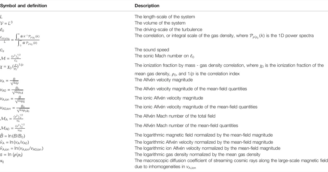
TABLE 1. Quantities and definitions used throughout this study.

2 Turbulence Simulations

2.1 Stochastically Driven Isothermal magnetohydrodynamic (MHD) Fluid Model

To understand the nature of Alfvén velocity fluctuations in MHD turbulence, we use a modified (see Methods section in Federrath et al., 2021) version of the flash code (Fryxell et al., 2000; Dubey et al., 2008), utilizing a second-order conservative MUSCL-Hancock 5-wave approximate Riemann scheme (Bouchut et al., 2010; Waagan et al., 2011; Federrath et al., 2021) to solve the dimensionless 3D, ideal, isothermal, compressible MHD equations with a stochastic acceleration field acting to drive the turbulence with finite temporal correlation.

Where v is the fluid velocity, ρ is the gas density, $\mathbf{B}=B_0\widehat{\mathbf{z}}+\delta \mathbf{B}(t)$ is the magnetic field, with large-scale field $B_0\widehat{\mathbf{z}}$ and turbulent field δB, c_s is the sound speed, and f the stochastic turbulent acceleration source term that drives the turbulence. We solve the equations on a periodic domain of dimension $L^3\equiv \mathcal{V}$, discretised with between 16³–288³ cells for the purpose of ensuring the convergence of numerical quantities used in this study. All of the quantities reported in the main text are for 53 unique simulations at 288³, which we list in Table 2. We show sample slices through some of the simulations in Figure 1. At a resolution of 288³ grid cells, the simulations have numerically converged 2^nd-moment statistics (see Supplementary Section 6.2 for a numerical convergence test of the main statistics in this study), because the variance of the 3D turbulent fields is dominated by the lowest k-modes in the turbulence (see also Kitsionas et al., 2009).

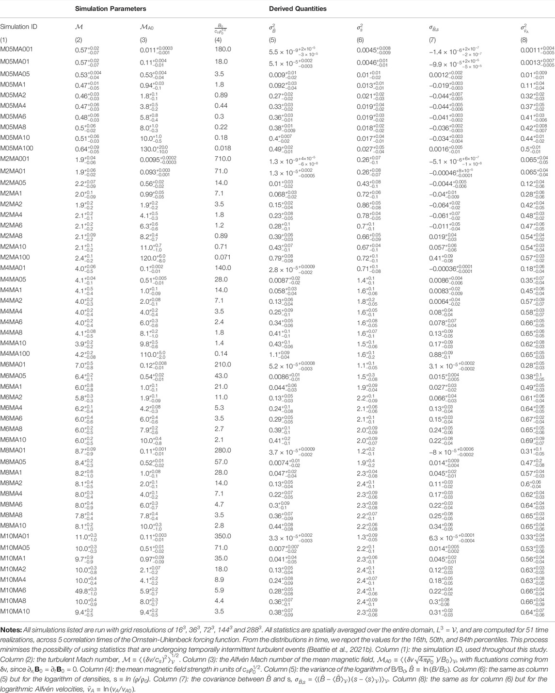
TABLE 2. Main simulation parameters and derived quantities used throughout this study.

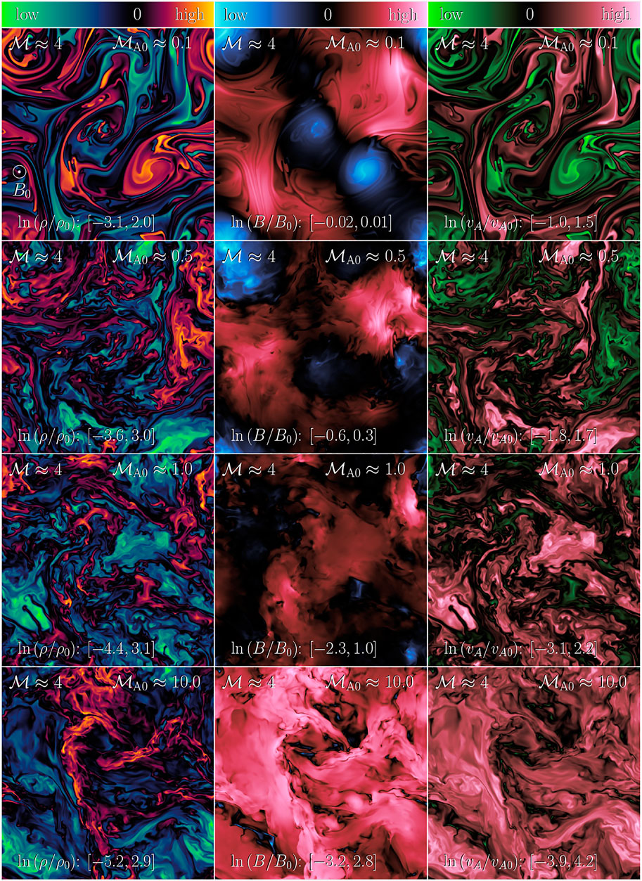
FIGURE 1. Two-dimensional slices through the logarithmic gas density, ln (ρ/ρ₀) (first column), logarithmic magnetic field, ln (B/B₀) (center column) and logarithmic Alfvén velocity magnitude, ln (v_A/v_A0) (third column) for $\mathcal{M}=4$ simulations. For each panel shown, simulation Mach and Alfvén Mach numbers are listed at the top, and the range covered by the color bar is indicated in brackets at the bottom. The slices are taken perpendicular to the large-scale field, B₀, which is pointing out of slice plane, as indicated in the top-left panel. The first three rows highlight the spatial correlation between the three field variables for the sub-to-trans-Alfvénic regime $({\mathcal{M}}_{\text{A0}}\lesssim 1)$, and the last row for the super-Alfvénic regime $({\mathcal{M}}_{\text{A0}}>1)$. For the sub-to-trans-Alfvénic, the spatial structure in ln (v_A/v_A0) ∼ ln (ρ/ρ₀), but as ${\mathcal{M}}_{\text{A0}}$ grows ln (v_A/v_A0) begins to more closely match ln (B/B₀).

2.2 Turbulent Driving and Sonic Mach Numbers

The forcing term f follows an Ornstein-Uhlenbeck process that satisfies the stochastic differential equation,

where $\widehat{\mathbf{f}}(\mathbf{k},t)$ is the Fourier transform of f, with correlation time, such that $\widehat{\mathbf{f}}(\mathbf{k},t)\sim f_0(\mathbf{k})\exp \left\{-t/\tau \right\}$ and $\tau ={\ell }_0/{⟨v^2⟩}_{\mathcal{V}}^{1/2}=L/(2c_s\mathcal{M})$ where ℓ₀ = L/2 is the energy injection scale. Every τ the driving field loses 1/e of its previous structure. By controlling τ we are able to set $0.5\lesssim \mathcal{M}\lesssim 10$, encapsulating the $\mathcal{M}$ values of supersonic molecular gas clouds in the interstellar medium (e.g., Schneider et al., 2013; Federrath et al., 2016; Orkisz et al., 2017; Beattie et al., 2019) as well as in the sub-sonic, diffuse medium (e.g., Kritsuk et al., 2017; Marchal and Miville-Deschênes, 2021). d W(t) is a Wiener process which draws delta-correlated random Gaussian increments from $\mathcal{N}(0,\mathrm{d}t)$, a mean-zero Gaussian distribution with variance d t, which is then projected onto f isotropically in k-space with amplitude f₀(k). A filter is chosen such that the driving spectrum is concentrated at |kL/2π| = 2 and falls off to zero with a parabolic spectrum between 1 ≤ |kL/2π| ≤ 3. The projection is performed using the projection tensor

where δ_ij is the Kronecker delta tensor. We control the contribution from each of the driving modes, indicated with the annotations for the two terms in the projection tensor, through the η parameter. For η = 1 we obtain purely solenoidal driving (∇ ⋅ f = 0), and η = 0 produces purely compressive driving (∇ × f = 0) (see Federrath et al., 2008; Federrath et al., 2009; 2010; Federrath et al., 2022, for a detailed discussion of the driving). We choose to inject an equal amount of energy in both compressive and solenoidal modes, a “natural mix”, by setting η = 0.5 (see Federrath et al., 2008; Federrath et al., 2009; 2010, for turbulence driving details). A natural mixture of modes is most appropriate for simulating ISM turbulence because driving mechanisms⁵ are diverse, for example, supernova shocks (compressive), internal instabilities in the gas (solenoidal), gravity (compressive), galactic shear (solenoidal), ambient pressure from the galactic environment (compressive) or stellar feedback (compressive or solenoidal) (Brunt et al., 2009; Elmegreen, 2009; Federrath, 2015; Krumholz and Burkhart, 2016; Federrath et al., 2017; Grisdale et al., 2017; Jin et al., 2017; Körtgen et al., 2017; Colling et al., 2018; Schruba et al., 2019; Lu et al., 2020)⁶.

2.3 Initial Conditions, Magnetic Field and Critical Balance

${\mathcal{M}}_{\text{A0}}$ is set by fixing B₀, which we do when we set up the turbulent boxes, and using the definition of the mean-field Alfvén velocity, $v_{\text{A0}}=B_0/{(4\pi {\rho }_0)}^{1/2}$ with respect to the mean field B₀, and $\mathcal{M}$. Thus, ${\mathcal{M}}_{\text{A0}}=c_s\mathcal{M}/v_{\text{A0}}=2c_s\sqrt{\pi {\rho }_0}\mathcal{M}/B_0$. We vary this value for each of the simulations between $10^{-2}\lesssim {\mathcal{M}}_{\text{A0}}\lesssim 10^2$. ${\mathcal{M}}_{\text{A0}}$ is almost a constant in time, since B₀ is constant, but because $\mathcal{M}$ fluctuates, so does ${\mathcal{M}}_{\text{A0}}$. Regardless, we find that the desired value of ${\mathcal{M}}_{\text{A0}}$ and the measured value closely match, as shown in the 2^nd column of Table 2. The initial velocity field is set to |v (x, y, z, t = 0)| = 0, with units c_s = 1, the density field ρ(x, y, z, t = 0)/ρ₀ = 1, with units ρ₀ = 1 and $|\delta \mathbf{B}(x,y,z,t=0)|/(c_s{\rho }_0^{1/2})=0$, with units $c_s{\rho }_0^{1/2}=1$. The turbulent magnetic field evolves self-consistently with the MHD fluid equations and satisfies ${⟨\delta \mathbf{B}(t)⟩}_{\mathcal{V}}=0$, or more generally, ${⟨\mathbf{B}(t)⟩}_{\mathcal{V}}=B_0$. This means ∂_xB₀ = ∂_yB₀ = ∂_zB₀ = ∂_tB₀ = 0, by construction. To ensure that the magnetic field is divergence-free, we use the parabolic ∇ ⋅B diffusion method described by Marder (1987).

Classifying the turbulence as weak or strong is beneficial for understanding the underlying turbulence phenomenology and statistics (Sridhar and Goldreich, 1994; Goldreich and Sridhar, 1995; Perez and Boldyrev, 2008; Boldyrev and Perez, 2009; Oughton and Matthaeus, 2020; Schekochihin, 2020). The critical balance parameter on the driving scale is ${\zeta }_{\text{crit}}\sim t_{\text{alfven}}/\tau \sim ({\ell }_{\Vert }/v_{A0}){({\ell }_0/c_s\mathcal{M})}^{-1}$ (Goldreich and Sridhar, 1995; Oughton and Matthaeus, 2020), where ℓ_‖ = ℓ₀ for isotropic driving, and hence ${\zeta }_{\text{crit}}\sim c_s\mathcal{M}/v_{\text{A0}}={\mathcal{M}}_{\text{A0}}$. Based on these simple arguments, on the outer scale of the turbulence, the ${\mathcal{M}}_{\text{A0}}<1$ ensemble of simulations may be considered weak (wave turbulence), and the ${\mathcal{M}}_{\text{A0}}\ge 1$ may be considered strong. However, we urge caution in interpreting our simulations under the strong and weak phenomenologies in relation to the parameters chosen for our simulations, because even though the ${\mathcal{M}}_{\text{A0}}<1$ simulations may seem weak, we are injecting compressible modes isotropically in k-space into the turbulence to mimic astrophysical sources of driving. This creates strong shocks and rarefactions that form along field lines in the ${\mathcal{M}}_{\text{A0}}<1$ turbulence, which are discussed more in Section 3 and visualized in Supplementary Figure S1. The presence of shocks (which are non-local in k-space) that evolve on very short timescales (e.g, shorter than the local sound crossing time, Robertson and Goldreich, 2018; Mocz and Burkhart, 2018) means that in many regions of the plasma non-linear effects cannot be neglected. This may prevent the turbulence from ever becoming truly weak.

2.4 Stationarity and Collecting Statistics

We run the simulations for 10τ, and report statistics from quantiles for the 50th, 16th and 84th percentiles of the time distributions over the last 5τ. This 1 ensures that the sub-Alfvénic, large-scale field simulations are statistically stationary, i.e., ${⟨\mathbf{X}(t)⟩}_{\mathcal{V}}={⟨\mathbf{X}(t+\mathrm{\Delta }t)⟩}_{\mathcal{V}}$, for an arbitrary field variable X, and increment in time Δt, which takes roughly 5τ for those experiments (Beattie et al., 2021b)⁷ and 2 makes all of our results robust to temporally intermittent events, which are ubiquitous in turbulence experiments. Unless explicitly written, we will average every statistic in this study, including 1D and 2D PDFs in Sections 3.1–3.3, to make sure our results are as robust as possible. Throughout the study we use a naming convention for our simulations whereby the value following the M gives the target $\mathcal{M}$ (with omitted decimal points) and the value following MA gives the target ${\mathcal{M}}_{\text{A0}}$ – thus run M10MA01 is one where we set the large-scale magnetic field Alfvén Mach number to ${\mathcal{M}}_{\text{A0}}=0.1$ and tune the correlation time of the stochastic forcing to produce a sonic Mach number of $\mathcal{M}=10$. Now we turn to the results of this study.

3 Ionic Alfvén Velocity Fluctuations

Consider the dimensionless magnitude of the ionic Alfvén velocities in a magnetized, compressible plasma,

The correlation between the gas density and the ionization fraction is,

where χ₀ is the mass ionization fraction at density ρ₀. When p → ∞ ⇒ χ = χ₀, the equilibrium time between ionizing the plasma t_ion and a typical density fluctuation $t_{\rho /{\rho }_0}$ is comparable $t_{\text{ion}}\sim t_{\rho /{\rho }_0}$ (warm atomic gas), and for p = 2, $t_{\text{ion}}\ll t_{\rho /{\rho }_0}$ (cold molecular or atomic gas), following Eq. 2; ideal MHD is χ₀ = 1, p → ∞. For a general p > 0,

where

We make this change of variables to bring out the symmetry in the log transform of v_A,ion,

where s = ln (ρ/ρ₀), ${\tilde{v}}_{\text{A,ion}}=\ln (v_{A,\mathrm{i}\mathrm{o}\mathrm{n}}/v_{A0,\mathrm{i}\mathrm{o}\mathrm{n}})$ and $v_{A0,\mathrm{i}\mathrm{o}\mathrm{n}}=B_0/(c_s\sqrt{4\pi {\rho }_0{\chi }_0})$. Now ${\tilde{v}}_{\text{A,ion}}$ is simply the addition of two random variables, $\tilde{B}$ and − [(p − 1)/(2p)]s. This means the ${\tilde{v}}_{\text{A,ion}}$ variance is

where ${\sigma }_{\tilde{B},s}$ is the spatial covariance between $\tilde{B}$ and s,

Thus, if we want to model the PDF and variance of ${\tilde{v}}_{\text{A,ion}}$, and in turn, v_A,ion, we must understand ${\sigma }_{\tilde{B}}^2$, ${\sigma }_s^2$, and the covariance between them. Hence, before we focus our attention on Alfvén speed fluctuations themselves, we first consider the three necessary ingredients: density and magnetic field fluctuations and the correlations between them. We start with density fluctuations.

3.1 Density Fluctuations

In Figure 2 we show the s-PDFs from the ${\mathcal{M}}_{\text{A0}}=0.1$ (left), ${\mathcal{M}}_{\text{A0}}=1.0$ (middle) and ${\mathcal{M}}_{\text{A0}}=10.0$ (right) simulations, colored by $\mathcal{M}$. From $\mathcal{M}=0.5-4$, the s-PDF monotonically increases with $\mathcal{M}$, showing how the amplitude and dispersion in density fluctuations becomes greater as the compressibility in the magnetized plasma increases, regardless of ${\mathcal{M}}_{\text{A0}}$, as shown previously in Molina et al. (2012) and Beattie et al. (2021a,b). At $\mathcal{M}\gtrsim 4$ the spread of the s-PDFs begins to slow, which is not found in hydrodynamical compressible turbulence (see Figure 1 in Price et al., 2011) but has been explained in Molina et al. (2012) and Beattie et al. (2021b) as due to correlations between the magnetic field and density field growing, and “cushioning” the plasma, preventing it from creating strong over-and-under-densities. These correlations become important for v_A, which we will discuss and explore in more detail in Section 3. Overall, as $\mathcal{M}$ increases, the PDFs become more negatively skewed as the plasma becomes rich in volume-filling rarefactions. This is because the characteristic thickness of an over-dense region scales with $\sim {\ell }_0/{\mathcal{M}}^2$ (Padoan et al., 1997; Molina et al., 2012; Mocz and Burkhart, 2018; Robertson and Goldreich, 2018), and hence, as $\mathcal{M}$ increases the shocked gas becomes less volume-filling (skewing the PDFs), but contains most of the mass in the plasma (Robertson and Goldreich, 2018; Beattie et al., 2021b).

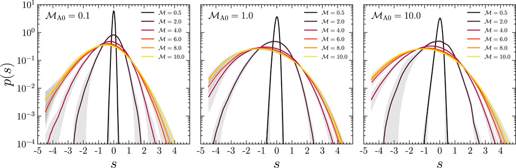
FIGURE 2. The logarithmic density PDFs for the sub-Alfvénic, ${\mathcal{M}}_{\text{A0}}=0.1$, simulations (left), trans-Alfvénic, ${\mathcal{M}}_{\text{A0}}=1.0$ simulations (middle), and super-Alfvénic, ${\mathcal{M}}_{\text{A0}}=10.0$, simulations (right), colored by $\mathcal{M}$. Between $0.5\le \mathcal{M}\le 4$ we find monotonic growth in the spread of the PDF, showing that as the flow becomes more compressible the density fluctuations increase in magnitude and dispersion. Beyond $\mathcal{M}\approx 4-6$, complex correlations between the density and magnetic field suppress the largest over- and under-densities (Molina et al., 2012; Beattie et al., 2021a,b), and the variance of the PDF stops growing.

In Figure 3 we show ${\sigma }_s^2$ for the entire ensemble of simulations utilised in this study, plotted as a function of $\mathcal{M}$. For reference, we also plot the relation from hydrodynamical supersonic turbulence theory (dashed, red),

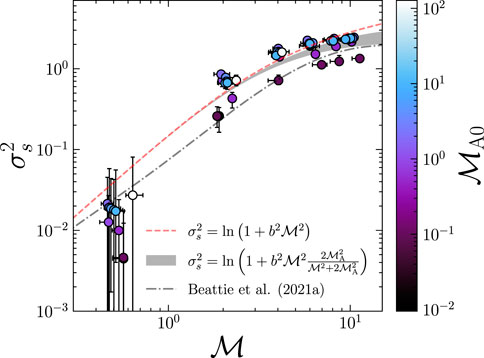
FIGURE 3. The logarithmic density variance, ${\sigma }_s^2$ as a function of $\mathcal{M}$, colored by ${\mathcal{M}}_{\text{A0}}$. We show the hydrodynamical model of the variance, ${\sigma }_s^2=\ln (1+b^2{\mathcal{M}}^2)$ (Federrath et al., 2008; Federrath et al., 2010), shown with the red, dashed line, the Molina et al. (2012) model, ${\sigma }_s^2=\ln (1+b^2{\mathcal{M}}^2[2{\mathcal{M}}_{\text{A}}/({\mathcal{M}}^2+2{\mathcal{M}}_{\text{A}}^2)])$, which corrects for magnetic pressure, evaluated between ${\mathcal{M}}_{\text{A0}}=6-10$ with the gray band, and the Beattie et al. (2021a) model, which corrects for the anisotropic nature of sub-Alfvénic density fluctuations, evaluated at ${\mathcal{M}}_{\text{A}}=0.1$ with the gray dashed-dotted line. The variance models describe the data well for $\mathcal{M}\gtrsim 2$ but become worse as $\mathcal{M}$ decreases, where the compressible modes are unable to create significant density fluctuations.

(Federrath et al., 2008; Federrath et al., 2010), super-Alfvénic MHD turbulence theory (gray band),

assuming ρ ∝ B^1/2 (Molina et al., 2012) evaluated between ${\mathcal{M}}_{\text{A0}}=2-10$, and sub-Alfvénic MHD turbulence theory (dot-dashed, gray).

Where, ${\mathcal{V}}_0$ is the volume-filling fraction of shocked gas along B₀ in the trans-sonic limit and ${\mathcal{M}}_{\text{c}}$ is the critical $\mathcal{M}$ where the volume-filling fraction of the gas along B₀ becomes negligible (Beattie et al., 2021a). As with Figure 2, regardless of ${\mathcal{M}}_{\text{A0}}$, ${\sigma }_s^2$ shows qualitatively similar behavior–becoming monotonically more weakly dependent upon $\mathcal{M}$ as $\mathcal{M}$ increases, following the logarithmic trend captured by the density variance models. However, as $\mathcal{M}$ increases, the sub-Alfvénic experiments settle to values roughly a factor of 2 lower in ${\sigma }_s^2$ than both the super-Alfvénic experiments and the prediction from the hydrodynamical variance model (shown with the red-dashed lines). For these sub-Alfvénic plasmas, Beattie et al. (2021a) attributed the stronger flattening of the variance to fluctuations along the B₀⁸ (uncorrelated, ρ ∝ B⁰) becoming extremely low volume-filling, and the fluctuations across the field lines (ρ ∝ B) becoming the dominant source of volume-weighted variance. Since ρ ∝ B fluctuations have to perturb the magnetic field, and because B₀ is very strong in the sub-Alfvénic regime, these are weak fluctuations that do not grow the variance as fast as the ρ ∝ B⁰ fluctuations.

The key point is that, regardless of $\mathcal{M}$ and ${\mathcal{M}}_{\text{A0}}$, the lognormal model for the density PDF is a reasonable (and practical) approximation to make. Equipped with this knowledge, we now move on to the second ingredient we need to understand the nature of Alfvén wave fluctuations in compressible MHD turbulence—the magnetic field fluctuations.

3.2 Magnetic Field Fluctuations

In a similar treatment as the last section, we plot a representative sample of the logarithmic magnetic magnitude PDFs in Figure 4 on the same scale as the PDFs shown in Figure 2. Unlike the s-PDFs, the $\tilde{B}$-PDFs show a very strong dependence upon the strength of the large-scale magnetic field (or likewise, ${\mathcal{M}}_{\text{A0}}$) and only a weak dependence upon $\mathcal{M}$. In the sub-Alfvénic regime (left panel) the magnetic field resembles a delta function centered on the value of large-scale field, ln (B/B₀) = 0. As ${\mathcal{M}}_{\text{A0}}$ increases, and the strength of the large-scale field decreases the turbulent component of the magnetic field is able to grow, and we can observe some structure in the $\tilde{B}$-PDFs. At ${\mathcal{M}}_{\text{A0}}=1$, B₀ is still dominant ($\delta B^2/B_0^2=1$ at ${\mathcal{M}}_{\text{A0}}=2$, Beattie et al., 2020, 2022), however small asymmetries between volumes with B > B₀ and B < B₀ develop and negatively skew the PDF. These features become extremely pronounced at ${\mathcal{M}}_{\text{A0}}=10.0$ (similar non-Gaussian features are very pronounced for ${\mathcal{M}}_{\text{A0}}=\infty$; Seta and Federrath, 2021a), where $\delta B^2\gg B_0^2$, and hence, when the nonlinear terms in the fluid equations are the strongest (Oughton et al., 1994).

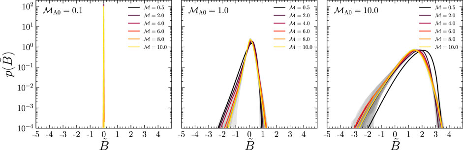
FIGURE 4. The same as Figure 2, but for the logarithmic magnetic field magnitudes. For ${\mathcal{M}}_{\text{A0}}<1$, the distribution is dominated by B₀, with negligible fluctuations. As ${\mathcal{M}}_{\text{A0}}$ increases, and B₀ decreases, the turbulent component of the field grows and the distribution spreads out and becomes negatively skewed. The tails and median of the distribution are weakly dependent upon $\mathcal{M}$. The negative skewness grows with ${\mathcal{M}}_{\text{A0}}$ (weakening B₀), indicating that more of the simulation volume is filling with highly-tangled magnetic fields, which produce magnetic field magnitudes larger than B₀.

Not only are the higher-order moments of the PDFs growing with ${\mathcal{M}}_{\text{A0}}$, but the volume-weighted $\tilde{B}$-PDFs shift to higher values of $\tilde{B}$, with most values B > B₀, as ${\mathcal{M}}_{\text{A0}}$ increases. This means that when the large-scale field is weak, the turbulence is able to feed the fluctuating magnetic field with energy, growing most of the field beyond B₀. As shown in Figure 2 of Beattie and Federrath (2020), the topology of the magnetic field becomes extremely tangled and complex. It is well known that tangling, or knotting the field, by increasing the number of crossings between flux tubes grows the magnetic energy linearly with number of crossings⁹ (Freedman and He, 1991; Seligman et al., 2022). The net result of this is that the magnetic field becomes tangled, paths along field lines become volume-filling, and B > B₀ in most of the fluid volume. The middle column of Figure 1 shows exactly this: as ${\mathcal{M}}_{\text{A0}}$ increases from 0.1 to 10.0, the amount of pink (B/B₀ > 1) compared to blue (B/B₀ < 1) increases and becomes volume-filling. In contrast to the s variance, there is much less theory on the magnetic field variance. However, recent works have had some success in understanding the B/B₀ (linear magnetic field) variance. Next we summarise those results and compare them to our simulation data.

We plot the variance of both the linear, large-scale field normalized magnetic field B/B₀ (left panel) and logarithmic magnetic field (right panel) of Figure 5. Both plots show a systematic power law increase with ${\mathcal{M}}_{\text{A0}}$, with a break scale between ${\mathcal{M}}_{\text{A0}}\approx 1-2$. This marks the energy equipartition transition between the turbulent magnetic field energy and large-scale magnetic field energy. For the linear field, we utilize the models developed in Beattie et al. (2022). They find that by taking the 2^nd moments of the energy balance between the magnetic and kinetic energy,

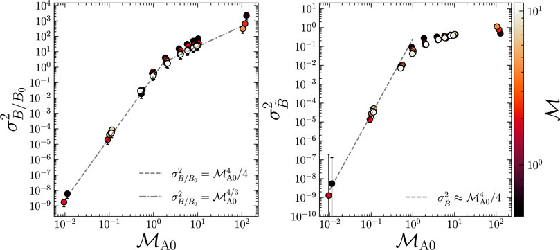
FIGURE 5. The variance of B/B₀ (left) and ln (B/B₀) (right) as a function of ${\mathcal{M}}_{\text{A0}}$, colored by $\mathcal{M}$. In the left panel, we plot the B/B₀ variance models (gray-dashed lines) derived through energy balance arguments in Beattie et al. (2022), which capture both the sub-Alfvénic and super-Alfvénic regime. For ${\sigma }_{\tilde{B}}^2$, in the right panel, we use the delta method to derive the variance in the sub-Alfvénic regime, which, to linear order, is equal to ${\sigma }_{B/B_0}^2$.

relations between the rms magnetic field, including the effects of the large-scale field via the δB ⋅B₀ term in the above equation, can be derived without any use of fitting parameters. For the variance of B/B₀, this results in,

which show excellent agreement with the simulation data, across all ${\mathcal{M}}_{\text{A0}}$ and $\mathcal{M}$. Note also that ${\mathcal{M}}_{\text{A}}\approx {\mathcal{M}}_{\text{A0}}$ when ${\mathcal{M}}_{\text{A0}}\le 2$ (Beattie et al., 2022), and ${\mathcal{M}}_{\text{A}}$ is an observable quantity using Davis (1951), Chandrasekhar and Fermi (1953) and Skalidis and Tassis (2020) starlight polarization methods, hence, in principle, ${\sigma }_{B/B_0}^2$ is a derivable quantity from observations. We discuss this more in Section 4. However, Eq. 21 critically depends upon the $\tilde{B}$ variance, and not the ${\sigma }_{B/B_0}^2$. Using the delta method (see, e.g., Hoef, 2012, for a summary of the method), one can approximate the moments of functions of random variables utilizing the Taylor expansion of the function. To linear order, the variance is, $\text{Var}\left\{f(X)\right\}={\left[{\partial }_{X}f(⟨X⟩)\right]}^2\text{Var}\left\{X\right\}$, where $\text{Var}\left\{X\right\}$ is the variance operator applied to random variable X. In our case, X = B/B₀ and hence $⟨B/B_0⟩=1$, and ${\partial }_{B/B_0}\ln (⟨B/B_0⟩)=1$. This means, to linear order, ${\sigma }_{\tilde{B}}^2={\sigma }_{B/B_0}^2$. But, the delta method only works well for $\text{Var}\left\{B/B_0\right\}/⟨B/B_0⟩<1$, hence we are only able to apply this approximation in the sub-Alfvénic regime, where this condition is met. We plot this function in the right panel of Figure 5, which shows reasonable agreement with the data up until ${\sigma }_{\tilde{B}}^2\approx 0.1$, which corresponds to ${\mathcal{M}}_{\text{A0}}=1$.

3.3 Covariance Between the Magnetic and Density Fluctuations

In the last two sections we developed an understanding of the global fluctuations (the variance) of the logarithmic density and magnetic field fluctuations. It may already be apparent that in the sub-Alfvénic regime the magnetic field fluctuations are completely negligible, and for ${\tilde{v}}_{\text{A,ion}}$, the density fluctuations are going to be dominant. To make this more quantitative, we plot the ratio of the s and $\tilde{B}$ variances in the left panel of Figure 6. As expected ${\sigma }_s^2\gg {\sigma }_{\tilde{B}}^2$ in the sub-Alfvénic regime, by up to nine orders of magnitude at ${\mathcal{M}}_{\text{A0}}=0.01$ down to two orders of magnitude at ${\mathcal{M}}_{\text{A0}}=1.0$. Between $\mathcal{M}=2$ and $\mathcal{M}=10$ there is roughly an order of magnitude difference, with the s fluctuations playing a larger role with increasing $\mathcal{M}$. This highlights the importance of compressibility in the sub-Alfvénic regime, in particular, where the $\tilde{B}$ fluctuations have orders of magnitude less power than the s fluctuations.

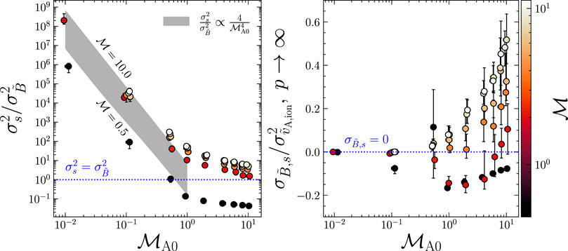
FIGURE 6. Left: The logarithmic density and magnetic field variance ratio as a function of ${\mathcal{M}}_{\text{A0}}$, colored by $\mathcal{M}$. In ${\mathcal{M}}_{\text{A0}}<1$ regime, the s fluctuations are many orders of magnitude larger than the magnetic field fluctuations. As ${\mathcal{M}}_{\text{A0}}$ increases, the $\tilde{B}$ field fluctuations contribute more strongly to the ratio and the ratio flattens. If $\mathcal{M}<1$, then at high-${\mathcal{M}}_{\text{A0}}$ the $\tilde{B}$ fluctuations dominate, and vice versa for $\mathcal{M}>1$. Using the gray band, we plot the ratio between Eqs. 27, 29, which shows ${\sigma }_s^2/{\sigma }_{\tilde{B}}^2\propto {\mathcal{M}}_{\text{A0}}^{-4}$, for ${\mathcal{M}}_{\text{A0}}<1$. Right: The same as the left panel but for the covariance of the logarithmic magnetic field $\tilde{B}$ and density s weighted by the variance of the logarithmic ion Alfvén velocities (in the ideal limit p → ∞ and χ = χ₀ = 1). This statistic shows the magnitude of the correlations between the $\tilde{B}$ and s fields for the different strengths in large-scale magnetic field. At low-${\mathcal{M}}_{\text{A0}}$, the correlations are negligible, and hence $\tilde{B}$ and s are independent. However, for ${\mathcal{M}}_{\text{A0}}\approx 1$, the correlations contribute significantly to ${\sigma }_{{\tilde{v}}_{\text{A,ion}}}^2$.

Using the Beattie et al. (2021a) model for the s variance, Eq. 27, which we plotted in Figure 3, and the $\tilde{B}$ variance, Eq. 29, we use from Beattie et al. (2022), for the sub-Alfvénic regime, we get,

where the proportionality factor is Eq. 27, and for when the delta method for approximating ${\sigma }_{\tilde{B}}^2$ is valid. We plot this model evaluated at $\mathcal{M}=10$ and $\mathcal{M}=0.5$ with the gray band in Figure 6. The slope $\sim {\mathcal{M}}_{\text{A0}}^{-4}$ looks accurate, but the exact offset, which is a function of the ${\sigma }_s^2$ prescription, does not capture the subsonic regime properly, which makes sense because the ${\sigma }_s^2$ models are valid for the $\mathcal{M}>1$ regime, as discussed in Section 3.1. Regardless, the model describes the general trend, and is useful in that we now know ${\sigma }_s^2/{\sigma }_{\tilde{B}}^2\propto {\mathcal{M}}_{\text{A0}}^{-4}$, which highlights that in the sub-Alfvénic regime, it is the density fluctuations that are leading order in Eq. 21.

Of course comparing the first two terms in Eq. 21 is important to determine which is leading order, but if the covariance between the fields is large, then this will still complicate the modeling of ${\sigma }_{{\tilde{v}}_{\text{A,ion}}}^2$. Hence, in the right panel of Figure 6 we plot the ratio between the covariance of $\tilde{B}$ and s and ${\sigma }_{{\tilde{v}}_{\text{A,ion}}}^2$. This gives us an idea of the magnitude of the covariance contribution to ${\sigma }_{{\tilde{v}}_{\text{A,ion}}}^2$. For ${\mathcal{M}}_{\text{A0}}<1$, we find that the covariance term is negligible, ${\sigma }_{\tilde{B},s}\approx 0$. As discussed more qualitatively in Molina et al. (2012) and Beattie et al. (2021b) (and previously in Section 3.1), as ${\mathcal{M}}_{\text{A0}}$ gets larger, the covariance (correlations between the magnetic and density field) begins to become sensitive to $\mathcal{M}$. For the supersonic simulations, the covariance is positive, and makes the largest contributions for the highest $\mathcal{M}$, ${\sigma }_{\tilde{B},s}\approx (0.5-0.6){\sigma }_{{\tilde{v}}_{\text{A}}}^2$. This is qualitatively similar to previous results involving measuring the correlations between density and magnetic properties of supersonic turbulence (e.g., Burkhart et al., 2009; Yoon et al., 2016). Most likely this comes about from flux-freezing and compressive motions that lead to the over-dense, highly-magnetized regions that we show in the last row of Figure 1. Because of the extra magnetic pressure, and the strong correlations, this also means that it is hard to create large compressions, which is why the variance of the s-PDF grows more slowly than in hydrodynamical turbulence, as discussed in Section 3.1.

In contrast, the sub (to-trans)sonic, super-Alfvénic experiments give rise to a negative covariance. This could mean either the magnetic field is strong in under-densities, or the field is weak in over-densities, or both. If one carefully analyses the s-PDF and the $\tilde{B}$-PDF, then one can see that it is under-densities where the magnetic field becomes strong, and if it were over-densities giving rise to a weak magnetic field the s-PDF would need to be skewed in the opposite direction given the negative skewness in the $\mathcal{M}=0.5\tilde{B}$-PDF. Previous experiments have concluded that this is due to a thermal, $(1/{\mathcal{M}}^2)\nabla c_s\rho$, and magnetic pressure, $(1/{\mathcal{M}}_{\text{A}}^2)\nabla B^2$, balance, ${\mathcal{M}}_{\text{A}}\approx \mathcal{M}$, that allows the fluid to equilibriate on shorter timescales than the correlation times in subsonic turbulence (Yoon et al., 2016). This amounts to regions of strong magnetization evacuating the gas density until the thermal pressure back-reacts and an equilibrium is reached. Of course, when $\mathcal{M}\gg 1$, the thermal pressure becomes less important and the short correlation timescales in the turbulence do not give the plasma a large enough correlated time interval to undergo such a process. Based on Figure 6, $\mathcal{M}\approx 2-4$ defines the critical $\mathcal{M}$ for when the equilibration time is shorter than the correlation time of the turbulence.

To understand these correlations (or lack thereof) further, we plot the time-averaged joint distributions of − [(p − 1)/2p]s and $\tilde{B}$ in Figure 7 in the limit where p → ∞ and χ = χ₀ = 1, which gives,

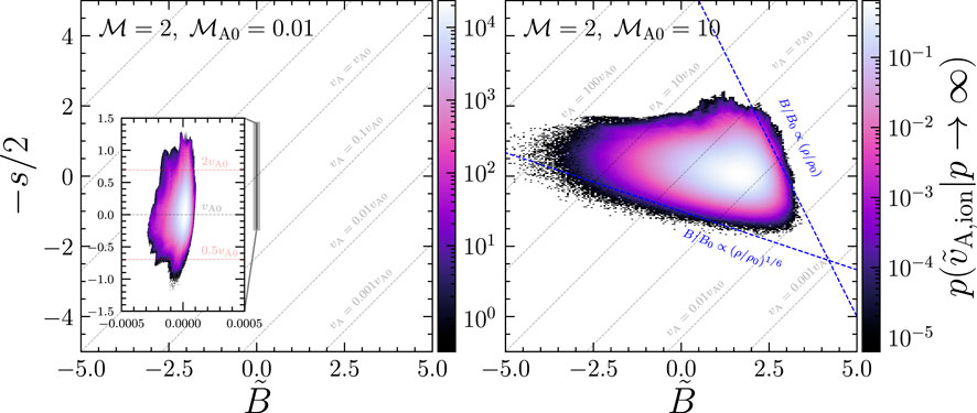
FIGURE 7. The joint $\tilde{B}\equiv \ln (B/B_0)$ and − s/2 ≡ − 1/2 ln (ρ/ρ₀) PDFs, which we demonstrate is the ${\tilde{v}}_{\text{A,ion}}$-PDF in the χ = χ₀ = 1 and p → ∞ limit, Eq. 31. We show gray lines of constant v_A in units of v_A0. Each line represents a change in v_A by an order of magnitude in v_A0. Left: the joint PDF for the M2MA001 simulation, showing that in the sub-Alfvénic regime the variation in ${\tilde{v}}_{\text{A,ion}}$ is determined solely by the density fluctuations, and that the $\tilde{B}$ and s fluctuations can be treated as independent. The mechanism for creating density fluctuations independent of the magnetic field are from channel flows along the field lines that compress the fluid into perpendicular filaments along B₀ (Beattie and Federrath, 2020; Beattie et al., 2021b). Right: the same as the left panel but for the super-Alfvénic M2MA10 simulation, revealing significant variation in both the $\tilde{B}$ and s fluctuations, with some rough correlations enveloping the PDF that we add to guide the eye.

to compare directly with our simulation data. The benefit of making this joint PDF, as opposed to B versus ρ, or B² versus ρ, is that lines in this space have constant Alfvén velocity magnitudes, as shown in Eq. 21, and the probability density is then exactly the probability density of ${\tilde{v}}_{\text{A,ion}}$, which is the quantity of interest in our study. Because − s/2 is negative, positive correlations in the plot go down the − s/2 axis. We plot the joint PDF for a highly sub-Alfvénic simulation, M2MA001 on the left, and a super-Alfvénic simulation, M2MA10, on the right, with constant Alfvén velocities in units of the mean-field Alfvén velocities shown with gray contours in both plots, and blue lines for correlations between B/B₀ and ρ/ρ₀ that define the envelopes of the PDF for the super-Alfvénic data.

To be able to visualize the structure in the sub-Alfvénic data, we require a zoom-in to see the variation in $\tilde{B}$, which we show with the inset panel. The PDF varies over $\mathcal{O}(10^{-4})$ in $\tilde{B}$ compared to $\mathcal{O}(10^{-1})$ for s, consistent with all of the other results presented in this study. As we found with the covariance, there is no systematic change orientation in the $-s/2-\tilde{B}$ plane for the sub-Alfvénic data, which means that s and $\tilde{B}$ are independent. The physical reason why this is the case in the sub-Alfvénic regime is simple. Because the large-scale field is so strong, and is unable to be bent by the turbulence (sub-Alfvénic large-scale turbulence naturally implies $B_0^2\gg \delta v^2$), through flux-freezing, density fluctuations can only form from compressible velocity channels up and down magnetic field lines¹⁰, where both B and ρ are uncorrelated from one another. These channels are very important for turbulence in the ISM that may be sub-Alfvénic, because through the converging channel flows the plasma is able to compress the gas, essentially with hydrodynamical shock-jump conditions, $\rho /{\rho }_0\sim {\mathcal{M}}^2$ (Mocz and Burkhart, 2018; Beattie et al., 2021b), allowing for very dense filaments that form perpendicular to B₀, which undoubtedly become the sites of star formation in sub-Alfvénic star-forming molecular clouds (Padoan and Nordlund, 1999; Chen and Ostriker, 2014; Abe et al., 2020; Bonne et al., 2020; Chen et al., 2020). Clearly, based on the joint PDF, this is the sole mechanism for forming strong over-densities in the highly sub-Alfvénic regime, and hence, the sole mechanism for creating dispersion in the Alfvén velocities.

The super-Alfvénic data shows a wide spread in $\tilde{B}$ and s values, with a B/B₀ ∝ ρ/ρ₀ correlation at large B amplitudes, corresponding to compressions perpendicular to magnetic field lines (e.g., Tritsis et al., 2015), and a weak $B/B_0\propto {(\rho /{\rho }_0)}^{1/6}$ correlation at low-s, possibly due to the tangled field. Clearly the super-Alfvénic turbulence is full of a mixture of correlations as volume-filling tangled fields interact with networks of shocked gas, rarefactions and voids. Finally, we note that all of the exact values for the correlations discussed in this section are sensitive to the driving routine and numerical methods, as highlighted by Yoon et al. (2016), but regardless of the numerical treatment, and the precise correlations, the most important point is that not only can we can treat s and $\tilde{B}$ independently in the sub-Alfvénic regime, but $p(\tilde{B})$ is fundamentally a delta distribution centered at zero. We will use both of these important results in the next section.

3.4 Constructing an Ionic Alfvén Velocity Fluctuation Model

Throughout the last two sections we have learned that the magnetic field fluctuations are extremely weak in sub-Alfvénic large-scale field turbulence and in fact negligible compared to the total power in the density fluctuations, as shown in the left panel of Figure 6. Furthermore, in this regime channel flows along B₀ are the only way to significantly shock the gas, which makes ${\sigma }_{\tilde{B}}^2$ and ${\sigma }_s^2$ independent of one another. These two observations mean Eq. 21 becomes simply

when it is completely determined by logarithmic density fluctuations.

We plot ${\sigma }_{{\tilde{v}}_{\text{A,ion}}}^2$ as a function of ${\sigma }_s^2$ in Figure 8 for both the χ = χ₀ = 1 case (p → ∞) and the χ ∝ ρ^−1/2, (p = 2) case, in the left and right panel, respectively. In the limit that all of the variation in ${\tilde{v}}_{\text{A,ion}}$ is explained by s-fluctuations, e.g., as appropriate for the sub-Alfvénic turbulent regime, Eq. 32 gives,

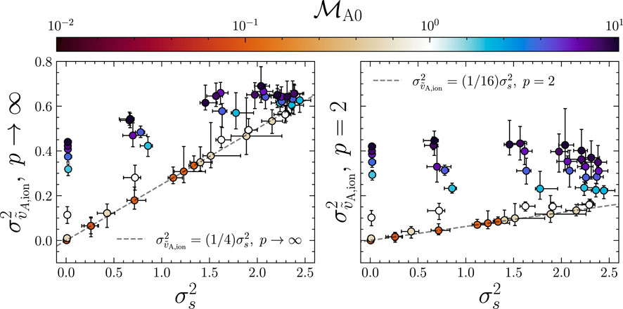
FIGURE 8. The logarithmic ion Alfvén velocity variance, ${\sigma }_{{\tilde{v}}_{\text{A,ion}}}^2$, as a function of logarithmic density variance, ${\sigma }_s^2$, colored by ${\mathcal{M}}_{\text{A0}}$. The color bar diverges around the sub-to-super Alfvénic transition, with ${\mathcal{M}}_{\text{A0}}<1$ colored red and ${\mathcal{M}}_{\text{A0}}>1$ colored blue., Left: the variance for the ionization state when the gas density is evolving on short enough timescales to not have enough time to reach ionization equilibrium (p → ∞). Right: the variance for when the gas is in ionization equilibrium (p = 2). The ${\sigma }_{{\tilde{v}}_{\text{A,ion}}}^2$ model (Eq. 33) is shown with a gray-dashed line, and indicates the case where the ion Alfvén velocity fluctuations are controlled completely by density fluctuations, and the density and magnetic field fluctuations are independent from one another. In the sub-to-trans-Alfvénic regime, where these conditions are met, this model is a good description of the data, across all of ${\sigma }_s^2$, and then for high-${\sigma }_s^2$ (high-$\mathcal{M}$) it gives a reasonable approximation, where the density fluctuations are strong. This highlights the importance of compressibility for understanding the ionic Alfvén velocity fluctuations.

and

which we plot with the dashed-gray lines in each panel of Figure 8. For both ionization states, as expected from our analysis in Section 3.2 and above, the sub-to-trans-Alfvénic simulations closely match the relation, showing that indeed the variances of the ion Alfvén speeds are being controlled by the density fluctuations¹¹. In the p → ∞ state, the super-Alfvénic experiments at higher ${\sigma }_s^2$ (higher $\mathcal{M}$) start approaching the relation, even though the correlations between s and $\tilde{B}$ are becoming significant (right panel of Figure 6). This is where the s-fluctuations are the strongest (the gas density is extremely inhomogenous) (e.g., Molina et al., 2012; Beattie et al., 2021a) and hence still significantly contribute to the dispersion of the Alfvén velocities.

Now that we have a variance model we move on to constructing the full ${\tilde{v}}_{\text{A,ion}}$-PDF, based on our previous results. Because s and $\tilde{B}$ are independent in the ${\mathcal{M}}_{\text{A0}}\lesssim 1$ regime, and $\tilde{B}$ is approximately a delta distribution centered at the zero, $\delta (\tilde{B})$, it follows that,

which, for a lognormal s-PDF (a reasonable approximation, as discussed in Section 3.1) ${\tilde{v}}_{\text{A,ion}}$ also becomes lognormal with − (p − 1)/(2p) propagated through the moments¹². It is

and under the lognormal formalism, is solely dependent upon the s variance, and ionization-density correlation χ ∝ ρ^−1/p. The strength of the 1/p correlation contracts (by a factor of [2p/(p − 1)]²) and shifts (by a factor of − [2p/(p − 1)]²/2, because $⟨{\tilde{v}}_{\text{A}}⟩=-{[2p/(p-1)]}^2/2{\sigma }_{{\tilde{v}}_{\text{A}}}^2$) the s-PDF, mapping the logarithmic densities into the Alfvén velocities. As the correlation increases, p → 0, the distribution approaches a delta distribution centered at zero, corresponding to no variation in the Alfvén velocities.

To compare with our data we take the limit in which p → ∞. This reduces Eqs. 36, 37 to

In Figure 9 we show fits of Eq. 38 for a representative sample of $\mathcal{M}$ and for the sub-to-trans-Alfvénic regime in the first three rows, and ${\mathcal{M}}_{\text{A0}}=10$ simulations in the final row, where we expect our model to be invalid. There is no fitting parameters in these PDF models, and they are solely determined by ${\sigma }_s^2$, which is measured independently in the data and fed into Eq. 38.

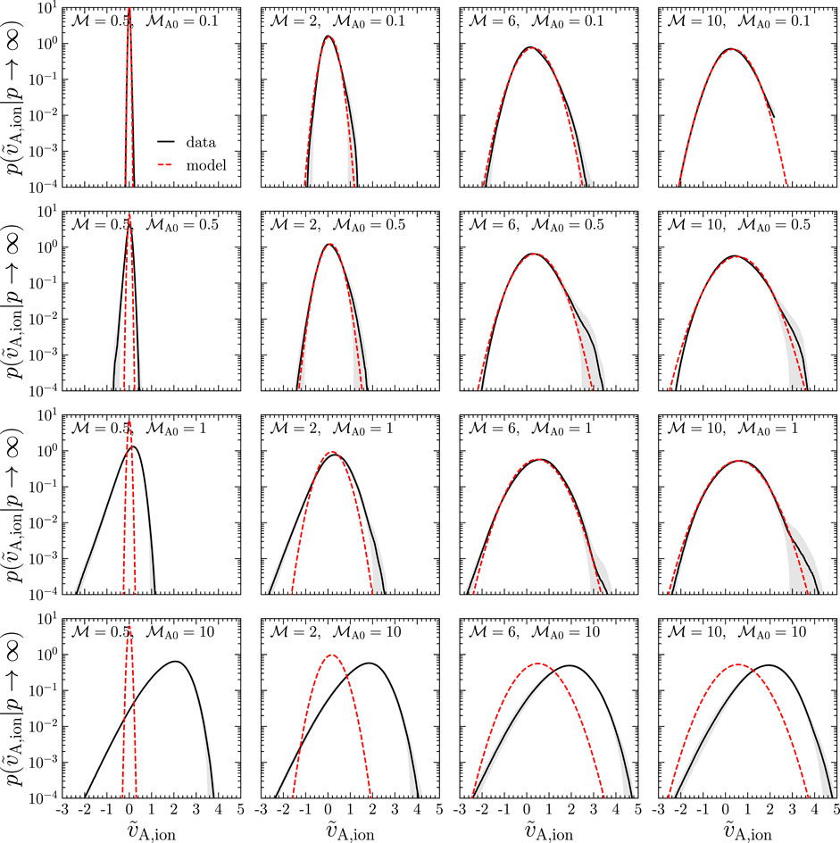
FIGURE 9. The volume-weighted logarithmic ion Alfvén velocity distribution for a selection of subsonic (left), supersonic (right) and sub-to-trans-Alfvénic (first three rows) simulations, shown in black, with 1σ fluctuations shown with the gray band. Our model, Eq. 38, is shown with the red dashed line, evaluated in the χ = χ₀ = 1 limit, corresponding to p → ∞ in Eq. 36. ${\mathcal{M}}_{\text{A0}}=10.0$ simulations are shown in the last row, where our model is predicted to not be valid. The deviations between our model and the data in these simulations showcases the affect of magnetic field fluctuations and correlations on the ${\tilde{v}}_{\text{A}}$-PDF.

In the sub-to-trans-Alfvénic regime, the most significant deviation is at small $\mathcal{M}$ (low-${\sigma }_s^2$ in Figure 8). This is because, as shown in both panels in Figure 6, the subsonic, trans-Alfvénic regime has stronger magnetic field fluctuations than density fluctuations. These broaden the ${\tilde{v}}_{\text{A}}$ more than predicted in Eq. 38 and imprint some of the negative skewness that we saw in Figure 4 on the ${\tilde{v}}_{\text{A}}$-PDF. Note also that for ${\mathcal{M}}_{\text{A0}}=1$, the $\mathcal{M}=0.5$ experiment has the strongest covariance, as shown in Figure 6, so there are also density and magnetic field correlations developing in the plasma that we do not account for in this PDF model. For the rest of the sub-to-trans-Alfvénic simulations, all of the models describe the data well, with slight underestimates (not significant at 1σ, shown with the gray bands) of the high-${\tilde{v}}_{\text{A}}$ tail. These might be due to B/B₀ > 1 regions in the plasma, where the Alfvén wave speeds can become very high. However, since the magnetic field fluctuations are very small, these are never very significant in this regime.

We also include ${\mathcal{M}}_{\text{A0}}=10$ simulations in the bottom row. Clearly, based on the results discussed in Section 3.1 and Section 3.2, Eq. 33 is not valid in this regime. However, we still are able to learn about the plasma when it is in this state. Similar to the sub-to-trans-Alfvénic experiments, the low-$\mathcal{M}$ simulations are the dominated by magnetic field fluctuations, and are described poorly by only the density fluctuations. However, variance of the ${\tilde{v}}_{\text{A,ion}}$-PDFs for $\mathcal{M}>2$ look reasonable (as also shown in the left panel of Figure 8) and it is just the mean that is not properly captured by the model. From Figure 4 and discussed in Section 3.2, we know that the mean in the $\tilde{B}$-PDFs shifts with ${\mathcal{M}}_{\text{A0}}$ and not $\mathcal{M}$. This means it is likely that the shift in the ${\tilde{v}}_{\text{A,ion}}$-PDFs is from the tangled magnetic field growing the Alfvén velocities everywhere in the plasma, even though the variance is still being controlled largely by the density inhomogeneities.

We have now created a model for the PDF and variance of the logarithm of the Alfvén velocities that works over a broad range of $\mathcal{M}$ in the sub-to-trans-Alfvénic, relevant to interstellar medium turbulence. Next we discuss the repercussions of this model for using the s-PDF, which is an observational quantity, to measure ${\tilde{v}}_{\text{A,ion}}$-PDF, and cosmic ray propagation.

4 Discussion and Implications

4.1 Measuring the ${\tilde{v}}_{\text{A,ion}}$-PDF

Understanding the ${\tilde{v}}_{\text{A,ion}}$-PDF can directly help understand the streaming speeds of SCRs in local regions of the ISM. The s-PDF, which we utilized to construct the ${\tilde{v}}_{\text{A,ion}}$-PDF, is an accessible connection between theory and observations in the ISM, utilizing dust continuum emission (Rathborne et al., 2015; Federrath et al., 2016; Beattie et al., 2019) or tracers such as ¹²CO, ¹³CO, or C¹⁸O, J = 2–1 emission (Menon et al., 2020; Sharda et al., 2021). However, since the tracers of the gas density are projected onto the field of view (the column density), one has to connect the column density, Σ = ∫dℓ ρ, where ℓ is a line-of-sight length scale, to the three-dimensional volume gas density, ρ. One method of performing such a transformation is outlined in Brunt et al. (2010b). Brunt et al. (2010a) and Brunt et al. (2010b) used a projection-slice theorem in k-space, relating column to slices of the 3D gas density, and then applied a 2D-3D correction, $\mathcal{R}$ ¹³, assuming isotropy, such that ${\sigma }_{\rho /{\rho }_0}^2=\mathcal{R}{\sigma }_{\mathrm{\Sigma }/{\mathrm{\Sigma }}_0}^2$. Furthermore, assuming a lognormal ρ/ρ₀-PDF, one can directly access the s variance using ${\sigma }_s^2=\ln (1+{\sigma }_{\rho /{\rho }_0}^2)$, which is becoming a commonly used methodology for accessing ${\sigma }_s^2$ (see, for example, Federrath et al., 2016; Menon et al., 2020; Sharda et al., 2021). This means, one can construct the ${\tilde{v}}_{\text{A,ion}}$-PDF using the following steps:

1) choose a trans-to-sub-Alfvénic region of the ISM (Li et al., 2013; Federrath et al., 2016; Hu et al., 2019; Heyer et al., 2020; Skalidis et al., 2021b; Hoang et al., 2021; Hwang et al., 2021),

2) obtain the column density and measure Σ/Σ₀ and compute ${\sigma }_{\mathrm{\Sigma }/{\mathrm{\Sigma }}_0}^2$,

3) apply the Brunt et al. (2010b) correction factor to derive ${\sigma }_{\rho /{\rho }_0}^2$,

4) use ${\sigma }_s^2=\ln (1+{\sigma }_{\rho /{\rho }_0}^2)$ to compute the logarithmic density variance,

5) and finally, use Eq. 39, ${\sigma }_{{\tilde{v}}_{\text{A}}}^2={[(p-1)/(2p)]}^2{\sigma }_s^2$ to fully describe a lognormal model for v_A,ion/v_{A0 ion}, as in Eq. 38.

As discussed in Section 1.2, the choice of p depends on the phase being observed. In the cold ISM, p = 2 because ionization equilibrium is reached quickly, while for diffuse atomic gas p → ∞ because ionization equilibrium is not attained before density fluctuations dissipate. We now turn to the physical process that our analysis of the v_A,ion variance itself will help better understand–the macroscopic diffusion of cosmic rays undergoing the streaming instability in the highly-magnetized regions of the ISM.

4.2 Modeling the Parallel Macroscopic streaming cosmic ray (SCR) Diffusion

For the sub-Alfvénic regime, where the magnetic field lines are dominated by the large-scale, non-turbulent component (see discussion in Section 1.4), channel flows form along the field lines and give rise to the density fluctuations (see Figure 7), which in turn control the v_A,ion fluctuations. In this regime we expect much faster transport (both streaming and macroscopic diffusion) along field lines than across them, and we expect the amount of parallel macroscopic diffusion to be much more sensitive to the v_A,ion fluctuations than the turbulent velocities because v_A,ion ≫ v. In Section 3, we found that v_A,ion follows a lognormal distribution. This means that the diffusive process that the SCRs take along magnetic field lines cannot possibly be regular Gaussian diffusion (where step-sizes are drawn from a Gaussian distribution), with $⟨x_{\Vert }^2⟩\propto t$, where $⟨x_{\Vert }^2⟩$ is the dispersion along a field line. A similar phenomena (but on micro-physical scale) has been shown for CR transport, with measurements coming from numerous numerical experiments indicating that CR diffusion is superdiffusive, $⟨x_{\Vert }^2⟩\propto t^{\alpha }$ with α > 1 (Xu and Yan, 2013; Lazarian and Yan, 2014; Litvinenko and Effenberger, 2014; Hu et al., 2022).

The regular explanation for superdiffusion in turbulent fluids is associated with Richardson (1926) diffusion: turbulent advection of field lines causes them to separate at a rate $⟨x_{\perp }^2⟩\propto t^{3/2}$ (see Appendix C6 in Schekochihin, 2020). But, of course, when the large-scale field is strong, as is the case in ${\mathcal{M}}_{\text{A0}}<1$ turbulence, this can only explain the diffusive process perpendicular to the large-scale field. Certainly, an attractive explanation is that the superdiffusive nature of parallel SCR diffusion may be held in the lognormal density structure of the turbulence, but this is speculation since it is not clear how a lognormal step-size distribution in velocities even asymptotically influences the diffusion, other than certainly not being Gaussian.

We leave a full exploration of the nature of parallel superdiffusion in these highly-magnetized plasmas for future work. However, to get at least an understanding of the magnitudes involved in how the density inhomogeneities enhance the along-field diffusion we can approximate the lognormal v_A,ion distribution as a Gaussian process. Assuming, ${\sigma }_{{\tilde{v}}_{\text{A,ion}}}<1$ (which is true for the sub-Alfvénic plasma, see Figure 8), the maximum error in the cumulative density functions for approximating a lognormal process as a Gaussian is the well known quantity, ${\sigma }_{{\tilde{v}}_{\text{A,ion}}}/(\sqrt{2\pi }e)+{\sigma }_{{\tilde{v}}_{\text{A,ion}}}^2/(6\sqrt{\pi }e)\sim \mathcal{O}(10^{-3}-10^{-2})$ for ${\mathcal{M}}_{\text{A0}}<1$. This is small enough not to influence the total amplitude of the fluctuations, but may be important for the non-Gaussian effects related to the superdiffusion noted previously. Making this assumption, we can explicitly write a Markovian (Langevin-type) model (e.g., Scannapieco and Safarzadeh, 2018; Mocz and Burkhart, 2019) for a SCR population moving along a field line in the x_‖ direction,

which captures how the SCR populations are advected at the streaming speed, v_A0,ion with some amount of macroscopic, Gaussian diffusion, or stochasticity through the Wiener process, $\mathcal{N}(\mathrm{0,1})\sqrt{{\sigma }_{{\tilde{v}}_{\text{A,ion}}}^2{\ell }_{\text{cor}}^2\mathrm{d}t/t_{\text{cor}}}$, where $\mathcal{N}(\mathrm{0,1})$ is a standardized Gaussian distribution of mean zero. The amplitude of the fluctuations for the Wiener process is ${\sigma }_{{\tilde{v}}_{\text{A,ion}}}^2{\ell }_{\text{cor}}^2/t_{\text{cor}}$, where ${\ell }_{\text{cor}}^2/t_{\text{cor}}=v_{\text{A0,ion}}{\ell }_{\text{cor}}$, which is the expected size of a fluctuation for a SCR traveling at v_A0,ion, over the correlation scale ℓ_cor during correlation time t_cor. For the ${\mathcal{M}}_{\text{A0}}<1$ plasmas, the field lines are fundamentally completely straight, which in principle means that we simulate scales smaller than the correlation length of the magnetic field. Therefore, ℓ_cor has to be the correlation scale of the density. This is approximately the correlation scale of the turbulence, but with some dependence upon $\mathcal{M}$ (e.g., higher-$\mathcal{M}$ gives rise to more small-scale structure, which shifts the correlation scale to higher k modes; Kim and Ryu, 2005). From Eq. 40 one can immediately read-off the parallel macroscopic diffusion coefficient,

utilizing that ${\sigma }_{{\tilde{v}}_{\text{A,ion}}}^2={([p-1]/2p)}^2{\sigma }_s^2$ when ${\mathcal{M}}_{\text{A0}}<1$, as in Eq. 32. Note that this is very similar to the parallel diffusion coefficient constructed by Krumholz et al. (2020) (see their Eq. 21), but that the correlation length that appears here is the density correlation length, ${\ell }_{\text{cor}}={\ell }_{\text{cor},\rho /{\rho }_0}$, rather than the magnetic field correlation length, since we have found that it is the density rather than magnetic field structure that facilitates the parallel diffusion in the sub-Alfvénic regime. Before using typical ISM parameters and computing κ_‖, we first explore ${\ell }_{\text{cor},\rho /{\rho }_0}$ in our numerical simulations.

We directly compute the ρ/ρ₀ correlation scale using the textbook definition,

where ${\mathcal{P}}_{\rho /{\rho }_0}(k)$ is the 1D power spectrum of ρ/ρ₀, in Figure 10. Qualitatively similar to what is found in hydrodynamical turbulence, as $\mathcal{M}$ increases, more small-scale fluctuations are introduced into the gas density, and the correlation scale moves towards smaller length scales, with some scatter set by ${\mathcal{M}}_{\text{A0}}$. In general, ${\ell }_{\text{cor},\rho /{\rho }_0}>{\ell }_0$. We interpret this as meaning that the density fluctuations, which may be perturbed from the driving scale modes, are able to grow and become correlated on larger scales than the velocity structure that created the fluctuation. We show some bounding power laws in gray, with the sub-Alfvénic experiments roughly following ${\ell }_{\text{cor},\rho /{\rho }_0}=L{\mathcal{M}}^{-1/4}$, and the super-Alfvénic experiments following ${\ell }_{\text{cor},\rho /{\rho }_0}=L{\mathcal{M}}^{-1/8}$. The sub-Alfvénic experiments have larger correlation scales than their super-Alfvénic counterparts, which, as discussed in Section 3.1, is most likely due to the magnetic field suppressing small-scale fluctuations in the gas density. The key result is that for our model in Eq. 41, in the $\mathcal{M}\gtrsim 2$, ${\mathcal{M}}_{\text{A0}}\le 1$ regime, ${\ell }_{\text{cor},\rho /{\rho }_0}\approx (1.8-1.2){\ell }_0$.

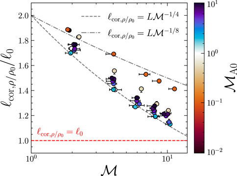
FIGURE 10. The correlation scale of ρ/ρ₀ for the supersonic experiments, relevant to our κ_‖ model, Eq. 41, as computed with Eq. 42, as a function of $\mathcal{M}$, colored in the same fashion as Figure 8. We show the driving scale, ℓ₀, with the red horizontal line. We annotate an upper and lower power law envelope, ${\ell }_{\text{cor},\rho /{\rho }_0}\propto {\mathcal{M}}^{-1/8}-{\mathcal{M}}^{-1/4}$, for the super-to-sub-Alfvénic experiments, respectively. In general, as $\mathcal{M}$ increases, the density fluctuations become correlated on smaller spatial scales, and the magnetic field suppresses the small-scale fluctuations.

Now we have all of the ingredients for estimating κ_‖ in a relevant astrophysical system. Because our model works in a ${\mathcal{M}}_{\text{A0}}\lesssim 1$ and $\mathcal{M}>1$ plasma state, we choose a typical, cold MC, where T ∼ 10 K (e.g., Wolfire et al., 1995), χ ∼ 10^–6 and [p − 1]/[2p] = 1/4 (see Section 1.2), $\mathcal{M}\sim 10$ on the cloud scale L ∼ 10 pc, (Schneider et al., 2013; Federrath et al., 2016; Orkisz et al., 2017; Beattie et al., 2019), and, for at least some MCs, ${\mathcal{M}}_{\text{A}}<1\Rightarrow {\mathcal{M}}_{\text{A0}}<1$ (Li et al., 2013; Federrath et al., 2016; Hu et al., 2019; Heyer et al., 2020; Hoang et al., 2021; Hwang et al., 2021; Beattie et al., 2022). We take ${\mathcal{M}}_{\text{A0}}=1$, which for $\mathcal{M}\sim 10$, implies that $v_{\text{A0}}=c_s\mathcal{M}\sim 2{\text{kms}}^{-1}$ for a $c_s={[k_{\text{B}}T/(\mu m_{\text{H}})]}^{1/2}\sim 0.2\text{km}{\text{s}}^{-1}$ for μ = 2.33 (H₂ + He composition), and k_B, the Boltzmann constant. This means $v_{\text{A0,ion}}=v_{\text{A0}}/\sqrt{\chi }=2\times 10^3\text{km}{\text{s}}^{-1}$. Using Eq. 27, we can estimate ${\sigma }_s^2=2.25$. Because we are considering $\mathcal{M}$ on L = 10 pc, we ought to think of the cloud as an isolated system, where the k modes of the turbulence above the cloud-scale are “removed”. This means that ℓ₀ = L, and therefore ${\ell }_{\text{cor},\rho /{\rho }_0}=1.2{\ell }_0=12\text{pc}$, as per Figure 10. Populating Eq. 41 with these typical parameter values for sub-Alfvénic, supersonic MCs, then we find the parallel macroscopic diffusion coefficient is

References

Abe, D., Inoue, T., Inutsuka, S.-i., and Matsumoto, T. (2020). Classification of Filament Formation Mechanisms in Magnetized Molecular Clouds. arXiv e-printsarXiv:2012.02205.
Ade, P. A. R., Aghanim, N., Alves, M. I. R., Arnaud, M., Arzoumanian, D., et al. (2016a). Planck Intermediate Results. XXXV. Probing the Role of the Magnetic Field in the Formation of Structure in Molecular Clouds. Astron. Astrophys. 586, A138. doi:10.1051/0004-6361/201525896
Aghanim, N., Alves, M. I. R., Arnaud, M., Arzoumanian, D., Aumont, J., et al. (2016b). Planck Intermediate Results. XXXIV. The Magnetic Field Structure in the Rosette Nebula. Astron. Astrophys. 586, A137. doi:10.1051/0004-6361/201525616
Armstrong, J. W., Rickett, B. J., and Spangler, S. R. (1995). Electron Density Power Spectrum in the Local Interstellar Medium. Astrophys. J. 443, 209. doi:10.1086/175515
Bai, X.-N. (2022). Toward First-Principles Characterization of Cosmic-Ray Transport Coefficients from Multiscale Kinetic Simulations. Astrophys. J. 928, 112. doi:10.3847/1538-4357/ac56e1
Barreto-Mota, L., de Gouveia Dal Pino, E. M., Burkhart, B., Melioli, C., Santos-Lima, R., and Kadowaki, L. H. S. (2021). Magnetic Field Orientation in Self-Gravitating Turbulent Molecular Clouds. arXiv e-printsarXiv:2101.03246.
Beattie, J. R., and Federrath, C. (2020). Filaments and Striations: Anisotropies in Observed, Supersonic, Highly Magnetized Turbulent Clouds. Mon. Not. R. Astron. Soc. 492, 668–685. doi:10.1093/mnras/stz3377
Beattie, J. R., Federrath, C., Klessen, R. S., and Schneider, N. (2019). The Relation Between the Turbulent Mach Number and Observed Fractal Dimensions of Turbulent Clouds. Mon. Not. R. Astron. Soc. 488, 2493–2502. doi:10.1093/mnras/stz1853
Beattie, J. R., Federrath, C., and Seta, A. (2020). Magnetic Field Fluctuations in Anisotropic, Supersonic Turbulence. Mon. Not. R. Astron. Soc. 498, 1593–1608. doi:10.1093/mnras/staa2257
Beattie, J. R., Krumholz, M. R., Skalidis, R., Federrath, C., Seta, A., Crocker, R. M., et al. (2022). Energy Balance and Alfv∖’En Mach Numbers in Compressible Magnetohydrodynamic Turbulence with a Large-Scale Magnetic Field. arXiv e-printsarXiv:2202.13020.
Beattie, J. R., Mocz, P., Federrath, C., and Klessen, R. S. (2021a). A Multishock Model for the Density Variance of Anisotropic, Highly Magnetized, Supersonic Turbulence. Mon. Not. R. Astron. Soc. 504, 4354–4368. doi:10.1093/mnras/stab1037
Beattie, J. R., Mocz, P., Federrath, C., and Klessen, R. S. (2021b). The Density Distribution and the Physical Origins of Density Intermittency in Sub- to Trans-Alfvenic Supersonic Turbulence. arXiv e-printsarXiv:2109.10470.
Beck, R., and Wielebinski, R. (2013). Magnetic Fields Galaxies 5641. doi:10.1007/978-94-007-5612-0∖_13
Bell, A. (2013). Cosmic Ray Acceleration. Astropart. PhysicsSeeing High-Energy Universe Cherenkov Telesc. Array - Sci. Explor. CTA 43, 56–70. doi:10.1016/j.astropartphys.2012.05.022
Boldyrev, S., and Perez, J. C. (2009). Spectrum of Weak Magnetohydrodynamic Turbulence. Phys. Rev. Lett. 103, 225001. doi:10.1103/PhysRevLett.103.225001
Boldyrev, S. (2006). Spectrum of Magnetohydrodynamic Turbulence. Phys. Rev. Lett. 96, 115002. doi:10.1103/PhysRevLett.96.115002
Bonne, L., Schneider, N., Bontemps, S., Clarke, S. D., Gusdorf, A., Lehmann, A., et al. (2020). Dense Gas Formation in the Musca Filament Due to the Dissipation of a Supersonic Converging Flow. Astron. Astrophys. 641, A17. doi:10.1051/0004-6361/201937104
Booth, C. M., Agertz, O., Kravtsov, A. V., and Gnedin, N. Y. (2013). Simulations of Disk Galaxies with Cosmic Ray Driven Galactic Winds. Astrophys. J. 777, L16. doi:10.1088/2041-8205/777/1/L16
Bouchut, F., Klingenberg, C., and Waagan, K. (2010). A Multiwave Approximate Riemann Solver for Ideal Mhd Based on Relaxation Ii: Numerical Implementation with 3 and 5 waves. Numer. Math. (Heidelb). 115, 647–679. doi:10.1007/s00211-010-0289-4
Boulares, A., and Cox, D. P. (1990). Galactic Hydrostatic Equilibrium with Magnetic Tension and Cosmic-Ray Diffusion. Astrophys. J. 365, 544. doi:10.1086/169509
Brunt, C. M., Federrath, C., and Price, D. J. (2010a). A Method for Reconstructing the PDF of a 3D Turbulent Density Field from 2D Observations. MNRAS 405, L56–L60. doi:10.1111/j.1745-3933.2010.00858.x
Brunt, C. M., Federrath, C., and Price, D. J. (2010b). A Method for Reconstructing the Variance of a 3d Physical Field from 2d Observations: Application to Turbulence in the Interstellar Medium. Mon. Not. R. Astron. Soc. 403, 1507–1515. doi:10.1111/j.1365-2966.2009.16215.x
Brunt, C. M., Heyer, M. H., and Mac Low, M. M. (2009). Turbulent Driving Scales in Molecular Clouds. Astron. Astrophys. 504, 883–890. doi:10.1051/0004-6361/200911797
Burgers, J. (1948). A Mathematical Model Illustrating the Theory of Turbulence. Adv. Appl. Mech. 1, 171–199. doi:10.1016/S0065-2156(08)70100-5
Burkhart, B., Falceta-Gonçalves, D., Kowal, G., and Lazarian, A. (2009). Density Studies of MHD Interstellar Turbulence: Statistical Moments, Correlations and Bispectrum. Astrophys. J. 693, 250–266. doi:10.1088/0004-637x/693/1/250
Burkhart, B. (2018). The Star Formation Rate in the Gravoturbulent Interstellar Medium. Astrophys. J. 863, 118. doi:10.3847/1538-4357/aad002
Bustard, C., and Zweibel, E. G. (2021). Cosmic-Ray Transport, Energy Loss, and Influence in the Multiphase Interstellar Medium. Astrophys. J. 913, 106. doi:10.3847/1538-4357/abf64c
Caprioli, D., Blasi, P., Amato, E., and Vietri, M. (2009). Dynamical Feedback of Self-Generated Magnetic Fields in Cosmic Ray Modified Shocks. Mon. Not. R. Astron. Soc. 395, 895–906. doi:10.1111/j.1365-2966.2009.14570.x
Chandrasekhar, S., and Fermi, E. (1953). Magnetic Fields In Spiral Arms. Astrophys. J. 118, 113. doi:10.1086/145731
Chen, C.-Y., and Ostriker, E. C. (2014). Formation of Magnetized Prestellar Cores with Ambipolar Diffusion and Turbulence. Astrophys. J. 785, 69. doi:10.1088/0004-637X/785/1/69
Chen, M. C.-Y., Francesco, J. D., Rosolowsky, E., Keown, J., Pineda, J. E., Friesen, R. K., et al. (2020). Velocity-Coherent Filaments in NGC 1333: Evidence for Accretion Flow? Astrophys. J. 891, 84. doi:10.3847/1538-4357/ab7378
Colling, C., Hennebelle, P., Geen, S., Iffrig, O., and Bournaud, F. (2018). Impact of Galactic Shear and Stellar Feedback on Star Formation. Astron. Astrophys. 620, A21. doi:10.1051/0004-6361/201833161
Cox, N. L. J., Arzoumanian, D., André, P., Rygl, K. L. J., Prusti, T., Men’shchikov, A., et al. (2016). Filamentary Structure and Magnetic Field Orientation in Musca. Astron. Astrophys. 590, A110. doi:10.1051/0004-6361/201527068
Crocker, R. M., Krumholz, M. R., and Thompson, T. A. (2021a). Cosmic Rays Across the Star-Forming Galaxy Sequence - I. Cosmic Ray Pressures and Calorimetry. Mon. Not. R. Astron. Soc. 502, 1312–1333. doi:10.1093/mnras/stab148
Crocker, R. M., Krumholz, M. R., and Thompson, T. A. (2021b). Cosmic Rays Across the Star-Forming Galaxy Sequence - II. Stability Limits and the Onset of Cosmic Ray-Driven Outflows. Mon. Not. R. Astron. Soc. 503, 2651–2664. doi:10.1093/mnras/stab502
Davis, L. (1951). The Strength of Interstellar Magnetic Fields. Phys. Rev. 81, 890–891. doi:10.1103/PhysRev.81.890.2
Dobbs, C. L., Burkert, A., and Pringle, J. E. (2011). Why are Most Molecular Clouds not Gravitationally Bound? Mon. Not. R. Astron. Soc. 413, 2935–2942. doi:10.1111/j.1365-2966.2011.18371.x
Dubey, A., Fisher, R., Graziani, C., Jordan, G. C., IVLamb, D. Q., Reid, L. B., et al. (2008). “Challenges of Extreme Computing Using the FLASH Code,”Numer. Model. Space Plasma Flows of. Editors N. V. Pogorelov, E. Audit, and G. P. Zank (San Franciso, CA, United States: Astronomical Society of the Pacific Conference Series), 385, 145.
Elmegreen, B. G. (2009). “Star Formation in Disks: Spiral Arms, Turbulence, and Triggering Mechanisms,”. Galaxy Disk Cosmol. Context of. Editors J. Andersen, B. m. Nordströara, and J. Bland -Hawthorn (Cambridge, United Kingdom: IAU Symposium), 254, 289–300. doi:10.1017/S1743921308027713
Falceta-Gonçalves, D., Kowal, G., Falgarone, E., and Chian, A. C.-L. (2014). Turbulence in the Interstellar Medium. Nonlinear process. geophys. 21, 587–604. doi:10.5194/npg-21-587-2014
Federrath, C., and Banerjee, S. (2015). The Density Structure and Star Formation Rate of Non-Isothermal Polytropic Turbulence. Mon. Not. R. Astron. Soc. 448, 3297–3313. doi:10.1093/mnras/stv180
Federrath, C. (2015). Inefficient Star Formation Through Turbulence, Magnetic Fields and Feedback. Mon. Not. R. Astron. Soc. 450, 4035–4042. doi:10.1093/mnras/stv941
Federrath, C., Klessen, R. S., Iapichino, L., and Beattie, J. R. (2021). The Sonic Scale of Interstellar Turbulence. Nat. Astron. 5, 365–371. doi:10.1038/s41550-020-01282-z
Federrath, C., and Klessen, R. S. (2013). On the Star Formation Efficiency of Turbulent Magnetized Clouds. Astrophys. J. 763, 51. doi:10.1088/0004-637X/763/1/51
Federrath, C., Klessen, R. S., and Schmidt, W. (2008). The Density Probability Distribution in Compressible Isothermal Turbulence: Solenoidal Versus Compressive Forcing. Astrophys. J. 688, L79–L82. doi:10.1086/595280
Federrath, C., Klessen, R. S., and Schmidt, W. (2009). The Fractal Density Structure in Supersonic Isothermal Turbulence: Solenoidal Versus Compressive Energy Injection. Astrophys. J. 692, 364–374. doi:10.1088/0004-637x/692/1/364
Federrath, C., and Klessen, R. S. (2012). The Star Formation Rate of Turbulent Magnetized Clouds: Comparing Theory, Simulations, and Observations. Astrophys. J., 156. doi:10.1088/0004-637X/761/2/156
Federrath, C. (2016). Magnetic Field Amplification in Turbulent Astrophysical Plasmas. J. Plasma Phys. 82, 535820601. doi:10.1017/S0022377816001069
Federrath, C., Rathborne, J. M., Longmore, S. N., Kruijssen, J. M. D., Bally, J., Contreras, Y., et al. (2017). “The Link Between Solenoidal Turbulence and Slow Star Formation in G0.253+0.016,”. Multi-Messenger Astrophysics Galactic Centre of. Editors R. M. Crocker, S. N. Longmore, and G. V. Bicknell (Cambridge, United Kingdom: IAU Symposium), 322, 123–128. doi:10.1017/S1743921316012357
Federrath, C., Rathborne, J. M., Longmore, S. N., Kruijssen, J. M. D., Bally, J., Contreras, Y., et al. (2016). The Link Between Turbulence, Magnetic Fields, Filaments, And Star Formation in the Central Molecular Zone Cloud G0.253+0.016. Astrophys. J. 832, 143. doi:10.3847/0004-637X/832/2/143
Federrath, C., Roman-Duval, J., Klessen, R., Schmidt, W., and Mac Low, M. M. (2010). Comparing the Statistics of Interstellar Turbulence in Simulations And Observations: Solenoidal Versus Compressive Turbulence Forcing. Astron. Astrophys. 512, A81. doi:10.1051/0004-6361/200912437
Federrath, C., Roman-Duval, J., Klessen, R. S., Schmidt, W., and Mac Low, M. M. (2022). TG: Turbulence Generator. Houghton, Michigan, United States: Astrophysics Source Code Library record ascl:2204.001.
Federrath, C., Sur, S., Schleicher, D. R. G., Banerjee, R., and Klessen, R. S. (2011). A New Jeans Resolution Criterion for (M)HD Simulations of Self-Gravitating Gas: Application to Magnetic Field Amplification by Gravity-Driven Turbulence. Astrophys. J. 731, 62. doi:10.1088/0004-637X/731/1/62
Ferrière, K. M. (2001). The Interstellar Environment of Our Galaxy. Rev. Mod. Phys. 73, 1031–1066. doi:10.1103/revmodphys.73.1031
Field, G. B., Goldsmith, D. W., and Habing, H. J. (1969). Cosmic-Ray Heating of the Interstellar Gas. Astrophys. J. 155, L149. doi:10.1086/180324
Foreman-Mackey, D., Hogg, D. W., Lang, D., and Goodman, J. (2013). Emcee: The Mcmc Hammer, 125. San Francisco, CA, United States: Publications of the Astronomical Society of the Pacific, 306.
Freedman, M. H., and He, Z.-X. (1991). Divergence-Free Fields: Energy and Asymptotic Crossing Number. Ann. Math. 134, 189–229. doi:10.2307/2944336
Fryxell, B., Olson, K., Ricker, P., Timmes, F. X., Zingale, M., Lamb, D. Q., et al. (2000). Flash: An Adaptive Mesh Hydrodynamics Code for Modeling Astrophysical Thermonuclear Flashes. Astrophys. J. Suppl. Ser. 131, 273–334. doi:10.1086/317361
Gaensler, B. M., Haverkorn, M., Burkhart, B., Newton-McGee, K. J., Ekers, R. D., Lazarian, A., et al. (2011). Low-Mach-Number Turbulence in Interstellar Gas Revealed by Radio Polarization Gradients. Nature 478, 214–217. doi:10.1038/nature10446
Girichidis, P., Naab, T., Walch, S., Hanasz, M., Mac Low, M.-M., Ostriker, J. P., et al. (2016). Launching Cosmic-Ray-Driven Outflows from the Magnetized Interstellar Medium. Astrophys. J. 816, L19. doi:10.3847/2041-8205/816/2/L19
Goldreich, P., and Sridhar, S. (1995). Toward a Theory of Interstellar Turbulence. 2: Strong Alfvenic Turbulence. Astrophys. J. 438, 763–775. doi:10.1086/175121
Grisdale, K., Agertz, O., Romeo, A. B., Renaud, F., and Read, J. I. (2017). The Impact oif Stellar Feedback on the Density and Velocity Structure of the Interstellar Medium. Mon. Not. R. Astron. Soc. 466, 1093–1110. doi:10.1093/mnras/stw3133
Harris, C. R., Millman, K. J., van der Walt, S. J., Gommers, R., Virtanen, P., Cournapeau, D., et al. (2020). Array Programming with Numpy. Nature 585, 357–362. doi:10.1038/s41586-020-2649-2
Hennebelle, P., and Falgarone, E. (2012). Turbulent Molecular Clouds. Astron. Astrophys. Rev. 20, 55. doi:10.1007/s00159-012-0055-y
Heyer, M., Soler, J. D., and Burkhart, B. (2020). The Relative Orientation Between the Magnetic Field and Gradients of Surface Brightness Within Thin Velocity Slices of 12CO And 13CO Emission from the Taurus Molecular Cloud. Mon. Not. R. Astron. Soc. 496, 4546–4564. doi:10.1093/mnras/staa1760
Higashi, S., Susa, H., and Chiaki, G. (2021). Amplification of Turbulence in Contracting Prestellar Cores in Primordial Minihalos. Astrophys. J. 915, 107. doi:10.3847/1538-4357/ac01c7
Hoang, T. D., Bich Ngoc, N., Diep, P. N., Tram, L. N., Hoang, T., Lim, W., et al. (2021). Studying Magnetic Fields and Dust in M17 using Polarized Thermal Dust Emission Observed by SOFIA/HAWC+. arXiv:2108.10045.
Hoef, J. M. V. (2012). Who Invented the Delta Method? Am. Statistician 66, 124–127. doi:10.1080/00031305.2012.687494
Hopkins, P. F. (2013). A Model for (non-lognormal) Density Distributions in Isothermal Turbulence. Mon. Not. R. Astron. Soc. 430, 1880–1891. doi:10.1093/mnras/stt010
Hopkins, P. F., Chan, T. K., Squire, J., Quataert, E., Ji, S., Kereš, D., et al. (2021). Effects of Different Cosmic Ray Transport Models on Galaxy Formation. Mon. Not. R. Astron. Soc. 501, 3663–3669. doi:10.1093/mnras/staa3692
Hu, Y., Lazarian, A., and Xu, S. (2022). Superdiffusion of cosmic Rays in Compressible Magnetized Turbulence. Mon. Not. R. Astron. Soc. 512, 2111–2124. doi:10.1093/mnras/stac319
Hu, Y., Yuen, K. H., Lazarian, V., Ho, K. W., Benjamin, R. A., Hill, A. S., et al. (2019). Magnetic Field Morphology in Interstellar Clouds with the Velocity Gradient Technique. Nat. Astron. 3, 776–782. doi:10.1038/s41550-019-0769-0
Hunter, J. D. (2007). Matplotlib: A 2d Graphics Environment. Comput. Sci. Eng. 9, 90–95. doi:10.1109/MCSE.2007.55
Hwang, J., Kim, J., Pattle, K., Kwon, W., Sadavoy, S., Koch, P. M., et al. (2021). The JCMT BISTRO Survey: The Distribution of Magnetic Field Strengths Toward the OMC-1 Region. Astrophys. J. 913, 85. doi:10.3847/1538-4357/abf3c4
Iroshnikov, P. S. (1964). Turbulence of a Conducting Fluid in a Strong Magnetic Field. Sov. Ast 7, 566.
Jaupart, E., and Chabrier, G. (2020). Evolution of the Density PDF in Star-Forming Clouds: The Role of Gravity. Astrophys. J. 903, L2. doi:10.3847/2041-8213/abbda8
Jin, K., Salim, D. M., Federrath, C., Tasker, E. J., Habe, A., and Kainulainen, J. T. (2017). On the Effective Turbulence Driving Mode of Molecular Clouds Formed in Disc Galaxies. Mon. Not. R. Astron. Soc. 469, 383–393. doi:10.1093/mnras/stx737
Karlsson, T., Bromm, V., and Bland-Hawthorn, J. (2013). Pregalactic Metal Enrichment: The Chemical Signatures of the First Stars. Rev. Mod. Phys. 85, 809–848. doi:10.1103/RevModPhys.85.809
Khullar, S., Federrath, C., Krumholz, M. R., and Matzner, C. D. (2021). The Density Structure of Supersonic Self-Gravitating Turbulence. arXiv e-printsarXiv:2107.00725.
Kim, J., and Ryu, D. (2005). Density Power Spectrum of Compressible Hydrodynamic Turbulent Flows. Astrophys. J. 630, L45–L48. doi:10.1086/491600
Kitsionas, S., Federrath, C., Klessen, R. S., Schmidt, W., Price, D. J., Dursi, L. J., et al. (2009). Algorithmic Comparisons of Decaying, Isothermal, Supersonic Turbulence. Astron. Astrophys. 508, 541–560. doi:10.1051/0004-6361/200811170
Kolmogorov, A. N. (1941). The Local Structure of Turbulence in Incompressible Viscous Fluid for Very Large Reynolds Numbers. Dokl. Akad. Nauk. Sssr 30, 301–305. doi:10.1098/rspa.1991.0075
Konstandin, L., Federrath, C., Klessen, R. S., and Schmidt, W. (2012a). Statistical Properties of Supersonic Turbulence in the Lagrangian and Eulerian Frameworks. J. Fluid Mech. 692, 183–206. doi:10.1017/jfm.2011.503
Konstandin, L., Girichidis, P., Federrath, C., and Klessen, R. S. (2012b). A New Density Variance-Mach Number Relation for Subsonic and Supersonic Isothermal Turbulence. Astrophys. J. 761, 149. doi:10.1088/0004-637X/761/2/149
Körtgen, B., Federrath, C., and Banerjee, R. (2017). The Driving Of Turbulence in Simulations of Molecular Cloud Formation and Evolution. Mon. Not. R. Astron. Soc. 472, 2496–2503. doi:10.1093/mnras/stx2208
Körtgen, B., and Soler, J. D. (2020). The Relative Orientation Between the Magnetic Field and Gas Density Structures in Non-Gravitating Turbulent Media. Mon. Not. R. Astron. Soc. 499, 4785–4792. doi:10.1093/mnras/staa3078
Kraichnan, R. H. (1965). Inertial-Range Spectrum of Hydromagnetic Turbulence. Phys. Fluids (1994). 8, 1385–1387. doi:10.1063/1.1761412
Kritsuk, A. G., Ustyugov, S. D., and Norman, M. L. (2017). The Structure and Statistics of Interstellar Turbulence. New J. Phys. 19, 065003. doi:10.1088/1367-2630/aa7156
Krumholz, M. R., and Burkhart, B. (2016). Is Turbulence in the Interstellar Medium Driven by Feedback or Gravity? an Observational Test. Mon. Not. R. Astron. Soc. 458, 1671–1677. doi:10.1093/mnras/stw434
Krumholz, M. R., Crocker, R. M., Xu, S., Lazarian, A., Rosevear, M. T., and Bedwell-Wilson, J. (2020). Cosmic Ray Transport in Starburst Galaxies. Mon. Not. R. Astron. Soc. 493, 2817–2833. doi:10.1093/mnras/staa493
Krumholz, M. R., and Ting, Y.-S. (2018). Metallicity Fluctuation Statistics in the Interstellar Medium and Young Stars - I. Variance and Correlation. Mon. Not. R. Astron. Soc. 475, 2236–2252. doi:10.1093/mnras/stx3286
Kulsrud, R., and Pearce, W. P. (1969). The Effect of Wave-Particle Interactions on the Propagation of Cosmic Rays. Astrophys. J. 156, 445. doi:10.1086/149981
Lazarian, A., and Yan, H. (2014). Superdiffusion of Cosmic Rays: Implications for Cosmic Ray Acceleration. Astrophys. J. 784, 38. doi:10.1088/0004-637X/784/1/38
Lerche, I. (1967). Unstable Magnetosonic Waves in a Relativistic Plasma. Astrophys. J. 147, 689. doi:10.1086/149045
Li, H.-b., Fang, M., Henning, T., and Kainulainen, J. (2013). The Link Between Magnetic Fields and Filamentary Clouds: Bimodal Cloud Orientations in the Gould Belt. Mon. Not. R. Astron. Soc. 436, 3707–3719. doi:10.1093/mnras/stt1849
Li, H.-B., and Henning, T. (2011). The Alignment of Molecular Cloud Magnetic Fields with the Spiral Arms in M33. Nature 479, 499–501. doi:10.1038/nature10551
Li, H. B., Goodman, A., Sridharan, T. K., Houde, M., Li, Z. Y., Novak, G., et al. (2014). “The Link Between Magnetic Fields and Cloud/Star Formation,” in Protostars and planets VI. Editors H. Beuther, R. S. Klessen, C. P. Dullemond, and T. Henning., 101. doi:10.2458/azu_uapress_9780816531240-ch005
Lithwick, Y., and Goldreich, P. (2001). Compressible Magnetohydrodynamic Turbulence in Interstellar Plasmas. Astrophys. J. 562, 279–296. doi:10.1086/323470
Litvinenko, Y. E., and Effenberger, F. (2014). Analytical Solutions of a Fractional Diffusion-Advection Equation for Solar Cosmic-Ray Transport. Astrophys. J. 796, 125. doi:10.1088/0004-637X/796/2/125
Liu, J., Qiu, K., and Zhang, Q. (2021). Magnetic Fields in Star Formation: A Complete Compilation of All the DCF Estimations. arXiv e-printsarXiv:2111.05836.
Lu, Z.-J., Pelkonen, V.-M., Padoan, P., Pan, L., Haugbølle, T., and Nordlund, Å. (2020). The Effect of Supernovae on the Turbulence and Dispersal of Molecular Clouds. arXiv e-printsarXiv:2007.09518.
Malinen, J., Montier, L., Montillaud, J., Juvela, M., Ristorcelli, I., Clark, S. E., et al. (2016). Matching Dust Emission Structures and Magnetic Field in High-Latitude Cloud L1642: Comparing Herschel and Planck Maps. Mon. Not. R. Astron. Soc. 460, 1934–1945. doi:10.1093/mnras/stw1061
Marchal, A., and Miville-Deschênes, M.-A. (2021). Thermal and Turbulent Properties of the Warm Neutral Medium in the Solar Neighborhood. Astrophys. J. 908, 186. doi:10.3847/1538-4357/abd108
Marder, B. (1987). A Method for Incorporating Gauss’ Law into Electromagnetic Pic Codes. J. Comput. Phys. 68, 48–55. doi:10.1016/0021-9991(87)90043-X
McKee, C. F., Stacy, A., and Li, P. S. (2020). Magnetic Fields in the Formation of the First Stars - I. Theory Versus Simulation. Mon. Not. R. Astron. Soc. 496, 5528–5551. doi:10.1093/mnras/staa1903
Menon, S. H., Federrath, C., and Kuiper, R. (2020). On the Turbulence Driving Mode of Expanding H II Regions. Mon. Not. R. Astron. Soc. 493, 4643–4656. doi:10.1093/mnras/staa580
Mocz, P., and Burkhart, B. (2019). A Markov Model for Non-Lognormal Density Distributions in Compressive Isothermal Turbulence. Astrophys. J. 884, L35. doi:10.3847/2041-8213/ab48f6
Mocz, P., and Burkhart, B. (2018). Star Formation from Dense Shocked Regions in Supersonic Isothermal Magnetoturbulence. Mon. Not. R. Astron. Soc. 480, 3916–3927. doi:10.1093/mnras/sty1976
Mohapatra, R., Federrath, C., and Sharma, P. (2020a). Turbulence in Stratified Atmospheres: Implications for the Intracluster Medium. Mon. Not. R. Astron. Soc. 493, 5838–5853. doi:10.1093/mnras/staa711
Mohapatra, R., Federrath, C., and Sharma, P. (2020b). Turbulent Density and Pressure Fluctuations in the Stratified Intracluster Medium. arXiv e-printsarXiv:2010.12602.
Molina, F. Z., Glover, S. C. O., Federrath, C., and Klessen, R. S. (2012). The Density Variance–Mach Number Relation in Supersonic Turbulence – I. Isothermal, Magnetized Gas. Mon. Not. R. Astron. Soc. 423, 2680–2689. doi:10.1111/j.1365-2966.2012.21075.x
Nolan, C. A., Federrath, C., and Sutherland, R. S. (2015). The Density Variance-Mach Number Relation in Isothermal and Non-Isothermal Adiabatic Turbulence. Mon. Not. R. Astron. Soc. 451, 1380–1389. doi:10.1093/mnras/stv1030
Omukai, K., Tsuribe, T., Schneider, R., and Ferrara, A. (2005). Thermal and Fragmentation Properties of Star-Forming Clouds in Low-Metallicity Environments. Astrophys. J. 626, 627–643. doi:10.1086/429955
Orkisz, J. H., Pety, J., Gerin, M., Bron, E., Guzmán, V. V., Bardeau, S., et al. (2017). Turbulence and Star Formation Efficiency in Molecular Clouds: Solenoidal Versus Compressive Motions in Orion B. Astron. Astrophys. 599, A99. doi:10.1051/0004-6361/201629220
Oughton, S., and Matthaeus, W. H. (2020). Critical Balance and the Physics of Magnetohydrodynamic Turbulence. Astrophys. J. 897, 37. doi:10.3847/1538-4357/ab8f2a
Oughton, S., Priest, E. R., and Matthaeus, W. H. (1994). The Influence of a Mean Magnetic Field on Three-Dimensional Magnetohydrodynamic Turbulence. J. Fluid Mech. 280, 95–117. doi:10.1017/S0022112094002867
Owen, E. R., On, A. Y. L., Lai, S.-P., and Wu, K. (2021). Observational Signatures of Cosmic-Ray Interactions in Molecular Clouds. Astrophys. J. 913, 52. doi:10.3847/1538-4357/abee1a
Padoan, P., Nordlund, P., and Jones, B. J. T. (1997). Universality of the Stellar Initial Mass Function. Commmunications Konkoly Observatory Hung. 100, 341–362.
Padoan, P., and Nordlund, Å. (1999). A Super-Alfvénic Model of Dark Clouds. Astrophys. J. 526, 279–294. doi:10.1086/307956
Padoan, P., and Nordlund, Å. (2011). The Star Formation Rate of Supersonic Magnetohydrodynamic Turbulence. Astrophys. J. 730, 40. doi:10.1088/0004-637X/730/1/40
Passot, T., and Vázquez-Semadeni, E. (1998). Density Probability Distribution in One-Dimensional Polytropic Gas Dynamics. Phys. Rev. E 58, 4501–4510. doi:10.1103/PhysRevE.58.4501
Pedaletti, G., Torres, D. F., Gabici, S., de Oña Wilhelmi, E., Mazin, D., and Stamatescu, V. (2013). On the Potential of the Cherenkov Telescope Array for the Study of Cosmic-Ray Diffusion in Molecular Clouds. Astron. Astrophys. 550, A123. doi:10.1051/0004-6361/201220583
Perez, J. C., and Boldyrev, S. (2008). On Weak and Strong Magnetohydrodynamic Turbulence. Astrophys. J. 672, L61–L64. doi:10.1086/526342
Pillai, T. G. S., Clemens, D. P., Reissl, S., Myers, P. C., Kauffmann, J., Lopez-Rodriguez, E., et al. (2020). Magnetized Filamentary Gas Flows Feeding the Young Embedded Cluster in Serpens South. Nat. Astron. 4, 1195–1201. doi:10.1038/s41550-020-1172-6
Plotnikov, I., Ostriker, E. C., and Bai, X.-N. (2021). Influence of Ion-Neutral Damping on the Cosmic-Ray Streaming Instability: Magnetohydrodynamic Particle-in-Cell Simulations. Astrophys. J. 914, 3. doi:10.3847/1538-4357/abf7b3
Price, D. J., and Federrath, C. (2010). A Comparison Between Grid And Particle Methods on the Statistics of Driven, Supersonic, Isothermal Turbulence. Mon. Not. R. Astron. Soc. 406, 1659–1674. doi:10.1111/j.1365-2966.2010.16810.x
Price, D. J., Federrath, C., and Brunt, C. M. (2011). The Density Variance-Mach Number Relation in Supersonic, Isothermal Turbulence. Astrophys. J. 727, L21–L1389. doi:10.1088/2041-8205/727/1/L21
Rathborne, J. M., Longmore, S. N., Jackson, J. M., Alves, J. F., Bally, J., Bastian, N., et al. (2015). A Cluster in the Making: ALMA Reveals the Initial Conditions for High-Mass Cluster Formation. Astrophys. J. 802, 125. doi:10.1088/0004-637X/802/2/125
Richardson, L. F. (1926). Atmospheric Diffusion Shown on a Distance-Neighbour Graph. Proc. R. Soc. Lond. Ser. A 110, 709–737. doi:10.1098/rspa.1926.0043
Robertson, B., and Goldreich, P. (2018). Dense Regions in Supersonic Isothermal Turbulence. Astrophys. J. 854, 88. doi:10.3847/1538-4357/aaa89e
Salem, M., Bryan, G. L., and Hummels, C. (2014). Cosmological Simulations of Galaxy Formation with Cosmic Rays. Astrophys. J. 797, L18. doi:10.1088/2041-8205/797/2/L18
Sampson, M. L., Beattie, J. R., Krumholz, M. R., Crocker, R. M., Federrath, C., and Seta, A. (2022). Turbulent Diffusion of Streaming Cosmic Rays in Compressible, Partially Ionised Plasma. arXiv e-printsarXiv:2205.08174.
Scannapieco, E., and Safarzadeh, M. (2018). Modeling Star Formation as a Markov Process in a Supersonic Gravoturbulent Medium. Astrophys. J. 865, L14. doi:10.3847/2041-8213/aae1f9
Schekochihin, A. A., Cowley, S. C., Dorland, W., Hammett, G. W., Howes, G. G., Quataert, E., et al. (2009). Astrophysical Gyrokinetics: Kinetic and Fluid Turbulent Cascades in Magnetized Weakly Collisional Plasmas. Astrophys. J. Suppl. Ser. 182, 310–377. doi:10.1088/0067-0049/182/1/310
Schekochihin, A. A., Cowley, S. C., Taylor, S. F., Maron, J. L., and McWilliams, J. C. (2004). Simulations of the Small-Scale Turbulent Dynamo. Astrophys. J. 612, 276–307. doi:10.1086/422547
Schekochihin, A. A., and Cowley, S. C. (2007). “Turbulence and Magnetic Fields in Astrophysical Plasmas,” in Magnetohydrodynamics: Historical evolution and Trends. Editors S. Molokov, R. Moreau, and H. K. Moffatt, 85.
Schneider, N., André, P., Könyves, V., Bontemps, S., Motte, F., Federrath, C., et al. (2013). What Determines the Density Structure of Molecular Clouds? A Case Study of Orion B with Herschel. Astrophys. J. 766, L17. doi:10.1088/2041-8205/766/2/L17
Schruba, A., Kruijssen, J. M. D., and Leroy, A. K. (2019). How Galactic Environment Affects the Dynamical State of Molecular Clouds and their Star Formation Efficiency. Astrophys. J. 883, 2. doi:10.3847/1538-4357/ab3a43
Seifried, D., Walch, S., Weis, M., Reissl, S., Soler, J. D., Klessen, R. S., et al. (2020). From Parallel to Perpendicular – on the Orientation of Magnetic Fields in Molecular Clouds. arXiv e-printsarXiv:2003.00017.
Seligman, D. Z., Rogers, L. A., Feinstein, A. D., Krumholz, M. R., Beattie, J. R., Federrath, C., et al. (2022). Theoretical and Observational Evidence for Coriolis Effects in Coronal Magnetic Fields Via Direct Current Driven Flaring Events. arXiv e-printsarXiv:2201.03697.
Seta, A., and Beck, R. (2019). Revisiting the Equipartition Assumption in Star-Forming Galaxies. Galaxies 7, 45. doi:10.3390/galaxies7020045
Seta, A., and Federrath, C. (2021a). Magnetic Fields in the Milky Way from Pulsar Observations: Effect of the Correlation Between Thermal Electrons and Magnetic Fields. Mon. Not. R. Astron. Soc. 502, 2220–2237. doi:10.1093/mnras/stab128
Seta, A., and Federrath, C. (2021b). Saturation Mechanism of the Fluctuation Dynamo in Supersonic Turbulent Plasmas. Phys. Rev. Fluids 6, 103701. doi:10.1103/physrevfluids.6.103701
Seta, A., and Federrath, C. (2022). Turbulent Dynamo in the Two-Phase Interstellar Medium. arXiv e-printsarXiv:2202.08324.
Sharda, P., Menon, S. H., Federrath, C., Krumholz, M. R., Beattie, J. R., Jameson, K. E., et al. (2021). First Extragalactic Measurement of the Turbulence Driving Parameter: ALMA Observations of the Star-Forming Region N159E in the Large Magellanic Cloud. Mon. Not. R. Astron. Soc. doi:10.1093/mnras/stab3048
Skalidis, R., Sternberg, J., Beattie, J. R., Pavlidou, V., and Tassis, K. (2021a). Why Take the Square Root? an Assessment of Interstellar Magnetic Field Strength Estimation Methods. arXiv e-printsarXiv:2109.10925.
Skalidis, R., and Tassis, K. (2020). High-Accuracy Estimation of Magnetic Field Strength in the Interstellar Medium from Dust Polarization. arXiv e-printsarXiv:2010.15141.
Skalidis, R., Tassis, K., Panopoulou, G. V., Pineda, J. L., Gong, Y., Mandarakas, N., et al. (2021b). HI-H2 Transition: Exploring the Role of the Magnetic Field. arXiv e-printsarXiv:2110.11878.
Skilling, J. (1971). Cosmic Rays in the Galaxy: Convection or Diffusion? Astrophys. J. 170, 265. doi:10.1086/151210
Soler, J. D., Ade, P. A. R., Angilè, F. E., Ashton, P., Benton, S. J., Devlin, M. J., et al. (2017). The Relation Between the Column Density Structures and the Magnetic Field Orientation in the Vela C Molecular Complex. Astron. Astrophys. 603, A64. doi:10.1051/0004-6361/201730608
Soler, J. D., Hennebelle, P., Martin, P. G., Miville-Deschênes, M. A., Netterfield, C. B., and Fissel, L. M. (2013). An Imprint of Molecular Cloud Magnetization in the Morphology of the Dust Polarized Emission. Astrophys. J. 774, 128. doi:10.1088/0004-637X/774/2/128
Soler, J. D., and Hennebelle, P. (2017). What are we Learning from the Relative Orientation Between Density Structures and the Magnetic Field in Molecular Clouds? Astron. Astrophys. 607, A2. doi:10.1051/0004-6361/201731049
Squire, J., and Hopkins, P. F. (2017). The Distribution of Density in Supersonic Turbulence. Mon. Not. R. Astron. Soc. 471, 3753–3767. doi:10.1093/mnras/stx1817
Sridhar, S., and Goldreich, P. (1994). Toward a theory of Interstellar Turbulence. 1: Weak Alfvenic Turbulence. Astrophys. J. 432, 612. doi:10.1086/174600
Stewart, M., and Federrath, C. (2022). A New Method for Measuring the 3D Turbulent Velocity Dispersion of Molecular Clouds. Mon. Not. R. Astron. Soc. 509, 5237–5252. doi:10.1093/mnras/stab3313
Subramanian, K. (2019). From Primordial Seed Magnetic Fields to the Galactic Dynamo. Galaxies 7, 47. doi:10.3390/galaxies7020047
Subramanian, K. (2016). The Origin, Evolution and Signatures of Primordial Magnetic Fields. Rep. Prog. Phys. 79, 076901. doi:10.1088/0034-4885/79/7/076901
Tress, R. G., Smith, R. J., Sormani, M. C., Glover, S. C. O., Klessen, R. S., Mac Low, M.-M., et al. (2020). Simulations of the Star-Forming Molecular Gas in an Interacting M51-Like Galaxy. Mon. Not. R. Astron. Soc. 492, 2973–2995. doi:10.1093/mnras/stz3600
Tritsis, A., Federrath, C., Schneider, N., and Tassis, K. (2018). A New Method for Probing Magnetic Field Strengths from Striations in the Interstellar Medium. Mon. Not. R. Astron. Soc. 481, 5275–5285. doi:10.1093/mnras/sty2677
Tritsis, A., Panopoulou, G. V., Mouschovias, T. C., Tassis, K., and Pavlidou, V. (2015). Magnetic Field-Gas Density Relation and Observational Implications Revisited. Mon. Not. R. Astron. Soc. 451, 4384–4396. doi:10.1093/mnras/stv1133
Tritsis, A., and Tassis, K. (2018). Magnetic Seismology of Interstellar Gas Clouds: Unveiling a Hidden Dimension. Science 360, 635–638. doi:10.1126/science.aao1185
Tritsis, A., and Tassis, K. (2016). Striations in Molecular Clouds: Streamers or MHD Waves? Mon. Not. R. Astron. Soc. 462, 3602–3615. doi:10.1093/mnras/stw1881
Uhlig, M., Pfrommer, C., Sharma, M., Nath, B. B., Enßlin, T. A., and Springel, V. (2012). Galactic Winds Driven by Cosmic Ray Streaming. Mon. Not. R. Astron. Soc. 423, 2374–2396. doi:10.1111/j.1365-2966.2012.21045.x
Vazquez-Semadeni, E. (1994). Hierarchical Structure in Nearly Pressureless Flows as a Consequence of Self-Similar Statistics. Astrophys. J. 423, 681. doi:10.1086/173847
Virtanen, P., Gommers, R., Oliphant, T. E., Haberland, M., Reddy, T., Cournapeau, D., et al. (2020). SciPy 1.0: Fundamental Algorithms for Scientific Computing in Python. Nat. Methods 17, 261–272. doi:10.1038/s41592-019-0686-2
Waagan, K., Federrath, C., and Klingenberg, C. (2011). A Robust Numerical Scheme for Highly Compressible Magnetohydrodynamics: Nonlinear Stability, Implementation and Tests. J. Comput. Phys. 230, 3331–3351. doi:10.1016/j.jcp.2011.01.026
Wang, Y., Boldyrev, S., and Perez, J. C. (2011). Residual Energy in Magnetohydrodynamic Turbulence. Astrophys. J. 740, L36. doi:10.1088/2041-8205/740/2/L36
Wentzel, D. G. (1969). The Propagation and Anisotropy of Cosmic Rays. I. Theory for Steady Streaming. Astrophys. J. 156, 303. doi:10.1086/149965
Wolfire, M. G., Hollenbach, D., McKee, C. F., Tielens, A. G. G. M., and Bakes, E. L. O. (1995). The Neutral Atomic Phases of the Interstellar Medium. Astrophys. J. 443, 152. doi:10.1086/175510
Wolfire, M. G., McKee, C. F., Hollenbach, D., and Tielens, A. G. G. M. (2003). Neutral Atomic Phases of the Interstellar Medium in the Galaxy. Astrophys. J. 587, 278–311. doi:10.1086/368016
Xu, S., and Lazarian, A. (2021a). Cosmic Ray Streaming in the Turbulent Interstellar Medium. arXiv e-printsarXiv:2112.06941.
Xu, S., and Lazarian, A. (2022). Cosmic Ray Streaming in the Turbulent Interstellar Medium. Astrophys. J. 927, 94. doi:10.3847/1538-4357/ac4dfd
Xu, S., and Lazarian, A. (2021b). Small-Scale Turbulent Dynamo in Astrophysical Environments: Nonlinear Dynamo and Dynamo in a Partially Ionized Plasma. arXiv e-printsarXiv:2106.12598.
Xu, S., and Lazarian, A. (2016). Turbulent Dynamo in a Conducting Fluid and a Partially Ionized Gas. Astrophys. J. 833, 215. doi:10.3847/1538-4357/833/2/215
Xu, S., and Yan, H. (2013). Cosmic-Ray Parallel and Perpendicular Transport in Turbulent Magnetic Fields. Astrophys. J. 779, 140. doi:10.1088/0004-637X/779/2/140
Yang, L. P., Li, H., Li, S. T., Zhang, L., He, J. S., and Feng, X. S. (2019). Energy Occupationo of Waves and Structures in 3D Compressive MHD Turbulence. Mon. Not. R. Astron. Soc. 488, 859–867. doi:10.1093/mnras/stz1747
Yoon, H., Cho, J., and Kim, J. (2016). Density-Magnetic Field Correlation in Magnetohydrodynamic Turbulence Driven by Different Driving Schemes with Different Correlation Times. Astrophys. J. 831, 85. doi:10.3847/0004-637X/831/1/85
Keywords: magnetic fields, multi-phase interstellar medium, galaxies, cosmic rays, magnetohydrodynamic turbulence
Citation: Beattie JR, Krumholz MR, Federrath C, Sampson ML and Crocker RM (2022) Ion alfvén velocity fluctuations and implications for the diffusion of streaming cosmic rays. Front. Astron. Space Sci. 9:900900. doi: 10.3389/fspas.2022.900900
Received: 21 March 2022; Accepted: 06 June 2022;
Published: 06 October 2022.
Edited by:
Siyao Xu, Institute for Advanced Study, United StatesReviewed by:
Jonathan Squire, University of Otago, New ZealandXuening Bai, Tsinghua University, China
Copyright © 2022 Beattie, Krumholz, Federrath, Sampson and Crocker. This is an open-access article distributed under the terms of the Creative Commons Attribution License (CC BY). The use, distribution or reproduction in other forums is permitted, provided the original author(s) and the copyright owner(s) are credited and that the original publication in this journal is cited, in accordance with accepted academic practice. No use, distribution or reproduction is permitted which does not comply with these terms.
*Correspondence: James R. Beattie, james.beattie@anu.edu.au