PC index as a ground-based indicator of the solar wind energy incoming into the magnetosphere: (1) relation of PC index to the solar wind electric field E_KL

Highlights

The polar cap magnetic activity (estimated by the PC index) is controlled by the solar wind electric field E_KL affecting the magnetosphere.

The PC index responds to the E_KL influence through the field-aligned current (FAC) systems generated in the magnetosphere.

The PC index behavior certifies development and intensity of the magnetospheric disturbances.

The PC index can be used to validate the solar wind parameters measured by distant solar wind monitor.

1 Introduction

The PC index has been introduced as a value of the polar cap magnetic activity produced by the solar wind impact on the magnetosphere (Troshichev and Andrezen, 1985). Subsequent researches have demonstrated the high efficiency of such approach and the PC index was approved by International Association of Geomagnetism and Aeronomy (IAGA) as “a proxy for energy that enters into the magnetosphere during solar wind-magnetosphere coupling” (IAGA Resolutions, 2013; IAGA Resolution, 2021). This verdict was based on two fundamental features of the index: 1) PC index strongly follows variations of such solar wind characteristic, as electric field E_KL determining the state of magnetosphere, and 2) the PC index behavior predetermines development of the magnetosphere disturbances. This paper summarizes the issues concerning the PC index relation to the solar wind parameters and mechanisms of their influence on the magnetosphere: physical backgrounds and concept of PC index, method of the PC index derivation, relationship between the PC index and the solar wind electric field (E_KL), relation of the PC index to the solar wind dynamic pressure pulses (Pdyn), and other experimental results indicative of the PC index as an adequate ground-based indicator of the solar wind influence on the magnetosphere. The PC index treatment has displayed some unresolved or contradictory ideas on solar wind–magnetosphere coupling, which are also discussed in the paper, such as: mechanisms providing the link between the PC index and the solar wind electric field (E_KL), factors controlling delay in response of PC index to the E_KL field alterations, inconsistency between the PC index and E_KL field in particular cases, cross polar cap voltage, seasonal variations of the PC index and reasons of occasional difference between the PC values in the northern polar and southern polar caps. Relationships between the PC index and magnetospheric disturbances (magnetic storms and substroms) will be examined in separated paper.

2 Physical backgrounds

Nagata and Kokubun (1962) were the first who examined, under the name “daily quiet polar variation” (S^p _q), the magnetic activity typical of polar cap in periods free of magnetic disturbances in the auroral zone. Subsequently these variations were studied (Obayashi, 1967; Nishida, 1968a; Nishida, 1968b; Nishida and Maezawa, 1971) under the name of DP2 to distinguish them from magnetic substorms termed as DP1 (Akasofu, 1968). The DP2 current system consists of two current vortices with the sunward directed currents in the near-pole region but without any electrojet signatures in the auroral zone, the current intensity being controlled by the vertical southward (B_ZS) component of interplanetary magnetic field (IMF) (Nishida, 1968b). It was revealed later (Troshichev, 1975) that DP2 current vortices are terminated by geomagnetic latitudes Φ = 50–60.

Besides of the DP2 magnetic activity, related to southward IMF, there was found abnormal “near-pole DP variation”, related to northward IMF (Iwasaki, 1971; Maezawa, 1976; Kuznetsov and Troshichev, 1977), and magnetic variation “DPY”, related to azimuthal IMF B_Y component (Svalgaard, 1968; Mansurov, 1969; Matsushita et al., 1973; Friis-Christensen and Wilhjelm, 1975). Equivalent current systems of these disturbances were denoted, correspondingly, as DP3 and DP4 systems (Kuznetsov and Troshichev, 1977). The DP3 system consists of two current cells with opposite currents, observed in the limited near-pole region on the background of DP2 system. The DP4 current system includes currents flowing roughly along the geomagnetic latitudes in the day-time cusp region (Φ∼80°C); the current direction, defined by the By polarity, being opposite in the northern and southern polar caps.

Availability of the independent DP2 (b), DP3 (c) and DP4 (d) current systems related to southward, northward and azimuthal IMF components has been verified (Figure 1) by multi-functional analysis of relationships between the IMF components and the polar cap magnetic disturbances (Troshichev and Tsyganenko, 1979). Besides, the residual magnetic disturbance current system DP0, unrelated to the IMF (Figure 1A), was identified. The DP0 system is similar to DP2 system, but exists permanently, in particular, under condition of zero B_Z IMF. As it was shown later (Sergeev and Kuznetsov, 1981), the DP0 currents intensity correlates with the solar wind velocity (Vsw)². Results of analyses of the polar cap magnetic activity (Kuznetsov and Troshichev, 1977; Troshichev and Tsyganenko, 1979) occurred to be in good agreement with data of direct measurements of the electric field structure and intensity in polar cap fulfilled at satellites and in balloon experiments (Frank and Garnett, 1971; Heppner et al., 1971; Mozer et al., 1974). It was suggested (Troshichev et al., 1979a) that the polar cap magnetic activity can serve as a signature of substorm development.

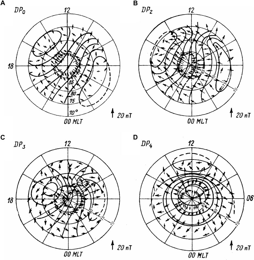
FIGURE 1. Current systems of the polar cap magnetic disturbances in summer season: (A) primary system DP0 independent on IMF (B) DP2 system related to southward B_ZS, (C) DP3 system related to northward B_ZN, (D) DP4 system related to azimuthal B_Y. Short arrows present distribution of the magnetic disturbances vectors on the ground surface. (Troshichev and Tsyganenko, 1979).

Results of magnetic measurements on board spacecrafts (Armstrong and Zmuda, 1970; Zmuda and Armstrong, 1974; Iijima and Potemra, 1976a; Iijima and Potemra, 1976b) revealed existence of planetary systems of electric currents flowing along geomagnetic field lines. The main system of field-aligned currents (FAC system), providing the solar wind–magnetosphere coupling, is the Region 1 system, which is observed permanently in the polar region. The R1 FAC system includes a layer of currents flowing into ionosphere on the dawn poleward boundary of the auroral oval and flowing out of ionosphere on the dusk poleward boundary of the oval, the current intensity being dependent on the IMF B_Z component orientation (Zmuda and Armstrong, 1974; Langel, 1975; Iijima and Potemra, 1976a; Iijima and Potemra, 1976b; Iijima and Potemra, 1982; Bythrow and Potemra, 1983).

The specific field-aligned current system, denoted as NBZ FAC, is observed in the sunlit near-pole area at latitudes of Φ > 75 under conditions of strong IMF northward B_ZN component (McDiarmid et al., 1977; McDiarmid et al., 1979; Iijima et al., 1984; Zanetti et al., 1984; Iijima and Shibaji, 1987). Polarity of these NBZ currents is opposite to the R1 FAC polarity: they flow into the ionosphere in the post-noon sector and flow out of the ionosphere in the pre-noon sector. The azimuthal IMF B_Y component generates the BY FAC system consisting of two current sheets (Wilhjelm et al., 1978), one of which is located on the equatorward side of the cusp, i.e., in Region 1, whereas other sheet is located on the poleward boundary boundary of the cusp. Direction of the field-aligned currents, determined by sign of the IMF B_Y component (Iijima et al., 1978; McDiarmid et al., 1978; McDiarmid et al., 1979; Saflekos and Potemra, 1980), is opposite in the northern and southern polar caps. Since the NBZ and B_Y field-aligned currents are closed through the day-time area of polar region, their intensity is maximum in the sunlit summer polar cap and is negligible in the winter polar cap.

Increase of particle precipitation in the auroral zone during substorm leads to formation of the R2 FAC system on the equatorial side of auroral oval, the R1 and R2 currents being outlined by poleward and equatorward boundaries of the oval (Zmuda and Armstrong, 1974; Iijiima and Potemra, 1976a). The R1/R2 FAC patterns (Iijima and Potemra, 1976a) were mapped to the equatorial plane by (Potemra, 1978), with use of the Fairfield and Mead (1975) model of magnetosphere, and by Antonova et al. (2006), with application of the “short” and advanced “long” magnetosphere models of Tsyganenko (1996), Tsyganenko (2002). In spite of essential difference of models, the results have demonstrated that both R1 and R2 field-aligned currents are mapped at the inner magnetospheric regions and do not related to the magnetosphere low-latitude boundary layer. The same conclusion was made by Ohtani et al. (1995) basing on results of simultaneous prenoon and postnoon FAC observations on board the Viking and DMSP-F7 satellites and by Chan and Russel (2000) when analyzing the data on field-aligned currents measured by ISEE 1 and 2 satellites at altitudes 2–9 R_E. According to studies (Antonova et al., 2013; Antonova et al., 2014; Antonova et al., 2018), the auroral oval is related to plasma ring surrounding the Earth at geocentric distances ∼7–10 R_E (in quiet periods). The results of model simulations (Yang et al., 1994; Yamamoto et al., 1996) gave evidence of the magnetospheric plasma pressure gradients as a moving force for both R1 and R2 field-aligned currents. Analyses of the satellite data on plasma properties in the plasma sheet of magnetosphere and data on relationships between the field-aligned currents and plasma gradients (Iijima et al., 1997; Wing and Newell, 2000; Xing et al., 2009) have ensured the experimental basis for this conclusion. Thus, results of all experimental and model analyses testify that generators of the R1/R2 FAC systems are positioned within the closed magnetosphere.

On contrary, the FAC systems, responsible for DP4 and DP3 disturbances, are observed, correspondingly, in the limited day-time cusp region (B_Y FAC) and in the sunlit area poleward from the cusp (NBZ FAC), where the magnetosphere boundary layers are mapped (Newell and Meng, 1992; Wing et al., 2010). These results imply that NBZ and BY FAC systems are related to processes occurring at the magnetosphere dawn and dusk sides (BY FAC) or in boundary layer of the geomagnetic tail (NBZ FAC).

The R2 FAC system is a secondary strongly associated with R1 system, which appears only when the auroral particle precipitation in the auroral zone provides closuring the R1 and R2 FAC systems by means of Pedersen currents in layer between these FAC sheets. The united R1/R2 FAC system is responsible for development of the magnetic disturbances in the auroral zone on the growth phase of substorms, but influence of R2 FAC system on activity within the polar cap is insignificant owing to the shielding effect of R1 currents.

The satellite data on the field-aligned currents structure and intensity formed the basis for numerical simulations of ionospheric electric field and currents generated by FAC systems in the polar caps. The model computations of electric fields in the polar ionosphere were fulfilled in (Gizler et al., 1979; Troshichev et al., 1979b) making allowance for the actual ionospheric conductivity in the summer polar cap (Vanjan and Osipova, 1975) and dependence of the FAC structure and intensity on the IMF and level of activity (Iijima and Potemra, 1976a; Iijima and Potemra, 1976b). Results of these model computations have demonstrated the perfect agreement with current systems of polar magnetic disturbances obtained in (Kuznetsov and Troshichev, 1977; Troshichev and Tsyganenko, 1979). The similar results were also obtained by Kamide and Matsushita (1979). The ionospheric current patterns related to large-scale FAC patterns have been generalized in (Kamide and Baumjohann, 1993) and refined in subsequent studies using the data of magnetic observations on board Dynamics Explorer 2 spacecraft (Weimer, 2001), Iridium constellation of spacecrafts (Anderson et al., 2008; Green et al., 2009), and satellites CHAMP and Swarm (Laundal et al., 2018).

As example, Figure 2 shows distributions of the field-aligned and corresponding divergence-free (Hall) currents in the high-latitude ionosphere (Φ > 60°C) obtained by Laundal et al. (2018) with application of AMPS (Average Magnetic field and Polar current System) model (Laundal and Toresen, 2018). Analysis was based on data of the geomagnetic field vector observations (N = 50 518 182) on board satellites CHAMP in 2000–2010 and Swarm in 2014–2016. Distribution of the field-aligned upward (red) and downward (blue) currents and ionospheric currents (black contours) is shown in response to changes in the IMF orientation (at centre of Figure) as a function of solar wind speed, interplanetary magnetic field, dipole tilt angle and the solar F10.7 index for summer (a) and winter (b) seasons. Each map shows the apex North Pole at the center, with latitude circles indicated at 80°C, 70°C, and 60°C. Magnetic noon is up, midnight is down, with dawn to right and dusk to left. The external conditions used for plots are indicated in the lower left corner (|B| = 4 nT, v = 350 km/s, F_10.7 = 80).

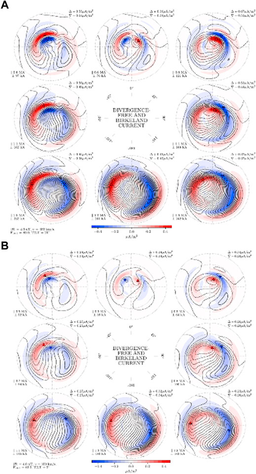
FIGURE 2. Field-aligned current (red and blue color) and the ionospheric Hall currents (black contours), in the Northern Hemisphere in summer (A) and winter (B) seasons (Laundal et al., 2018). The peak upward and downward current densities are listed in the top right corners. Total upward current, labeled by ∥, is given in the lower left corners in units of megaampere. The ionospheric currents are labeled by ┴ in units of kiloampere.

The main peculiarity of current patterns presented in Figure 2A (summer season) is availability of the R1 FAC system with field-aligned currents (∼0.40 μA/m²–0.45 μA/m²) constantly flowing into ionosphere on the morning poleward boundary of auroral oval and flowing out of ionosphere in the evening boundary, irrespective of season and IMF polarity. Additional B_Y currents appear in the day-time cusp region under influence of the azimuthal IMF B_Y component, the current sense being determined by the IMF B_Y polarity. As a result, the R1 field-aligned currents are combined with the B_Y currents in the pastnoon or prenoon sectors depending on B_Y polarity. Under conditions of the northward IMF component the NBZ FAC system is formed poleward of cusp with currents sense opposite to the R1 FAC polarity (∼0.40 μA/m²).

Situation in the winter season (Figure 2B) is quite different: NBZ currents are not observed at all, influence of B_Y FAC system falls to minimum, the R1 FAC intensity falls down to 0.25 μA/m²–0.30 μA/m² under conditions of southward IMF and to 0.05 μA/m²–0.1 μA/m² under conditions of northward IMF. Appearance of specific NBZ or B_Y FAC systems, typical of only summer season, results in essential deformation of DP0/DP2 current system in the summer polar cap. Thus, results (Laundal et al., 2018) demonstrate, in agreement with conclusions (Kuznetsov and Troshichev, 1977; Troshichev and Tsyganenko, 1979) that magnetic activity in polar caps is generated by independent FAC systems, which are different in their structure, disposition and intensity.

3 Idea of PC index

Basing on the above shown results it was suggested (Troshichev, 1982; Troshichev, 1984) that the polar cap magnetic activity, generated by the field-aligned currents responding to IMF variations, can serve as an indicator of the geoeffective solar wind influence on the magnetosphere. The first analysis of the relationships between the solar wind parameters and the polar cap magnetic activity has been fulfilled by Troshichev and Andrezen (1985) using the vector of magnetic disturbances δF observed at the Vostok station (see Section 4.1). Results of this analysis showed that value of δF actually correlates with solar wind parameters and “coupling functions”, as follows:

B_z vertical IMF component R = 0.707

Ei = V_SWB_z (“interplanetary electric field”) R = 0.705

E_T = V_SWB_T (“tangential electric field”) R = 0.665

ɛ = V_SW(B_Y² + B_Z²) sin² (θ/2) (Akasofu, 1979) R = 0.426

E_KL = V_SWB_Tsin² (θ/2) (Kan and Lee, 1979) R = 0.822

As a consequence, the electric field E_KL, defined by formula (Kan and Lee, 1979), was chosen for further analysis

the values E_KL and δF being connected by linear function

where V_SW is the solar wind velocity, B_T is the IMF tangential component B_T=(B_Y²+B_Z²)^1/2, B_Z and B_Y are vertical and azimuthal IMF components, α and β are scale parameters determining linear connection between δF and E_KL, and θ is angle between the IMF B_T component and geomagnetic dipole. It should be noted that practically the same correlation (R = 0.824) is provided by “coupling function” V_SWB_Tsin³ (θ/2), suggested by Reiff and Luchmann (1986). Analogous results have been obtained later when the cross polar cap voltage was estimated by data on the electric field measurements on board EXOS-D spacecraft (Troshichev et al., 1996).

The electric field E_KL was put forward by Kan and Lee (1979) as a “merging electric field” (Em), which is transmitted from solar wind to magnetosphere along the interconnected (merged) interplanetary and geomagnetic field lines. However, it should bear in mind that E_KL field (as well as “interplanetary electric field” Ei = vBz) is not real field born by solar wind, unlike to interplanetary magnetic field (IMF). The “interplanetary” and “merging” electric fields are manifested only in the Earth’s coordinate system, which is stationary in relation to the moved solar wind. In contrast to “interplanetary electric field” Ei, which shows only influence of the southward (BZS) IMF, the “estimated” E_KL field represents the optimal combination of solar wind parameters providing the maximal input of solar wind energy into the magnetosphere. Just this “estimated” E_KL field, inaccessible for immediate measurements, determines magnetospheric convection and generation of real field-aligned R1 currents, accessible for evaluations.

The above presented results have obviously demonstrated that the polar cap magnetic activity (described by the equivalent current system DP2) is linearly related to “estimated E_KL field” and its variations. It meant that efficiency of the solar wind impact on the magnetosphere may be tracked by the ground based magnetic observations, if the relationship between the polar cap magnetic activity and E_KL field is correctly determined for all ranges of solar wind parameters (solar activity), irrespective of state of polar ionosphere (seasonal and daily variations of ionospheric conductitvity) and location of station (disposition of point of observation in the Northern or Southern hemisphere). As a result, the index of polar cap magnetic activity (PC index) was proposed as a measure of the interplanetary electric field coupling with the magnetosphere (Troshichev and Andrezen, 1985).

The idea was appreciated by colleagues from Danish Meteorological Institute (DMI, Copenhagen), responsible for magnetic observations at the northern Thule station. Fruitful collaboration between AARI and DMI started in 1985 and the 15-min PC index was put forward (Troshichev et al., 1988). Data from two near-pole magnetic observatories were used for calculation of the PC index, labeled correspondingly as PCN and PCS indices: station Qaanaaq (known as Thule) in Greenland (corrected geomagnetic latitude 85.4°C, magnetic local noon ∼14UT) and station Vostok in Antarctica (corrected geomagnetic latitude -83.4°C, magnetic local noon 13UT).

4 The PC index derivation method

4.1 Main problems

Even if the DP2 current intensity is not varied, the value of magnetic disturbance, fixed at near-pole station, constantly changes because the station rotating around the geographic pole moves relative to the Sun-oriented ionospheric current system. It means that value of disturbance observed at station will be determined by disposition of station in regard to current system, i.e., by geographic coordinates of the point and UT time. This situation is illustrated schematically in Figure 3, which demonstrates disposition of the northern polar cap and station Thule in the invariant geomagnetic coordinate system (thin black lines) at noon and midnight hours in summer (upper panel) and winter (lower panel) seasons, the geographic coordinate system being shown by thin green lines.

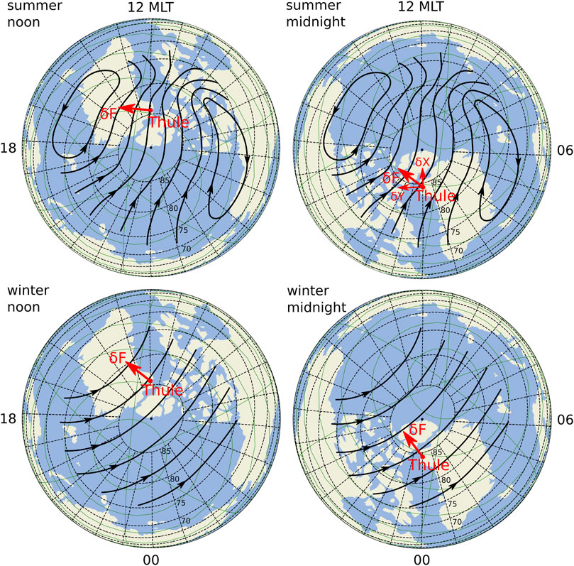
FIGURE 3. Equivalent current systems DP2 (DP0) of magnetic disturbances observed in the northern polar cap at noon and midnight hours in summer (upper panel) and winter (lower panel) seasons.

The sun-oriented equivalent DP2 current system is shown in Figure 3 by thick black lines. Red arrows present the corresponding magnetic disturbance vectors δF (with δX and δY components in upper right figure). In the summer near-pole region these currents are oriented along the Sun–Earth line, in the winter near-pole area the equivalent currents can diverge more 45°C from this direction (Troshichev et al., 1979b). The matter is that magnetic disturbances in the sunlit high-conductivity summer hemisphere are generated by the ionospheric Hall currents, since magnetic effect of the ionospheric Pedersen currents is compensated by magnetic effect of the field-aligned currents, in full agreement with theorem of Fukushima (1969). Consequently, the equivalent DP2 currents are identical to the actual Hall currents flowing in the summer ionosphere. To the contrary, the intensity of ionospheric Hall and Pedersen currents in the dark winter polar cap is marginal, and the polar cap magnetic activity is produced mainly at the account of the R1 FAC distant effect. It means that the winter DP2 system presents the equivalent current system describing mainly the distant effect of the field-aligned currents on the ground surface. Because of this, the equivalent winter DP2 currents are deflected towards dawn through angles 20°C–60°C relative to summer DP2 currents (Maezawa, 1976; Troshichev et al., 1979b).

To take into account the regular variation of magnetic activity, caused by daily rotating the station around the geographic pole, the magnetic disturbance vector δF is calculated according to formula:

where δX·and δY are alterations of the geomagnetic northern X and eastern Y components observed at the station (see Figure 3), λ is the geographic longitude, UT is the universal time, and φ is the UT-dependent angle between the DP2 transpolar currents and the noon-midnight meridian (which is equivalent to angle between the ionospheric electric field and dawn-dusk meridian); signs (+) and (-), valid correspondingly for Vostok and Thule station, are taken to make allowance for opposite polarity of geomagnetic field in the northern and southern hemispheres. Only the horizontal components X and Y are taken into account since the ionospheric currents, flowing above the station, cause horizontal magnetic disturbances underneath the current, likewise the vertical field-aligned currents, flowing in and flowing out of the ionosphere, produce horizontal magnetic deviation on the ground surface. The meaning of expressions (3) and (4) is very simple: they are assigned to arrange the magnetic disturbance vector δF in alignment with DP-2 currents while daily rotating the station under this current system. Since angle φ is subjected to strong daily and seasonal variations, the values of φ should be available for each moment of every day.

Expression (2) implies that the disturbance value F is determined by the E_KL field value, the relationship between values δF and E_KL being strongly dependent on seasonal transformation of the equivalent DP2 currents and disposition of station in regard to the current system. If the scale parameters, i.e., angle φ and the calibration coefficients α and β determining linear connection between δF and E_KL, are statistically justified for any moment of day during the year, they can be taken to calculate the PC index (designed to estimate the E_KL field value) for any actual moment of time with use of δFactual value fixed in this actual time

Thus, the PC index can be calculated at any actual moment UT on conditions that (a) the δX and δY values in expression (3) represent effect of the solar wind influence on magnetosphere, and (b) the scale parameters α, β and φ, determining the relationship between values of E_KL and δF, are statistically justified and always available. The first problem reduces to determining the quiet daily curves (QDC)x and (QDC)y, which serve as level of reference to account off the disturbance values δX and δY related to the solar wind effect. The second problem is correct evaluation of coefficients α (slope) and β (intersection) in expression (2) and angle φ in expression (4) determining the statistically justified relationship between E_KL field and magnetic disturbance value δF for any UT time of every day of year. A line of attack on these problems was put forward in (Troshichev et al., 2006) as “the unified PC derivation metod”, which includes the “QDC running calculation” procedure and determination of statistically justified scale parameters α, β and φ.

4.2 The “QDC running calculation” procedure

The polar cap magnetic observatory constantly registers the geomagnetic field changes, which are separated into two types: regular variations the “quiet” geomagnetic field and accidental magnetic disturbances (magnetic activity) of various origin. The regular daily and seasonal geomagnetic variations are caused by regular change of solar UV irradiation above the observatory in course of daily rotation of station around the geographic pole and seasonal changes in the polar caps illumination in course of the Earth’s rotation around the Sun. The higher UV irradiation is, the larger is conductivity of the polar ionospheric and intensity of electric currents flowing in the ionosphere, and correspondingly, the larger is geomagnetic variations on the ground level. As a result, the QDC magnitude occurred to be maximal at noon during the summer season and to be minimal at midnight during the winter season. Besides, the geomagnetic field demonstrates the regular long-term (∼27 days) variation related to effect of the IMF sector structure (SS effect). In addition, the polar cap ionosphere conductivity is affected also by irregular and powerful solar UV irradiance, related to solar flares in periods of high solar activity, and by the solar proton injections in periods of solar proton events (SPE).

To estimate correctly the polar cap magnetic activity produced by the solar wind impact on magnetosphere it is necessary to separate this activity from the geomagnetic alterations related to solar UV irradiation. The question is easily resolved for regular variation of quiet geomagnetic field: this variation (QDC) is taken as a level of reference to count off the magnetic activity. The SS effect, related to regular changes of the radial IMF component, has not essential action on magnetic activity and may be also included in QDC owing its long duration (∼27 days). The problem is separation of irregular effects of the solar UV irradiance rises, related to solar flares and effects of solar proton events (SPE), which exert a strong influence on the polar cap ionospheric conductivity. If these irregular effects are identified, they can be distinguished and incorporated in QDC which is used as level of reference to evaluate the magnetic activity produced by the solar wind.

The problem with the irregular solar UV irradiation rises related to solar flares was solved taking into account the crucial distinction between typical duration of the E_KL field changes produced by the geoeffective solar wind (from minutes to hours) and the duration of effects produced by the irregular UV irradiation rises (several days). Consideration of the solar flares effect as the long-term factor in comparison with the short-term solar wind (E_KL) factors made it possible to distinguish this irregular effect and to include it in the level of reference (QDC) (Troshichev et al., 2006). The problem with SPE effect, with duration from 1 day to some days, remains unresolved.

Figures 4A–D illustrates, on the example of geomagnetic X component for the Vostok station, the operations forming the “QDC running calculation” procedure. The upper panel shows the real run of geomagnetic X component (B_x) during year 2000 (the summer months at Vostok station are November/December/January/February and the winter months are May/June/July/August). Figure 4B demonstrates separation of the SS effect in X component (ss_x). Taking into account the strong periodicity (∼27 days) of the IMF sector structure, the SS effect is separated on the basis of data for 3 previous months, using a 7-days smoothing window. One can see that SS effect at Vostok station is noticeable in period from October to March and negligible in period from April to September. Figure 4C shows the difference B_x-ss_x, the essential changes being seen in value of geomagnetic alterations in summer months after subtraction of the SS effect. The same procedure is performed for geomagnetic Y component registered at station.

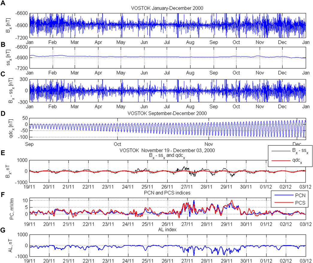
FIGURE 4. (A–D) Four stages of the “running QDC calculation” procedure (on the example of geomagnetic X component); (E) Run of geomagnetic quantity δX = B_x-ss_x (black line) and the appropriate quiet daily variation QDC_x (red line) at Vostok station in November 2000; corresponding alternations of the appropriate PCN and PCS indices (F) and AL index (G) for period from 19 November 2000 to 02 December 2000.

Just geomagnetic variation shown in Figure 4C was used for separation of 5 quiet days (or quietest segments) within the interval of 30 previous days to deduce the QDC for current day. The QDC is automatically recalculated for each particular day, the results being extrapolated for the subsequent day with aim of the on-line estimation of QDC and derivation of the quicklook PC index in this day (preliminary PC index is obtained after recalculation of QDC for elapsed day). Figure 4D shows the QDC shape for X component for each particular day in period from September 2000 to January 2001 (the different scale of quantities on panels (A)–(D) should be taken into account). It is seen that the QDC amplitude systematically increases during this period (from minimum in September to maximum in December/January), but some less-scale variations travel in waves against the background of this regular seasonal variation, since the QDC time evolution includes the irregular increases in UV irradiation related to solar flares. It implies that the QDC behavior is changed from year to year, the QDC amplitude being maximal on years of solar activity maximum and being minimal on years of solar activity minimum.

The “QDC running calculation” procedure was used in AARI from the outset. In Danish Meteorological Institute (DMI), which was responsible for magnetic observations at Thule stations up to 2011, the distinct method, described by Vennerstrøm (1991), was used for the PCN index production. The “quiet level” in this method is determined by interpolation between the absolute values of geomagnetic field, established at nighttime hours of quiet winter days in the two consecutive years. Unfortunately, the “unified PC derivation method” (Troshichev et al., 2006) has not been adopted in DMI since the competitive method, named as a solar rotation weighted (SRW) method, was suggested by Stauning (2011).

The SRW method makes allowance for “the steady or recurrent variations in the magnetic field components during quiet conditions with time-of-day, day-of-year, and solar activity level”. According to concept of Stauning (2011), the solar influence on the geomagnetic activity is regularly repeated due to solar rotation, resulting in steady or recurrent variations (with period ∼27 days) in the IMF sector structure, in the solar wind velocity and in the 10.7 cm radio flux (F.10.7). The SRW method includes the weight factors, which promote the samples separated by one solar rotation “having the same face on the Sun turned toward the Earth” and enhance the importance of nearby samples, but minimises “the samples measured with the opposite face of the Sun turned toward the Earth”. It means that the SRW-method emphasizes the regular 27-days periodicity (“sector structure”) and levels off the irregular effects without this periodicity. As a result, the effects of the irregular solar UV rises related to solar flares can be automatically attributed to the PC index value, which is counted off from QDC, determined by SRW method. It should be noted that the “unified method” (Troshichev et al., 2006) has been recommended by IAGA Division V-DAT, as the best, for the IAGA endorsement and has been approved by IAGA in 2013.

Analysis of the QDC amplitude changes conditioned by the solar UV irregular variations has been fulfilled in (Troshichev et al., 2021) basing on yearly values of QDC magnitude and solar UV irradiance for period of 23/24 solar activity cycles. It is well known that the ionosphere conductivity is ensured by the solar X and UV irradiation with wavelength 100 nm–200 nm, which is absorbed in the Earth’s upper atmosphere and ionosphere (50 km–500 km), the radiation being varied in range of 20% (0.1 W/m² ± 0.02 W/m²) in connection with solar flares. The data on UV (100 nm–200 nm) irradiance (https://lasp.colorado.edu/lisird/data/lasp_gsfc_composite_ssi/) were used to examine the relation between the QDC magnitude and the solar irradiance level. The yearly-averaged amplitudes of QDC for X and Y components at stations Thule and Vostok were taken and their summary values (QDCtotal_X and QDCtotal_Y) were counted for each year. It turned out that the yearly values QDCtotal_X and QDCtotal_Y demonstrate the same regularity in alterations from year to year.

Figure 5 shows run of the yearly values of QDCtotal_X, QDCtotal_Y (a) and UV irradiation 150 nm–200 nm (b) in 1998–2018. One can see the well correspondence between the alterations of yearly values of QDCtotal magnitude and appropriate UV irradiance during this period. Figure 5C shows, as example, the correlation between values of the QDC magnitude and UV irradiance 160 nm, which is as high as R = 0.943. This perfect correspondence between the alterations of UV and QDC quantities demonstrates strong dependence of the QDC magnitude on solar activity (solar flares) and verifies correctness of the “running QDC calculation” procedure (Troshichev et al., 2006) used for derivation of the PC index.

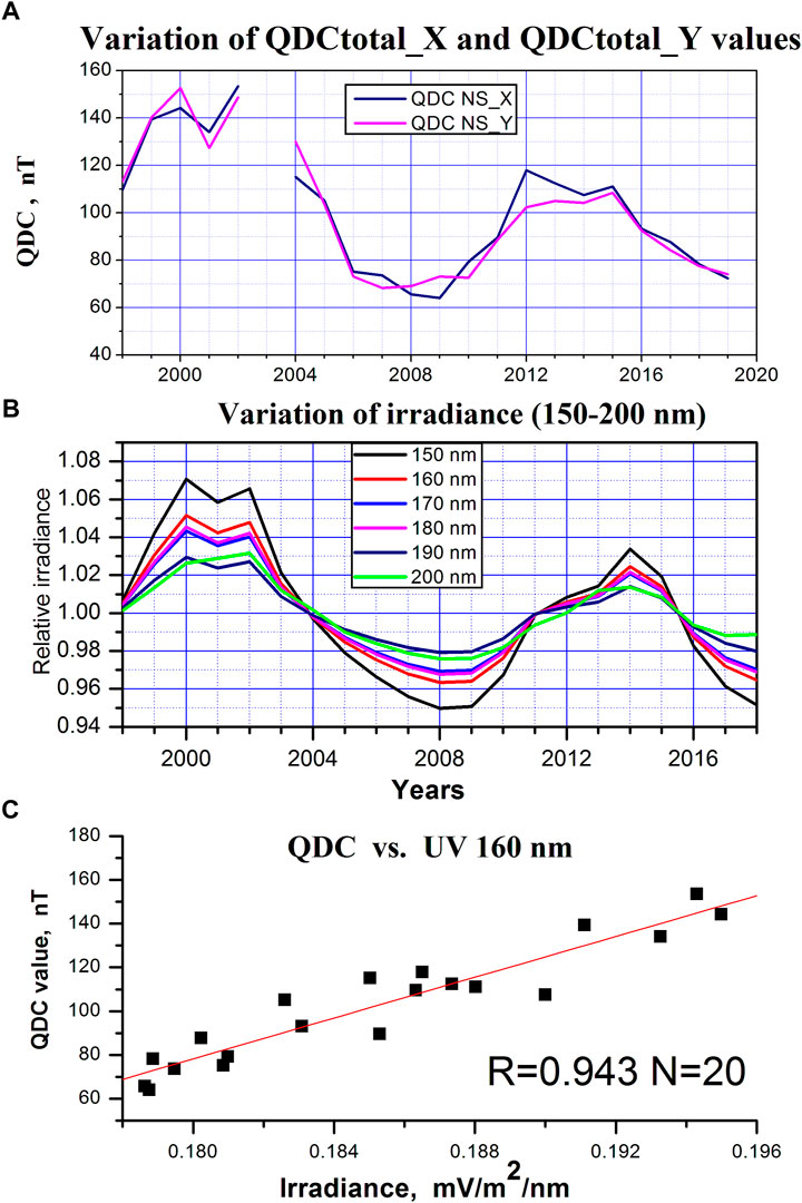
FIGURE 5. Run of yearly values of QDCtotal_X, QDCtotal_X (A) and solar UV (150–200 nm) irradiation (B) during 1998–2018 and correlation between the corresponding yearly values of UV(160 nm) and QDCtotal (C) (Troshichev et al., 2021).

4.3 Determination of statistically justified scale parameters α, β and φ

To determine calibration parameters, the E_KL values were calculated according Eq. 1 by data on solar wind parameters presented at OMNI site (http://omniweb.gsfc.nasa.gov). The appropriate δF values, representing the DP2 disturbances at near-pole stations Thule and Vostok, were evaluated with use of the “running QDC” as a proper level of reference. The coefficients α and β, determined linear connection between δF and E_KL, were calculated for all values of angle φ in the range of ± 90°C from the suggested dawn-dusk orientation of DP2 vector. The “true” angle φ was chosen as angle value providing the best correlation between values δF and E_KL, and the quantities α, β corresponding to this “true” angle φ, were regarded as optimal, statistically justified parameters.

At first, the statistically justified parameters α, β and φ were calculated for epochs of solar maximum (1998–2001) with use of the GSE (Geocentric Solar Ecliptic) representation (Troshichev et al., 2006). In 2009 the parameters were recalculated with use of the GSM (Geocentric Solar Magnetosphere). Then the justified parameters were determined (with use of the GSM presentation) for epoch solar minimum (1997, 2007–2009) and for a complete cycle of solar activity (1995–2005) (Troshichev et al., 2006). Figure 6 shows these 3 series of parameters determined for Vostok station in these epochs (left, middle and right columns) as function of UT time (axis of abscises) and month (axis of ordinates). One can see that patterns for angles φ (denoted here as Φ) and coefficients α and β, derived at a quite different level of solar activity, are in good conformity by character and amplitude in course of UT and season changes (the difference in scales for three columns should be taken into account), testifying that the relationship between E_KL and δF remains basically the same irrespective of solar activity cycle. As a result, α, β and φ parameters obtained with use of the GSM representation for the full cycle of solar activity 1995–2005 (right column in Figure 6) were applied in all subsequent analyses.

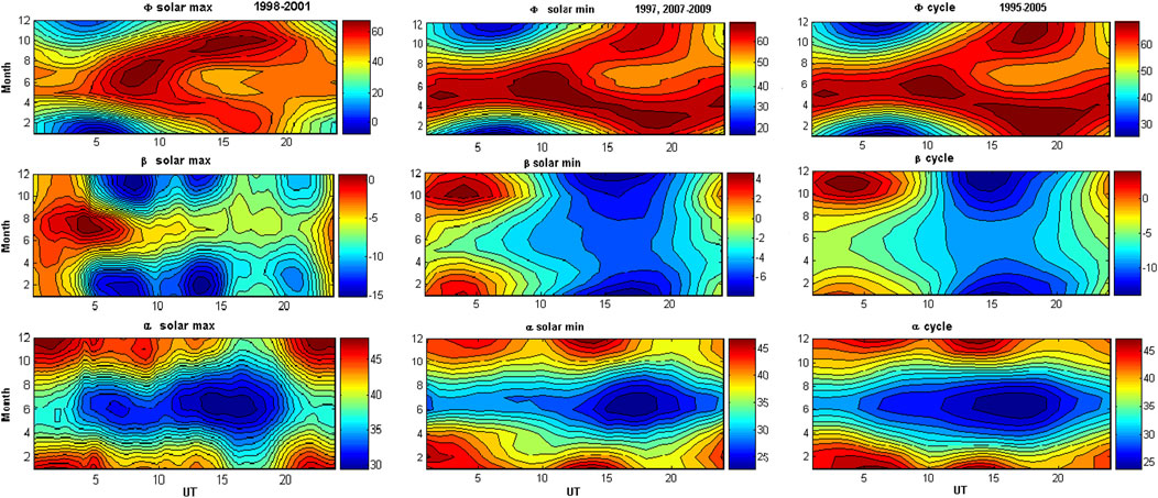
FIGURE 6. Parameters Φ (1st panel), β (2nd panel) and α (3rd panel), derived for the Vostok station for epochs of solar maximum (left column), solar minimum (middle column), and for the full cycle of solar activity 1995–2005 (right column), the axis of abscises being for UT and axis of ordinates being for month (Troshichev et al., 2011a).

The main peculiarity in behavior of calibration parameters is a seasonal dependence of parameters α (slope), β (intersection) and Φ (angle between the DP2 transpolar currents and noon-midnight meridian). Parameter α reaches the maximal value during summer months at Vostok station (January/February and November/December) and reduces in half during the winter months (May/June/July/August) suggesting the strong dependence of δF value on ionospheric conductivity. Transpolar currents are close (Φ ∼ 20°C) to noon-midnight meridian during 0–12 UT in summer and deviate up to 60°C from the meridian in winter, the seasonal distinction being conditioned by the different nature of the magnetic disturbances in the summer and winter polar caps. Availability of statistically justified parameters α, β and φ made it possible to calibrate the δF quantities by E_KL values. As a result, the stations Thule and Vostok, located in different points of the northern and southern polar caps and referred to different α, β and φ parameters, yield the similar PCN and PCS indices, consistent with value of E_KL field affecting the magnetosphere.

4.4 Derivation of PC index

Figure 4E shows, in a large scale, the run of values δX = Bx-ss_x (where ss_x is the SS effect for X component) and QDC_x (which were presented in Figures 4C,D) for period from November 19 to 02 December 2000 at Vostok station. The deviations of values δX = B_x-ss_x and δY = B_y-ss_y from the appropriate values of QDC_x and QDCy at the Thule and Vostok stations were taken for calculation of the corresponding PCN and PCS indices with use of the statistically justified parameters α, β and φ available for any current moment of any day of year. Figure 4F demonstrates the PCN (blue) and PCS (red) indices derived by “unified method” for the indicated period. Figure 4G shows, for comparison, the run of magnetic disturbances in the auroral zone (AL index). One can see a good conformity between alterations of the AL and PCN, PCS indices, in spite of fact that these indices, derived from absolutely independent series of magnetic data, characterize magnetic activity in quite different regions of the magnetosphere. It implies that PC index really estimates input of solar wind energy into the magnetosphere (Troshichev and Janzhura, 2012; Troshichev, 2017).

4.5 Problem of negative PC index

In spite of the fact that the R1 FAC system acts at all times, irrespective of the IMF B_Z sign, the PC index in summer polar cap (PCsummer) often demonstrates the negative meanings (see Figure 4F). The negative PC indices are related to NBZ FAC system acting in the limited sunlit near-pole region (Armstrong and Zmuda, 1970; Zmuda and Armstrong, 1974; Iijima and Potemra, 1976b; Iijima et al., 1978). Corresponding DP3 current system is generated in borders of this area on the background of DP2 current system. As a result, the forth-vortices current system is formed in the summer polar cap without essential changes in structure of DP2 currents at latitudes below 75°C (see Figure 2A, upper panel). Under these conditions, the PCsummer index is incapable to elucidate situation in the entire polar cap. At the same time, the R1 FAC structure in the winter hemisphere remains invariable and intensity of the DP2 disturbances is taken into account by the corresponding PCwinter index. It means that the solar wind impact on the magnetosphere under conditions of the northward IMF should be estimated by the PCwinter index, the negative PCsummer indices can be used only for identification of current situation in the summer polar cap (for example, as indicator of magnetic quiescence).

5 Realization of idea. Preliminary and definitive PC indices

As a result of collaboration between Danish Meteorological Institute (DMI) and Arctic and Antarctic Research Institute (AARI), the 15-min PC index was put forward (Troshichev et al., 1988). The results of subsequent studies (Vennerstrøm, et al., 1991; Troshichev et al., 1996; Vassiliadis et al., 1996; Takalo and Timonen, 1998; Liou et al., 2003) showed that the PC index growth is followed by magnetic disturbances in the auroral zone, the substorm intensity (AL index) and auroral power being well correlated with PC index. Transition to 1-min PC index, carried out independently in AARI and DMI, was completed by 1999, the principles of the PC derivation being unchanged. However, inconsistency between the PCN and PCS values produced, correspondingly, in DMI and AARI was revealed as a regular phenomenon (Lukianova et al., 2002). The main reason for this inconsistency was the difference in reference levels (QDC), which were used in DMI and AARI to account off the magnetic disturbance values δF (see Section 4.2). It became evident that the unified method for PCN and PCS derivation is required to eliminate any influence of the calculation technique on results of the analysis (it is one of the obligatory IAGA requirements to approve the index). To resolve the problem, the unified method of PC index derivation, basing on procedure elaborated in AARI, was put forward (Troshichev et al., 2006), but this method has not been adopted in DMI.

In 2009 the IAGA Division V-DAT appointed a special Task Force for examination of the PC index long-standing issue. The Task Force team fulfilled the comprehensive analysis of three competitive methods offered for examination: (1) the “unified method” (Troshichev et al., 2006), (2) the official DMI method (Vennerstrøm, 1991) and (3) the SRW method (Stauning, 2011). As a result, in 2010 the “unified method” (Troshichev et al., 2006) has been recommended by IAGA Division V-DAT, as the best, for the IAGA endorsement (see McCreadie and Menvielle, 2010). In the same year the Space Institute of the Danish Technical University (DTU-Space) became responsible for magnetic observations at Thule station, and AARI and DTU get agreement on all details of the PC derivation procedure based on the “unified method” (Troshichev et al., 2006). In 2013 the new PC index, produced by the unified method, was approved by IAGA (IAGA resolution, 2013). In 2014 the PCN and PCS indices for all previous years were recalculated with application of “the unified method” and use of calibration parameters α, β and φ obtained for the full cycle of solar activity (1995–2005).

According to the IAGA rules, all indices obtained by data of current magnetic observations are considered as “provisional” ones. They should be checked afterwards making allowance for all possible faults of observational, technical and computer-assisted origin, to produce the “definitive” indices, which should be valid for ever. This work was fulfilled in AARI and DTU Space in 2021 with use of the modernized code (Nielsen and Willer, 2019). Comparison of the provisional and definitive PCN and PCS indices for 24 years (1997–2020) has demonstrated perfect agreement between the appropriate definitive PCN and PCS indices and only incidental differences between the series of provisional and definitive PC indices. Consequently, the definitive PCN and PCS indices were finally approved by IAGA and the PC index was recommended for use by the international scientific community (IAGA resolution, 2021). The definitive series of the PCS and PCN indices for 1997–2020 are presented at web-sites http://pcindex.org; http://isgi.unistra.fr; ftp://ftp.space.dtu.dk/WDC/indices/pcn/.

6 Relation of PC index to the solar wind E_KL field

6.1 Relationship between the 1-min values of E_KL field and PC index

The relationship between the 1-min E_KL and PC values during active periods was studied by Troshichev and Sormakov (2015) on the basis of isolated and expanded substorms for 1998–2001 listed in (Troshichev et al., 2014). Values of E_KL field were calculated using the data on solar wind parameters reduced to magnetopause (OMNI/Web interface http://omniweb.gsfc.nasa.gov). To level off an occassional magnetic activity asymmetry in the opposite polar caps, the PC index was taken as an average value of the PCN and PCS indices. The total number of examined events with data available for both stations turned out to be N = 163 for the isolated substorms, N = 983 for the expanded substorms, and N = 261 for the coordinated events for the period of 1998–2001.

Two approaches were used while performing the analysis. In the first approach the correlation between the E_KL and PC quantities was calculated in the 1-h interval preceding the sudden onset (SO) of each isolated or expanded substorm, the SO moment being used as a key date T₀. In the second approach the events with the conforming PC and E_KL deviations on the 2-h interval preceding SO were separated as coordinated events, the E_KL field raise commencement was taken as a key date (T₀), and the correlation between the E_KL and PC quantities over the time period T₀ ± 30 min was examined. In both cases the correlation between E_KL and PC was described by linear function, the coordinated E_KL and PC increases being followed by the substorm onsets.

Figure 7 shows degree of correlation between the E_KL field and PC index for all three types of substorms (upper panel) and distribution of delay times in response of PC index to changes in E_KL field (lower panel). To reveal the optimal time of the PC response to E_KL changes, the consideration of delay time was restricted to the most representative events demonstrating the correlation R > 0.75 between the PC and E_KL quantities smoothed with use of the 15-min running window. As Figure 7 demonstrates, the delay times are extended in the range from 0 min to 40 min with the pronounced peak at ΔT = 10 min–18 min for isolated substorms, ΔT = 10 min–20 min for extended substorms and ΔT = 13 min–18 min for coordinated events. The presented results testify that the PC index growth preceding the substorm onset is strongly related to the appropriate raise of E_KL field.

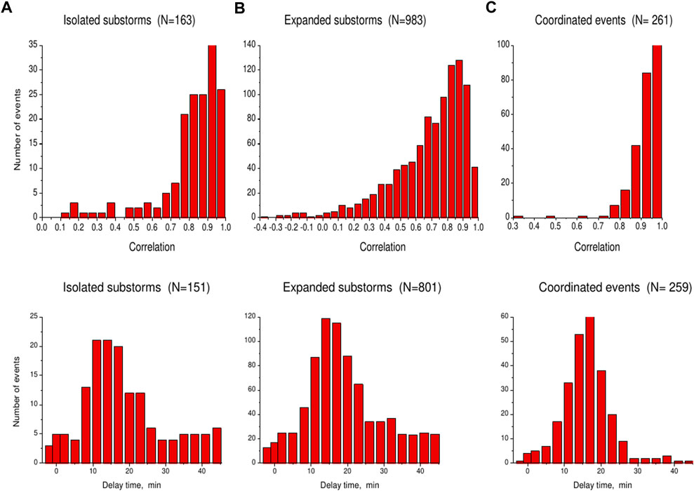
FIGURE 7. Histograms demonstrating values of correlation between the E_KL field and PC index (upper panel) and delay time in response of PC index to E_KL alterations (lower panel) for events with isolated (A), expanded (B) and coordinated (C) substorms (Troshichev and Sormakov, 2015).

The comparative analysis of the substorm behavior in relation to the E_KL field and PC index was also fulfilled in (Kullen et al., 2010; Despirak et al., 2016). 874 substorms with and without growth-phase pseudobreakups were studied by Kullen et al. (2010). It was shown that the E_KL field rise can be observed about 1 h–2 h before the substorm onset. However, in this case the E_KL rise is slow and gradual (growth rate <0.04 mV/m/min) and does not exceed the critical level ∼1.5 mV/m, whereas the substorm demonstrates very low intensity (AE ∼ 200 nT). The substorms appear as isolated events after some hours of low geomagnetic activity. According to classification given in (Troshichev et al., 2014), these events refer to category of isolated substorms with growth phase lasted long time without sharp increases of the PC index.

Over 1,700 substorms, observed during two solar cycle maxima (1999–2000 and 2012–2013) were studied by Despirak et al. (2016). The substorms were divided into 3 types according to auroral oval dynamic: substorms which were observed only at auroral latitudes (“usual” substorms), substorms which propagate from auroral latitudes (< 70°C) to polar geomagnetic latitudes (> 70°C) (“expanded” substorms) and substorms which are observed only at latitudes above ∼70°C in the absence of simultaneous disturbances below 70°C (“polar” substorms). It was found that different PC values were typical of these types of substorms: the highest PC index values were observed before the “expanded” substorms, the lowest PC values were observed before the “polar” substorms.

6.2 Factors, controlling delay in response of PC index to the E_KL field alterations

To determine factors controlling the delay time in the PC response to E_KL field changes, Troshichev and Sormakov (2015) examined relation of the delay time value ΔΤ to such solar wind parameters, as the IMF vertical (B_Z), azimuthal (B_Y), and horizontal (B_T) components, the solar wind speed (V_X) and dynamic pressure (Pdyn), the parameters being averaged for the 1 h term preceding the SO moment (T₀). Contrary to expectations, the role of any separate solar wind parameter in the substorm development occurred to be insignificant. As this takes place, correlation between PC index and E_KL field was evident. Thereafter the “coordinated events”, with conforming behavior of PC index and E_KL field on the 2-h interval preceding SO, were examined.

Coordinated events were divided into different groups according to value of delay time ΔT. Figure 8 shows behavior of the smoothed values of V_X, B_Z, E_KL and PC in course of coordinated events for the statistically justified groups with ΔT = 10 min–12 min (N = 33), ΔT = 13 min–15 min (N = 53), ΔT = 16 min–18 min (N = 60), and ΔT = 19 min–21 min (N = 38), the font size shown on the left side is the same for all intervals of ΔT. Thin red lines represent the time evolution of V_X, B_Z, E_KL and PC in course of individual events. Solid black lines show the behavior of the mean V_X, B_Z, E_KL and PC quantities for each ΔT group. Vertical lines mark the delay time interval boundaries T₀ and T₀ + ΔT, the latter corresponds to the moment when the PC index starts to increase.

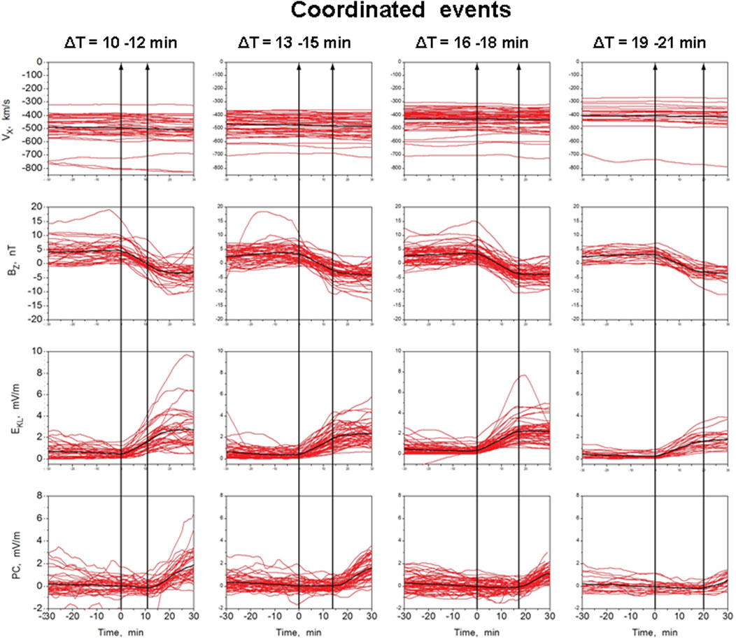
FIGURE 8. Time evolution of the 15-min smoothed values V_X, B_Z, E_KL and PC observed in case of coordinated substorm events with delay times ΔT = 10–12, 13–15, 16–18, and 19–21 min (Troshichev and Sormakov, 2015).

Figure 8 (upper panel) shows that the delay time tends to increase while the mean value of solar wind │V_X│ decreases. Nevertheless, the solar wind speeds V_X, as large as −800 km/s and as small as −300 km/s, are common for any ΔΤ group. Besides, the time evolution of V_X is not responsive to moment T₀. The IMF vertical B_Z component (2nd panel) starts to turn down (southward) just at moment T₀, the regularity being evident for individual events, as well as for mean B_Z in each ΔΤ group: the higher the B_Z alteration magnitude (ΔB_Z) is, the shorter the delay time ΔT is. However, the larger ΔB_Z values are built up at the expense of positive (northward) B_Z preceding the moment T₀, whereas the base level of negative (southward) B_Z after the T₀ was ∼ −3.5 nT for all ΔΤ groups. At the same time, correlation between ΔΤ and E_KL field (3rd panel) turns out to be quite explicit: the higher the E_KL rise (ΔE_KL) during the ΔT interval, the shorter is the delay time ΔT in response of PC to the E_KL rise. The actual delay time is determined by the E_KL field growth rate, not by such solar wind parameters, as IMF B_Z component or solar wind speed V_X (averaged for 1-h interval preceding the substorm sudden onset). The shortest delay times (ΔΤ < 10 min) were related to significant strengthening of southward IMF and a rather low speed of solar wind (V_X ∼ 350 km/s–450 km/s).

6.3 Inconsistency between the PC index and E_KL field in particular cases

General link between the E_KL field and PCN, PCS indices is determined by parameters α, β and φ, characterizing relationships between the disturbances values δF, observed at stations Thule and Vostok, and values of E_KL, estimated by data presented at site (http://omniweb.gsfc.nasa.gov). These parameters were derived for period from 1995 to 2005 (Troshichev et al., 2011a) and are regarded as statistically justified. Nevertheless, in particular events the relationship between PC index and E_KL field can strongly deviate from statistical regularity. Troshichev and Sormakov (2019b) have analyzed relationship between the E_KL and PC values for 1,302 substorm events and found that well correlation (R>0.5) between E_KL field and PC index was observed in only ∼80% of the examined substorms. Typical examples of consistency and inconsistency between E_KL field and PC index are presented in Figure 9, where the upper panel shows behavior of E_KL field (green) and index PCmean = (PCN + PCS)/2 (violet), the middle panel is for PCN and PCS indices (blue and red lines), the lower panel shows the magnetic disturbance indices AL/AU, the substorm onsets being marked by vertical dotted line.

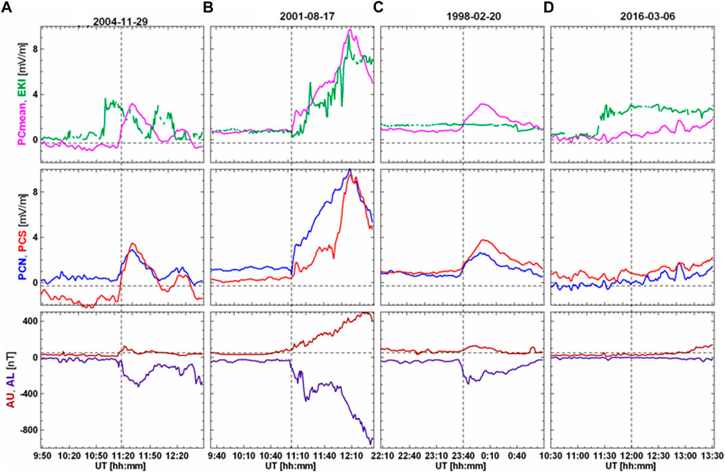
FIGURE 9. Examples of coordinated changes of EKL field and PCmean index (upper panel), PCN and PCS indices (middle panel), AU and AL indices (lower panel) in course of isolated magnetic substorms (Troshichev and Sormakov, 2019b): (A) Disturbance started against the background of quiet magnetic field in connection with the PC growth responding to the EKL field increase; (B) Jump of PC index and the substorm onset was registered ∼10 min ahead of the appropriate EKL field increase on the magnetopause; (C) The EKL field was unchanged and quiet, whereas PC index demonstrated jump above 2 mV/m, which was accompanied by the substorm development; (D) The EKL field demonstrated long increase above 2 mV/m but this increase was not followed by the PC index growth and substorm development.

Figure 9A demonstrates coordinated changes of E_KL, PC and AL values in course of isolated magnetic substorm on 29 November 2004, when the disturbance started against the background of quiet magnetic field in connection with the PC growth responding to the E_KL field increase. Figure 9B demonstrates specific event on 17 August 2001, when jump in PC index was registered ∼10 min ahead of the appropriate E_KL field increase on the magnetopause. Since E_KL field is estimated by data on the solar wind parameters measured by spacecrafts far upstream of the magnetosphere, it is logically suggest that the actual solar wind, fixed by distant monitors, traveled in space with acceleration in this case. As a consequence, the real contact of solar wind with magnetosphere (and jump of PC index) occurred ahead of the “estimated” contact.

Figures 9C,D give examples of events when the magnetic activity (PC and AU/AL indices) was not consistent at all with the E_KL field alterations. In case of events on 20 February 1998 electric field E_KL was unchanged and quiet (E_KL ∼1 mV/m), whereas PCN and PCS indices demonstrated jump above 2 mV/m, which was accompanied by development of substorm with intensity of AL ∼ -400 nT. In case of event on 06 March 2006 the E_KL field demonstrated sharp increase above 2 mV/m for long, but this increase was not followed by the PC index growth and substorm development. As analysis (Troshichev and Sormakov, 2019b) has demonstrated, correlation between the PC and E_KL field was poor or even negative in about 20% of examined events, in spite of the evident consistency in variations of PC and AL indices. It means that IMF, measured by the distant solar wind monitors, did not encounter the Earth’s magnetosphere at all in these cases or impact on the magnetosphere by side-flow.

This conclusion is in full agreement with results (Vokhmyanin et al., 2019), which have demonstrated that the solar wind parameters measured in the Lagrange point and in vicinity of the magnetosphere (data of Geotail spacecraft in front of the magnetosphere bow shock obtained for 10 409 intervals available in both datasets over the period from 1997 to 2016) were distinguished in ∼25% of the examined intervals irrespective of the space weather conditions. It is particularly remarkable that according to Vokhmyanin et al. (2019), both sets of data (the OMNI database and the Geotail measurements) turn out to be in a good agreement in those cases when the PC index correlated well with the E_KL field derived from the OMNI data.

Thus, the correspondence between PC index and E_KL field is often missing details or disappears, in spite of statistical conformity of these two quantities. This circumstance seems to be quite reasonable since the estimation of the E_KL value is based on measurements of the solar wind parameters far upstream of the Earth, usually near the Lagrange point (at distance of ∼1.5 million km). The actual E_KL field coupling with the magnetosphere can be distinct from the “estimated” E_KL field for the following reasons:

1) The IMF has a small correlation distance (within 60 Earth radiuses of the Sun-Earth line) compared to solar wind plasma properties (King and Papitashvili, 2005). The spacecrafts should be positioned within this distance to monitor correctly the solar wind components.

2) The solar wind, measured by distant solar wind monitor, traveled in space with acceleration. As a consequence the real contact of solar wind with magnetosphere (and jump of PC index) occurred ahead of the “estimated” contact time (∼2% of the examined substorm events).

3) The solar wind, whose parameters are fixed by monitors far ahead of the magnetosphere, are not meet the magnetosphere at all, or contact with the magnetosphere by side.

6.4 Relationship between the daily values of E_KL field and PC index

Analysis of general relationship between the PC and E_KL values for 24 years (1997–2020) was fulfilled in (Troshichev et al., 2022) basing on the daily averaged quantities of E_KL field and definitive indices PCN and PCS. Figure 10 shows, as example, variations of the daily quantities of E_KL field and definite PCN, PCS indices in years of increased solar activity (2000 and 2015) and in years of solar minimum (2008 and 2019).

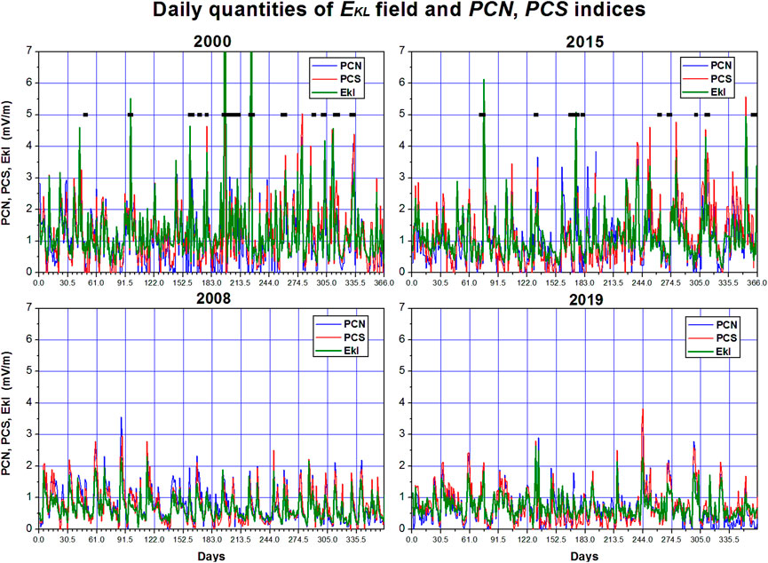
FIGURE 10. Courses of the daily quantities of E_KL field and definitive PCN and PCS indices in years of increased solar activity (2000, 2015) and in years of solar minimum (2008, 2019). Black strips mark days with SPEs (Troshichev et al., 2022).

One can see that the daily E_KL and PCN, PCS quantities in periods with increased solar activity (upper panels) often exceed the value ∼1.5 mV/m, which presents a threshold level for development of magnetic disturbances (Troshichev et al., 2014). In epochs of solar minimum (lower panels) the daily PCN, PCS and E_KL quantities were generally lower this level. The daily PC and E_KL quantities alter (leap or drop) in perfect correspondence: the traces of PCN (blue) and PCS (red) usually do not go beyond the olive trace of E_KL. The relationship between the daily values of E_KL field and PCN, PCS indices is described by the linear function (with coefficient of correlation R) irrespective of the epoch and phase of solar activity.

2000 PCN = 0.039 (± 0.048) + 0.822 (± 0.029) *E_KL (R = 0.833)

PCS = 0.139 (± 0.048) + 0.836 (± 0.028) *E_KL (R = 0.839)

2008 PCN = -0.075 (± 0.027) + 1.336 (± 0.035) *E_KL (R = 0.893)

PCS = -0.108 (± 0.025) + 1.31 (± 0.032) * E_KL (R = 0.905)

2015 PCN = 0.013 (± 0.055) + 0.936 (± 0.04) * E_KL (R = 0.779)

PCS = -0.096 (± 0.048) + 1.116 (± 0.035) * E_KL (R = 0.86)

2019 PCN = -0.215 (± 0.03) + 1.282 (± 0.037) * E_KL (R = 0.876)

PCS = -0.21 (±0.03) + 1.335 (± 0.037) * E_KL (R = 0.886)

As study (Troshichev et al., 2022) showed, decrease of correlation between E_KL field and PC indices below 0.85 was observed in periods of solar maximum, involving intervals of high magnetic activity with daily quantities of PCN, PCS and E_KL exceeding the value ∼4 mV/m. These intervals were related to solar proton events (SPE), when invasion of the high-energy solar protons produces the extreme increase of ionosphere conductivity in both polar caps. Strong correlation (R = 0.88) between the geomagnetic deviations at the polar stations Thule and Resolute Bay and PC and AE indices during major SPE events was demonstrated by Khan et al. (2013). In Figure 10 intervals with SPE in 2000 and 2015 are marked by horizontal black strips (according to catalogs of Logachev Yu et al., 2016; 2022), the solar proton events being absent in 2008 and 2019. If the intervals with SPE events are excluded from examination, the correlation between the daily quantities of E_KL field and PC index is increased up to R = 0.875 in 2000 and up to R = 0.87 in 2015. The SPE related effect is not identified by the “QDC running calculation” procedure as the extreme increase of ionospheric conductivity in view of short duration of the phenomenon (from hours to tens hours). As a result, effect of the ionospheric conductivity increase is attributed to the solar wind influence that led to decrease of correlation between the E_KL field and PCN/PCS indices in these cases.

Results of the analyses (Troshichev et al., 2022) testify that relationship between the solar wind electric field E_KL and the polar cap magnetic PC index (correlation on level R > 0.875 with decrease to R < 0.80 in epochs of solar maximum) was not changed when passing from 23rd to 24th solar cycle, in spite of high difference of these cycles in activity. It means that calibration parameters, determining these relationships, can be regarded as valid irrespective of the solar activity cycle.

6.5 Variations of PC index and solar wind parameters in course of 23/24 solar activity cycles

Keeping in mind the evident link between E_KL field and PCN, PCS indices, the alteration of the yearly values of E_KL and index PCmean = (PCN + PCS)/2 during the 23/24 cycles was examined by Troshichev et al. (2021) in relation to such solar wind parameters, as solar wind velocity Vsw, total IMF field |B|, southward IMF Bz component, solar wind density Nsw, velocity Vsw² and the solar wind dynamic pressure Pdyn = mNswVsw². The yearly values of the solar wind parameters Vsw, Nsw, Pdyn, IMF B|, By, Bz, E_KL were counted from the corresponding hourly (or daily) data presented on website http://omniweb.gsfc.nasa.gov. The “relative” yearly values of these parameters (i.e., the yearly quantities of various indicators, normalized by their averaged value for 22 years) were used to ensure the descriptive comparison of parameters with quite divergent scales of magnitude. It should be remembered in this connection that correlation between the compared quantities remains the same whether absolute or relative values are taken.

Results presented in Figure 11A (Troshichev et al., 2021) show that the yearly values of PCmean are closely related to such solar wind parameters as the solar wind velocity Vsw (R = 0.86) and the IMF intensity |B| (R = 0.84), resulting in high correlation of PCmean with their product, field E_KL (R = 0.92). It is remarkable that yearly PC index correlate with IMF |B| value much better than with the IMF Bz component (R = 0.72), much like E_KL field, which correlation with |B| is as high as R = 0.96 compared to correlation with B_Z (R = 0.81). The magnetospheric disturbance indices, AE and Dst, demonstrate the same regularity: the correlation of AE and Dst with |B| is equal to R = 0.88 and R = 0.86, whereas their correlations with Bz is equal to R = 0.69 and R = 0.74, correspondingly. It implies that dependence of magnetic disturbances on value of total IMF field |B| is stronger than their dependence on the IMF Bz component, in spite of high geoefficiency of the IMF southward (Bs) component.

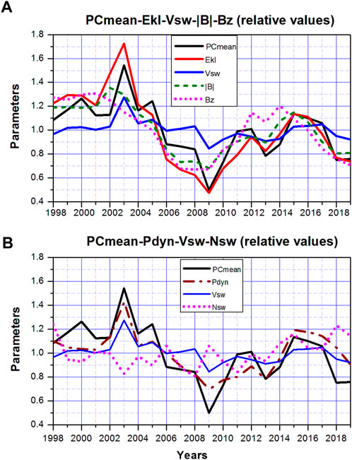
FIGURE 11. Alteration of relative yearly values of E_KL, Vsw, Bz, |B| (A) and Pdyn, Vsw, Nsw (B) along with variation PCmean over a period of 1998–2019 (Troshichev et al., 2021).

The yearly PCmean values well correlate also with yearly Pdyn (R = 0.83) values (Figure 10B), however this linkage is evidently provided by solar wind velocity Vsw (R = 0.86). The other constituent, the solar wind density Nsw, demonstrates negative correlation with PCmean (R = -0.27) as well as with Vsw (R = -0.42) and E_KL (R = -0.08). This regularity is consistent with results presented in Section 7, which show that the PC index correlates with the Pdyn impulses only if these pulses are accompanied by corresponding changes in E_KL field, the inconsistency between the Pdyn and PC alterations becoming evident when the E_KL and Pdyn courses diverge.

6.6 Cross-polar cap voltage and electric field

Interrelation between PC index and cross-polar cap voltage (and diameter) was examined firstly in (Troshichev et al., 1996) with use of data of the particle and electric field measurements on board EXOS-D (Akebono) satellite for period January-June 1990. As results of the analysis showed, both parameters, polar cap diameter and voltage, well correlate with PC index. The same result was obtained (Troshichev et al., 2000) when examining the ionospheric electric field derived from the ion drift measurements made by DMSP satellites over the near-pole region, the PCN and PCS indices being used in the analysis (Figure 12). According to Chun et al. (2002), the cross polar cap potential is linearly proportional to the positive PCN index (with correlation R = 0.99) irrespective of season.

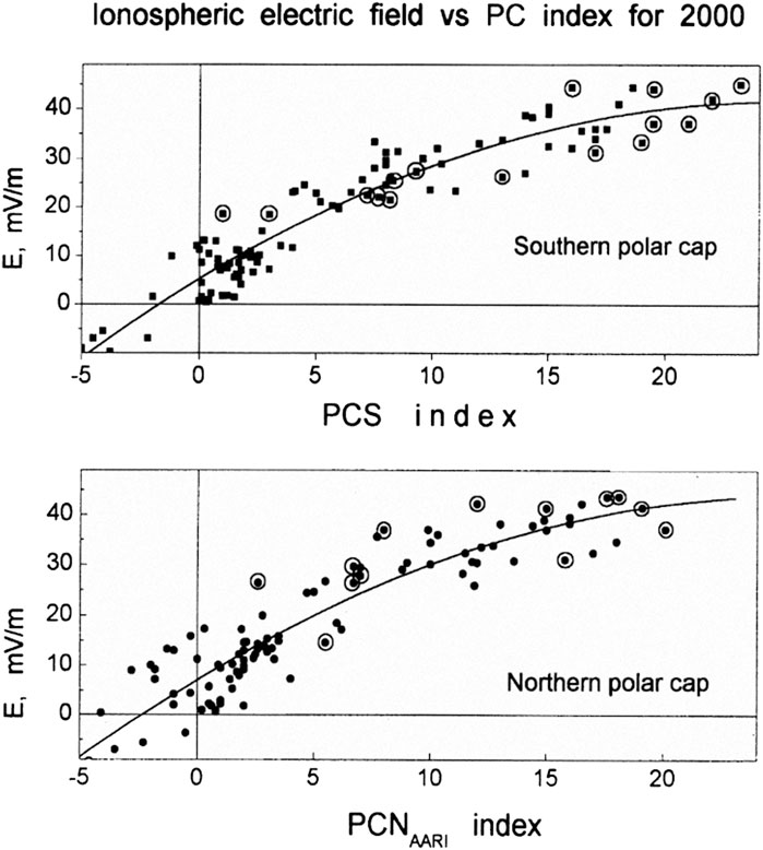
FIGURE 12. Relation between PC index and ionospheric electric field measured by DMSP spacecraft (h = 840 km) under conditions of high magnetic activity (Troshichev et al., 2000). Measurements during the days with powerful polar cap absorption are marked by points within the circles.

Good correlation (R = 0.88) between values of Φpc and PCN index was found by Bankov and Vassileva (2005) (with using data of measurements on board DMSP-F13 satellite in course 549 North Pole passes under various IMF conditions during spring of 1998), by Moon (2012) (correlation between Φpc and E_KL field, PCN index during 1996–2003 with peaks R = 0.82 in the equinoctial season), by Adhikari et al. (2017) (the relationships between Φpc and the solar wind parameters Vsw, B_X, B_Y, B_Z, the electric field E_KL, and geomagnetic indices PC, AL, SymH during the high intensive long duration auroral activity (HILDCAA) and supersubstorm (SSS) events). It was shown also (Chun et al., 1999, 2002) that PC index can serve as a proxy for the hemispheric Joule heating production rate.

Effect of the PC index “saturation” in response to solar wind electric field E_K was noted in (Nagatsuma, 2002; Troshichev et al., 2006; Stauning and Troshichev, 2008; Fiori et al., 2009). Term “saturation” in this context means that PC index practically stops to rise when E_KL field exceeds some critical value. The E_KL level that is necessary and sufficient for PC saturation was determined as 4 mV/m–5 mV/m by Nagatsuma (2002) and Troshichev et al. (2006), and as 2 mV/m by Fiori et al. (2009) (correlation between the PCN index and cross-polar cap velocity based on data of the Super DARN radars measurements).

Since the PC index is directly related to transpolar potential, saturation of PC index implies saturation of the cross-polar cap potential, which is commonly regarded, as a good proxy of the energy input into magnetosphere. In study (Ridley and Kihn, 2004) the assimilative mapping of ionosphere electrodynamics (AMIE) technique was used to calculate the cross polar cap potential and the polar cap electric field during 53 intervals with exceptionally large values of interplanetary electric field (10 mV/m) in 1997–2001. It was found that the transpolar potential estimated by linear extrapolation between the solar wind electric field and polar cap potential turned out to be overestimated as compared with the actually observed potential for values E_KL > 5–10 mV/m. Different mechanisms were proposed to explain this phenomenon (see reviews in Kivelson and Ridley, 2008; Borovsky et al., 2009); none of them was defined as the deciding factor.

In exploring the physical mechanism of the cross polar cap potential saturation, Kivelson and Ridley (2008) took into account the SuperDARN radar data and put forward the “transmitted potential” (E_KR function), which incorporates saturation of the cross polar potential. Analyses of relationship between the E_KR function and PC index (Gao et al., 2012a; Gao et al., 2012b; Gao, 2012) showed that correlation between the PC index and E_KR function is better than correlation between PC and E_KL field, especially when E_KR significantly differs from E_KL. The mechanisms, which are likely responsible for the discrepancy between the E_KL field and E_KR function effects were categorized by Gao (2012) as the following: 1) sources that effectively change the baseline values of magnetic field H and D components in deriving the PC index; 2) solar wind conditions that produced negative PC indices; 3) anomalous poleward excursions of the auroral oval; and 4) shifts of flow patterns arising from very strong IMF B_Y.

Thus, all above-listed analyses are evidence for relation of the cross polar cap voltage to the PC index value even though they are inconsistent in details. It should be noted in this connection that the PCN indices used in studies fulfilled before 2008 were derived by traditional method adopted in DMI (Vennerstrøm, 1991), which is strongly different from “unified method” (Troshichev et al., 2006) adopted in AARI for derivation of the PC index. The PCN indices, used in studies from 2008 to 2012, were, possibly, obtained by method described in (Stauning, 2011). After 2012 all PC indices, provided by the DTU Space Institute and AARI, were calculated by the “unified method” (Troshichev et al., 2006) approved by IAGA in 2013. Discrepancy of the described above results can account for difference in the methods of the PCN index calculation before 2012 and, correspondingly, for distinction of the used PCN indices.

7 PC index and the solar wind dynamic pressure (Pdyn) pulses

Interplanetary shocks denote the sudden and strong enhancements of solar wind dynamic pressure occurring when the high-speed solar plasma flows are propagated through space with low-speed plasma. Effects of the compression waves propagated in the magnetosphere are long known (Chapman and Ferraro, 1932). Impact of interplanetary shock on the Earth’s magnetosphere initiates sudden impulse (SI) in the geomagnetic field Evidences on influence of the sudden impulses on development of substorms and magnetic storms are ambiguous. On the one hand, it has long been known that power of magnetospheric disturbances (auroral particle precipitation, intensity of auroral electrojets, ring current injection rate and others) increases in correlation with the solar wind dynamic pressure (Boudouridis et al., 2003; Zhou et al., 2003; Gerard et al., 2004; Meurant et al., 2004). On the other hand, all these effects may be associated with the southward IMF fluctuations which are typical of the interplanetary shocks (Wang et al., 2003; Lee et al., 2004; Liou et al., 2004; Palmroth et al., 2004; Huang, 2005; Yue et al., 2010). Analyses of the PC index response to sudden changes in solar wind dynamic pressure have demonstrated a good correlation between the PC and E_KL field (Troshichev et al., 2007; Stauning and Troshichev, 2008) and between the PC and AL indices (Yue et al., 2010; Liou et al., 2017).

In study (Troshichev and Sormakov, 2019a) the solar wind dynamic pressure (Pdyn) pulses impacting on the magnetosphere were separated on the basis of solar wind parameters measured in the point of libration L1. Sudden pulses were identified as increase of the solar wind dynamic pressure (Pdyn) by value more than 10 nP within 5 min (http://omniweb.gsfc.nasa.gov). The actual moment of the SI contact with magnetosphere was defined by the appropriate sharp jump in the ground-based SymH index, the pulses power being expressed in the geomagnetic field units (nT). Only the events with the SI magnitude higher than 8 nT over the 8 min, starting against the background of steady quiet pressure level, were taken for the analysis (N = 108 for period 1998–2017).

The 1-min solar wind parameters, such as radial solar wind speed (Vx), vertical IMF component (Bz) and interplanetary electric field (E_KL), measured in the point of libration and reduced to the magnetopause, were regarded as indicators of the solar wind geoeffectiveness. The 1-min indices PCmean = (PCN + PCS)/2 and AL were examined as an indicator of the magnetospheric activity. Results of the analysis were presented as graphs summing up the time evolution of the ground-based SI events and indices PC, AL, on the one hand, and solar wind parameters Vx, E_KL, IMF Bz component, on the other hand, for the various conditions, such as: growing solar wind speed with Bz < 0 and with Bz > 0, steady solar wind speed with Bz < 0 and with Bz > 0, steady solar wind speed and Bz = 0, fluctuating solar wind speed and fluctuating Bz.

Figure 13 shows relationships between the SI magnitude and PC/AL indices for conditions of growing solar wind speed with Bz < 0 (A) and B_Z>0 (B), and for conditions of steady solar wind speed with Bz = 0 mV/m ± 1.5 mV/m (C), the SI contact with magnetosphere (T = 0) being identified by the appropriate jump in the ground-based SymH index. The results of the analysis demonstrate that the PC index correlates well with the pressure pulses only if the pulses are accompanied by corresponding jump in E_KL field. Under condition of the same SI magnitude (∆SymH∼30 nT) the intensity of magnetic disturbances (PC and AL indices) is maximal with growing solar wind velocity Vsw and southward IMF (Figure 15A), is insignificant with growing solar wind velocity Vsw and northward IMF (Figure 15B) and is negligible with steady Vsw and northward IMF (Figure 15C). One can see that intensity of magnetic disturbance is determined by the E_KL rise value in time of SI contact with magnetosphere. If the pressure pulses are not accompanied E_KL field rises, the magnetic disturbances are not appeared in polar cap (PC index) and in auroral zone (AL index).

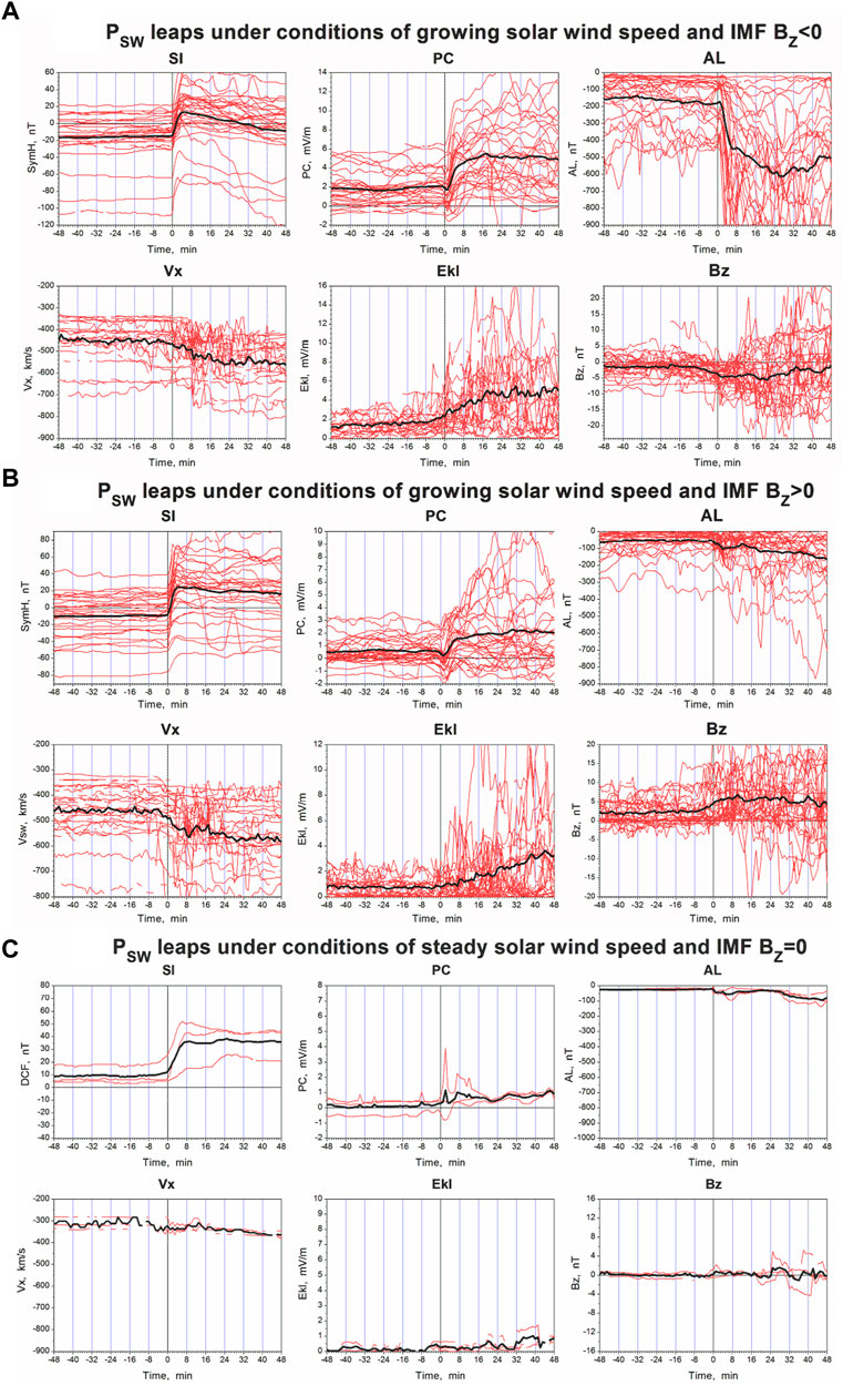
FIGURE 13. Time evolution of the actual ground-based SI events (identified with the Pdyn leaps), solar wind parameters Vsw, BZ, EKL and PC, AL indices under different conditions: (A) growing solar wind speed and negative IMF BZ values, (B) growing solar wind speed and positive IMF BZ values, (C) steady solar wind speed and BZ = 0 (Troshichev and Sormakov, 2019a).

Therefore, the pressure pulses themselves are not promote (or very insignificantly promote) the intensity of magnetic disturbances, which are regulated by E_KL field. This conclusion is fully agreed with inferences of Huang (2005) that “the PC index shows the same increase, no matter whether the IMF southward turning is accompanied by a solar wind pressure impulse or not” and Gao et al. (2012b) that “neither the solar wind dynamic pressure (Pdyn) nor jumps in Pdyn are found to directly contribute to the PC index”.

8 Discrepancy between the PCN and PCS indices: Role of the IMF BY component

The PC index value in the summer hemisphere (PCsummer) commonly exceeds the PC index value in the winter hemisphere (PCwinter). To illustrate this particularity in behavior of the PCN and PCS indices the difference between the monthly averaged definitive positive PCN and PCS values was estimated for each year during 1998–2018, the only positive PC indices being taken into account.

Figure 14 shows, as example, the courses of daily quantities of the definitive PCN (blue) and PCS (red) indices and their difference PCN-PCS (olive) in years of solar maximum (2000, 2011) and solar minimum (2008, 2019). One can see that PCN and PCS indices synchronously increase and decrease following the E_KL changes, the difference ΔPC = PCN-PCS being positive in May/June/July/August and negative in November/December/January/February, and close to zero in equinox. The value of ΔPC is the highest (up to 1 mV/m) in epochs of solar activity maximum and is minimal (<0.5 mV/m) in the quiet periods. It implies that difference between the daily quantities of PCsummer and PCwinter indices is caused by the solar wind influence.

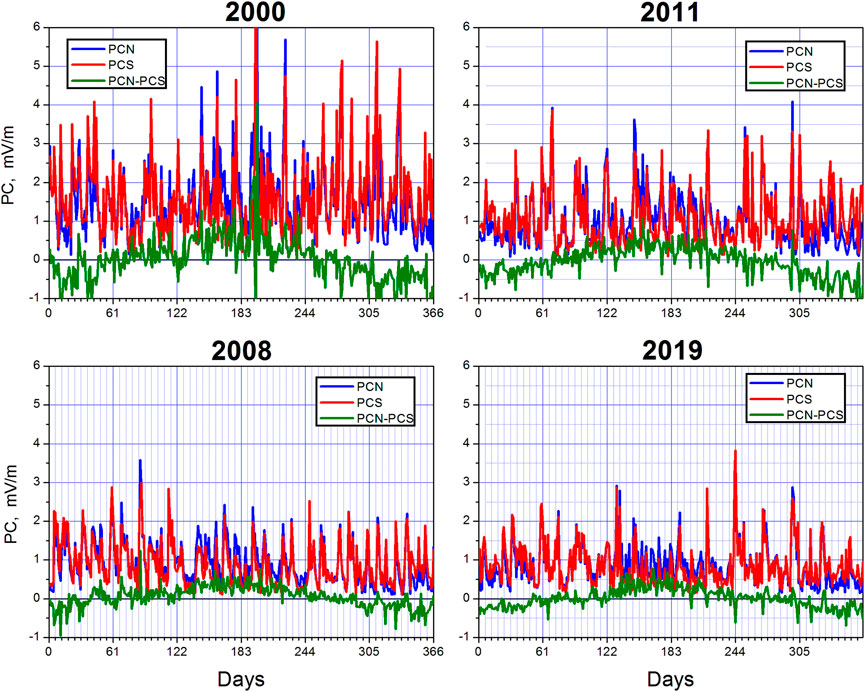
FIGURE 14. Courses of daily values of the PCN (blue) and PCS (red) indices and difference (PCN-PCS) (olive) in years of increased solar activity (2000, 2011) and in years of solar minimum (2008, 2019).

Regularity in occurrence and extent of the discrepancy ΔPC = PCN-PCS was studied basing on the hourly mean quantities of PCN and PCS indices and such solar wind parameters as E_KL field and B_Z, B_Y IMF components. The quantities ΔPC for 1997–2019 were examined separately for seasons North Summer, South Summer and Equinox for the following categories of corresponding PC indices: positive PCN and PCS indices (NpSp), negative PCN and PCS indices (NnSn), simultaneous PCN and PCS indices opposite in sign in the northern and southern polar caps (NSpn). The difference ΔPC = PCN-PCS was classified as positive (p) if PCN>PCS and negative (n) if PCN < PCS, with use of the following 5 gradations for positive value of ΔPC: p1 (0 mV/m–0.5 mV/m), p2 (0.5 mV/m–1 mV/m), p3 (1 mV/m–1.5 mV/m), p4 (1.5 mV/m–2 mV/m), p5 (>2 mV/m), and 5 corresponding gradations (n1, n2, n3, n4, n5) for negative values of ΔPC.

Total number of available hourly mean quantities used in the analysis was N = 189340, the main majority of data (∼75%) being related to positive PCN and PCS indices registered in both polar caps simultaneously (NpSp): the positive differences PCN-PCS>0 (NpSp, p) are typical for North Summer, the negative differences PCN-PCS<0 (NpSp, n) are typical of South Summer. The minimal number of data (∼7%) is related to the simultaneously registered negative PCN and PCS indices (NnSn). It should be remembered in this connection that negative PC index, caused by the northward IMF component in the limited near-pole region, can appear synchronously in summer and winter polar caps only under conditions of SPE events (Troshichev et al., 2022), during equinox in conditions of sufficient conductivity and extremely high northward IMF component.

Figure 15 shows dependency of ΔPC mean values (10 gradations) on E_KL mean values (A), IMF components BZ (B) and BY (C) for two ΔPC categories (NpSp, NSpn) in course of three seasons (Equinox, North summer, South summer) over 22 years, the category NnSn being excluded from examination in view of its scarce appearance. One can see (Figure 15A) that the positive PC values observed simultaneously in both polar caps (category NpSp) are typical of any E_KL values, the value of ΔPC (negative or positive) being increased with growth of E_KL. The PCN and PCS indices of contrary signs (category NSpn, second panel) appear mainly under conditions of low E_KL (0 mV/m–1 mV/m). Dependence of ΔPC on the southward Bzs (Figure 15B) is revealed only in case of positive PC indices (category NpSp) with correlation R = 0.58 for Equinox, R = 0.88 for North Summer and R = -0.54 for South Summer. For category NSpn dependence of ΔPC on B_Z is similar to dependence of ΔPC on E_KL, but it is observed under conditions of positive B_ZN IMF component. Figure 15C demonstrates evident dependence of ΔPC on the IMF B_Y component: the values ΔPC for categories NpSp and NSpn are positive (PCN>PCS) under conditions of positive B_Y and are negative (PCS < PCN) under conditions of negative B_Y component. The ΔPC values (positive or negative) are linearly increased with growth of the corresponding (positive or negative) IMF B_Y magnitude, the correlation between values ΔPC and By being larger than 0.95 for all categories of NpSp. Thus, the results, presented in Figure 15, are indicative of the E_KL field influences on ΔPC magnitude, not on sign of ΔPC. The B_Y IMF component seems to be the decisive factor determining the ΔPC sign, whereas the IMF B_Z component influences only value of ΔPC.

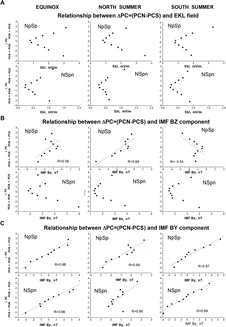
FIGURE 15. Relationships between the mean hourly values of ΔPC and E_KL field (A), IMF BZ component (B), IMF BY component (C) in equinox (left column), north summer (middle), south summer (right) for positive (NpSp), and contrary (NSpn) signs of PCN and PCS indices.

The mechanism of the B_Y IMF influence on the polar cap magnetic activity was examined in Section 2: appearance of BY FAC systems essentially distorts the regular DP2 convection patterns, the distortion effect being reversed in the northern and southern polar caps. Since direction of the field-aligned currents related to B_Y component is opposite in the northern and southern hemispheres, the sign of difference ΔPC = PCN-PCS turned out to be defined by sign of the B_Y IMF. The magnitude of discrepancy is determined by values of both B_Y and B_Z IMF components and their function, field E_KL = V_SW (B_Y²+B_Z)^1/2 sin²(θ/2), the extent of ΔPC being depended on ratio between the IMF B_Y and B_Z values, angle θ and season of year. Important role of the IMF B_Y component influence on the magnetosphere state was shown recently in (Tsyganenko and Andreeva, 2020).

9 Discussion

As this review shows, magnetic activity in polar caps is generated by separate FAC systems, which are related to solar wind parameters in different ways. The PC index characterizes the total solar wind impact on the magnetosphere exposed by “conventional” electric field E_KL, presenting the most geoeffective combination of the solar wind parameters. The E_KL influence is realized through R1 FAC system, which is positioned within the magnetosphere and always available irrespective of the IMF orientation. There are also independent BY and NBZ FAC systems, which are positioned in the day-time cusp region (BY) and in the sunlit area poleward from the cusp (NBZ) and related to processes occurring in the magnetosphere boundary layers. What are physical mechanisms providing influence of the E_KL field and separate IMF components on the magnetosphere?

Three concepts are applied at present to explain the solar wind–magnetosphere coupling. According to the best known concept put forward by Dungey (1961), the southward IMF carried by the solar wind is reconnected with the terrestrial magnetic field at the dayside magnetopause, where the geomagnetic field is northward. As a result, the terrestrial field lines merged with interplanetary field lines become open, and “interplanetary” electric field E = V x B_ZS is mapped along infinitely conducting magnetic field lines to the polar ionosphere. That provides the cross-polar cap electric potential, which is determined by intensity of the interplanetary electric field E and the merging line effective length l_eff at the dayside magnetopause: ΔV = l_effE (Vasyliunas, 1975). Concept of Dungey (1961) became at once very popular due to the fact that it was the only one during a long time idea, which accessibly explained the influence of the IMF direction (and intensity) on geomagnetic activity. However, there are numerous experimental evidences, which are not reconcilable with hypothesis of reconnection, such as turbulent properties of plasma inside the magnetosheath and rather common inconsistency between the required magnetic field directions outside (in solar wind) and inside of the boundary layer (in magnetosphere), the plasma sheet turbulence in the geomagnetic tail, occurrence of the “extraordinary” magnetic disturbances (substorms and storms) under conditions of the prolonged northward IMF, and so on. Moreover, according (Borovsky and Birn, 2014), the “interplanetary electric field” V_SWxB_SW does not control the rate of reconnection between IMF and geomagnetic field. It should be reminded also that the original Dungey’s concept does not even mention field-aligned currents since there was no any information about their existence in those times.

Another mechanism to couple the solar wind energy into the magnetosphere, known as a “viscous-like interaction”, was suggested by Axford and Hines (1961) and examined by Sonnerup (1980) and Heikkila (1990). According to this mechanism, the antisunward plasma convection on closed field lines is generated via the transfer of the solar wind momentum to the magnetospheric plasma across the magnetopause. It is commonly believed that a quasi-viscous interaction is determined by square of the solar wind speed v² (Sergeev and Kuznetsov, 1981; Boyle et al., 1997) or by combination of (n_SW^1/2v²) according to Newell et al. (2008). The viscous-like interaction is regarded as a little effective since it is responsible for not more than 15% of the polar cap voltage under the normal solar wind conditions (Reiff et al., 1981; Cowley, 1982; Boyle et al., 1997; Sonnerup et al., 2001). In addition, the studies (Newell and Meng, 1992; Wing et al., 2010) have demonstrated that all boundary layers in day-side magnetosphere are mapped at the region around the day-time cusp.

The third concept was put forward by Tverskoy (1969, 1972) and elaborated in (Antonova and Tverskoy, 1998; Antonova, 2002). According to this concept, the changes in distribution and value of geomagnetic field are related to changes of the value and distribution of plasma pressure in magnetosphere leading to formation of electric fields and field-aligned currents closing through the polar cap ionosphere. Thus, influence of the solar wind parameters at the magnetosphere dynamics is assigned to the plasma pressure changes within the magnetosphere under the solar wind influence. The Tverskoy’s concept (Tverskoy, 1969, 1972; Antonova and Tverskoy, 1998) appears to be very attractive, since it has predicted in fact the existence and distribution of the field-aligned currents consistent with the Region 1 and Region 2 currents, which were measured later on board Triad satellite (Iijima and Potemra, 1976a,b). Availability of the azimuthal plasma pressure gradients in magnetosphere was confirmed by measurements of particle fluxes in a wide energy range at a number of satellites (Xing et al., 2009).

The experimental results, presented in this review, demonstrate that both mechanisms, suggested by Dungey and by Tverskoy, are workable in the magnetosphere. Indeed, the concurrent availability of the R1 and NBZ FAC systems under conditions of the northward IMF (and superposed DP2+DP4 current systems in the sunlit ionosphere) is decisive evidence of simultaneous, but independent action of these mechanisms. Permanent availability of the R1 FAC system, which acts within the magnetosphere and responds appropriately to any changes of E_KL field (irrespective of polarity of the IMF B_Z and B_Y component), testifies in favor of the Tverskoy’s concept. Distinctive features of the BY and NBZ FAC spatial arrangement and their relation to processes in magnetosphere boundary layers are indicative of the magnetic interconnection mechanism of their origin (Dungey concept). In framework of Tverskoy’s concept the particular attention should be given to explanation of cardinal influence of the southward IMF component on the R1 FAC intensity. In other case we have to accept possibility of the specific SBZ FAC system appearance at the subsolar magnetosphere under conditions of southward IMF (B_Z < 0), which effect is added to effect of the R1 FAC system but remains indistinguishable on the total background.

At the same time we can ascertain a fact of absence of workable models capable to evaluate the efficiency of the solar wind–magnetosphere coupling in a real situation. In this context the PC index, linearly related to E_KL field, presents perhaps the only means to monitor on-line the geoeffectiveness of the solar wind-magnetosphere coupling. Because the strong distorted influence of the BY and NBZ FAC systems is displayed only in the well-conducted summer ionosphere, the PCwinter index should be regarded as a reliable indicator of the solar wind energy input into the magnetosphere.

10 Concluding remarks

The PC index has been introduced as a proxy of the solar wind energy that enters into the magnetosphere. The special “running QDC calculation” procedure made it possible to incorporate the effects of regular and irregular solar UV irradiance and the IMF sector structure effect into the level of reference (QDC). The procedure provides estimation the PC index value as an indicator of geoeffeciency of the solar wind (i.e., the E_KL power) coupling with the magnetosphere.

Impact of the solar wind electric field E_KL on the polar cap magnetic activity is realized through the R1 FAC system. The R1 FAC system is always in action, even under conditions of the strong northward IMF, the R1 FAC intensity in the undisturbed periods being dependent on conductivity of the polar cap ionosphere. Statistically justified relationships between the PC and E_KL values demonstrate that the PC index follows the E_KL field variations with a delay time ΔΤ∼12 min–20 min.

In spite of close correspondence between the E_KL field and PC index changes, correlation between the E_KL field and PC index is low or even negative in about 20% of time history. The matter is that the E_KL field is estimated by the solar wind parameters measured by the distant monitors far upstream of the magnetosphere (presented at site https://omniweb.gsfc.nasa.gov). In these cases the solar wind fixed by distant satellites did not encounter the magnetosphere. The PC index can be used to testify the actual solar wind geoeffectiveness.

A great advantage of the PC index application over other methods based on the satellite measurements is a permanent on-line availability of information on the magnetic activity in both northern and southern polar caps. A special procedure agreed by the Arctic and Antarctic Research Institute (AARI) and Space Institute of the Danish Technical University (DTUSpace) ensures the permanent calculation of the unified PC index in quasi-real time.

Author contributions

The author confirms being the sole contributor of this work and has approved it for publication.

Acknowledgments

The definitive PCN and PCS indices are presented at websites http://pcindex.org and http://isgi.unistra.fr. The solar wind and IMF data were obtained from the GSFC/SPDYNF OMNI/Web interface at http://omniweb.gsfc.nasa.gov. The AE and Dst indices were provided by WDC-C2 Kyoto (http://wdc.kugi.kyoto-u.ac.jp/wdc/cresample.html). The Solar UV Irradiance data are presented on site (https://lasp.colorado.edu/lisird/data/lasp_gsfc_composite_ssi/). Information on ICME and SIR(CIR)-driven magnetic storms was taken from Catalogue of ICMEs [I. Richardson and H.Cane, 2015], and List of Stream Interaction Regions Observed by STEREO A/B [L.Jian, 2015].

Conflict of interest

The author declares that the research was conducted in the absence of any commercial or financial relationships that could be construed as a potential conflict of interest.

Publisher’s note

All claims expressed in this article are solely those of the authors and do not necessarily represent those of their affiliated organizations, or those of the publisher, the editors and the reviewers. Any product that may be evaluated in this article, or claim that may be made by its manufacturer, is not guaranteed or endorsed by the publisher.

References

Adhikari, B., Baruwal, P., and Chapagain, N. P. (2017). Analysis of supersubstorm events with reference to polar cap potential and polar cap index. Earth Space Sci. 4, 2–15. doi:10.1002/2016EA000217
Akasofu, S-I. (1979). Interplanetary energy flux associated with magnetospheric substorms. Planet. Space Sci. 27, 425–431. doi:10.1016/0032-0633(79)90119-3
Anderson, B. J., Korth, H., Waters, C. L., Green, D. L., and Stauning, P. (2008). Statistical Birkeland current distributions from magnetic field observations by the Iridium constellation. Ann. Geophys. 26, 671–687. doi:10.5194/angeo-26-671-2008
Antonova, E. E., and Tverskoy, B. A. (1998). On the nature of electric fields in the Earth’s inner magnetosphere. Geomagn. Aeron. Int. 1, 9–21.
Antonova, E. E., Kirpichev, I. P., and Stepanova, M. V. (2006). Field-aligned current mapping and the problem of the generation of magnetospheric convection. Adv. Space Res. 38, 1637–1641. doi:10.1016/j.asr.2005.09.042
Antonova, E. E., Kirpichev, I. P., Vovchenko, V. V., Stepanova, M. V., Riazantseva, M. O., Pulinets, M., et al. (2013). Characteristics of plasma ring, surrounding the Earth at geocentric distances ∼7–10RE, and magnetospheric current systems. J. Atmos. Sol. Terr. Phys. 99, 85–91. doi:10.1016/j.jastp.2012.08.013
Antonova, E. E., Kirpichev, I. P., and Stepanova, M. V. (2014). Plasma pressure distribution in the surrounding the Earth plasma ring and its role in the magnetospheric dynamics. J. Atmos. Sol. Terr. Phys. 115, 32–40. doi:10.1016/j.jastp.2013.12.005
Antonova, E. E., Stepanova, M., Kirpichev, I. P., Ovchinnikov, I. L., Vorobjev, V. G., Yagodkina, O., et al. (2018). Structure of magnetospheric current systems and mapping of high latitude magnetospheric regions to the ionosphere. J. Atmos. Solar-Terrestrial Phys. 177, 103–114. doi:10.1016/j.jastp.2017.10.013
Antonova, E. E. (2002). Magnetostatic equilibrium and turbulent transport in Earth’s magnetosphere: A review of experimental observation data and theoretical approach. Geom. Aeron. Int. 3, 117–130.
Armstrong, J. C., and Zmuda, A. J. (1970). Field-aligned current at 1100 km in the auroral region measured by satellite. J. Geophys. Res. 75, 7122–7127. doi:10.1029/ja075i034p07122
Axford, W. I., and Hines, C. O. (1961). A unifying theory of high-latitude geophysical phenomena and geomagnetic storms. Can. J. Phys. 39, 1433–1464. doi:10.1139/p61-172
Bankov, L. G., and Vassileva, A. K. (2005). “Polar cap index versus polar cap potential variations as a subject of the solar wind-magnetosphere interactions,” in Scientific Conference “SPACE, ECOLOGY, SAFETY”, Varna, Bulgaria, June 10–13, 2005.
Borovsky, J. E., and Birn, J. (2014). The solar-wind electric field does not control the dayside reconnection rate. J. Geophys. Res. Space Phys. 119, 751–760. doi:10.1002/2013ja019193
Borovsky, J. E., Lavraud, B., and Kuznetsova, M. M. (2009). Polar cap potential saturation, dayside reconnection, and changes to the magnetosphere. J. Geophys. Res. 114, A03224. doi:10.1029/2009JA014058
Boudouridis, A., Zesta, E., Lyons, R., Anderson, P. C., and Lummerzheim, D. (2003). Effect of solar wind pressure pulses on the size and strength of the auroral oval. J. Geophys. Res. 108, 8012. doi:10.1029/2002ja009373
Boyle, C. B., Reiff, P. H., and Hairston, M. R. (1997). Empirical polar cap potentials. J. Geophys. Res. 102, 111–125. doi:10.1029/96JA01742
Bythrow, P. F., and Potemra, T. A. (1983). The relationship of total Birkeland currents to the merging electric field. Geophys. Res. Lett. 10, 573–576. doi:10.1029/gl010i007p00573
Chan, F. C., and Russel, C. T. (2000). “Statistical characteristics of field-aligned currents in the Earth’s inner magnetosphere,” in Magnetospheric current systems. Editors S. Ohtani, R. Fujii, M. Hesse, and R. Lysak (Washington: AGU), 237–243.
Chapman, S., and Ferraro, V. C. (1932). A new theory of magnetic storms: I. Initial phase. J. Geophys. Res. 37, 147–156. doi:10.1029/te037i002p00147
Chun, F. K., Knipp, D. J., McHarg, M. G., Lu, G., Emery, B. A., Vennerstrøm, S., et al. (1999). Polar cap index as a proxy for hemispheric Joule heating. Geophys. Res. Lett. 26 (8), 1101–1104. doi:10.1029/1999gl900196
Chun, F. K., Knipp, D. J., McHarg, M. G., Lacey, J. R., Lu, G., and Emery, B. A. (2002). Joule heating patterns as a function of polar cap index. J. Geophys. Res. 107 (7), 1119. doi:10.1029/2001JA000246
Cowley, S. W. H. (1982). The causes of convection in the earth's magnetosphere: A review of developments during the IMS. Rev. Geophys. 20, 531–565. doi:10.1029/rg020i003p00531
Despirak, I., Lubchich, A., and Kleimenova, N. (2016). Comparison of substorms near two solar cycle maxima: (1999-2000 and 2012-2013). Sun Geosph. 11 (2), 101–106.
Dungey, J. W. (1961). Interplanetary magnetic field and the auroral zones. Phys. Rev. Lett. 6, 47–48. doi:10.1103/physrevlett.6.47
Fairfield, D. H., and Mead, G. D. (1975). Magnetospheric mapping with a quantitative geomagnetic field model. J. Geophys. Res. 80, 535–542. doi:10.1029/ja080i004p00535
Fiori, R. A. D., Koustov, A. V., Boteler, D., and Makarevich, R. A. (2009). PCN magnetic index and average convection velocity in the polar cap inferred from SuperDARN radar measurements. J. Geophys. Res. 114, A07225. doi:10.1029/2008JA013964
Frank, L. A., and Garnett, D. A. (1971). Distribution of plasmas and electric fields over the auroral zones and polar caps. J. Geophys Res. 76, 49–55.
Friis-Christensen, E., and Wilhjelm, J. (1975). Polar cap currents for different directions of the interplanetary magnetic field in the Y-Z plane. J. Geophys. Res. 80, 1248–1260. doi:10.1029/ja080i010p01248
Fukushima, N. (1969). Equivalence in ground magnetic effect of Chapman-Vestine’s and Birkeland-Alfven’s electric current systems for polar magnetic storms. Rep. Ion. Space Res. Jpn. 23, 219–227.
Gao, Y., Kivelson, M. G., and Walker, R. J. (2012a). The linear dependence of polar cap index on its controlling factorsin solar wind and magnetotail. J. Geophys. Res. 117, A05213. doi:10.1029/2011JA017229
Gao, Y., Kivelson, M. G., Ridley, A. J., Weygand, J. M., and Walker, R. J. (2012b). Utilizing the polar cap index to explore strong driving of polar cap dynamics. J. Geophys. Res. 117, A07213. doi:10.1029/2011JA017087
Gao, Y. (2012). On anomalous departures from a linear relation between the polar cap index and its controlling factors in solar wind and magnetotail. J. Geophys. Res. 117, A06201. doi:10.1029/2012JA017721
Gerard, J. C., Hubert, B., Grard, A., Meaurant, M., and Mende, S. B. (2004). Solar wind control of auroral substorm onset locations observed with the IMAGE-FUV imagers. J. Geophys. Res. 109, A03208. doi:10.1029/2003JA010129,
Gizler, V. A., Semenov, V. S., and Troshichev, O. A. (1979). Electric fields and currents in the ionosphere generated by field-aligned currents observed by TRIAD. Planet. Space Sci. 27, 223–231. doi:10.1016/0032-0633(79)90064-3
Green, D. L., Waters, C. L., Anderson, B. J., and Korth, H. (2009). Seasonal and interplanetary magnetic field dependence of the field-aligned currents for both Northern and Southern Hemispheres. Ann. Geophys. 27, 1701–1715. doi:10.5194/angeo-27-1701-2009
Heikkila, W. J. (1990). Magnetic reconnection, merging, and viscous interaction in the magnetosphere. Space Sci. Rev. 53, 1. doi:10.1007/bf00217427
Heppner, J. P., Stolarik, J. D., and Wescott, E. M. (1971). Electric-field measurements and the identification of currents causing magnetic disturbances in the polar cap. J. Geophys. Res. 76, 6028–6053. doi:10.1029/ja076i025p06028
Huang, C. S. (2005). Variations of polar cap index in response to solar wind changes and magnetospheric substorms. J. Geophys. Res. 110, A01203. doi:10.1029/2004ja010616,
IAGA Resolution (2021). The IAGA Business Meeting. Available at: www.iaga-aiga.org/resolutions/resolution-no-2-2021-polar-cap-pc-index/.
IAGA Resolutions (2013). “Resolution No. 3: Polar Cap (PC) index,” in XXII Assembly of International Geomagnetism and Aeronomy Association, Merida, Mexico, August 25-31, 2013. Available at: http://www.iaga-aiga.org/resolutions.
Iijima, T., and Potemra, T. A. (1976a). The amplitude distribution of field-aligned currents at northern high latitudes observed by Triad. J. Geophys. Res. 81, 2165–2174. doi:10.1029/ja081i013p02165
Iijima, T., and Potemra, T. A. (1976b). Field-aligned currents in the day-side cusp observed by Triad. J. Geophys. Res. 81, 5971–5979. doi:10.1029/ja081i034p05971
Iijima, T., and Potemra, T. A. (1982). The relationship between interplanetary quantities and Birkeland current densities. Geophys. Res. Lett. 4, 442–445. doi:10.1029/gl009i004p00442
Iijima, T., and Shibaji, T. (1987). Global characteristics of northward IMF-associated (NBZ) field-aligned currents. J. Geophys. Res. 92, 2408–2424. doi:10.1029/ja092ia03p02408
Iijima, T., Fujii, R., Potemra, T. A., and Saflekos, T. A. (1978). Field-aligned currents in the south polar cusp and their relationship to the interplanetary magnetic field. J. Geophys. Res. 83, 5595–5603. doi:10.1029/ja083ia12p05595
Iijima, T., Potemra, T. A., Zanetti, L. J., and Bythrow, P. F. (1984). Large-scale birkeland currents in the day-side polar region during strongly northward IMF: A new birkeland current system. J. Geophys. Res. 89, 7441–7452. doi:10.1029/ja089ia09p07441
Iijima, T., Potemra, T. A., and Zanetti, L. J. (1997). Contribution of pressure gradients to the generation of dawnside region 1 and region 2 currents. J. Geophys. Res. 102, 27069–27081. doi:10.1029/97ja02462
Iwasaki, N. (1971). Localized abnormal geomagnetic disturbances near the geomagnetic pole and simultaneous ionospheric variations. Rep. Ion. Space Res. Jpn. 25, 163–186.
Kamide, Y., and Baumjohann, W. (1993). Magnetosphere-ionosphere coupling. Berlin-Heidelberg-New York: Springer-Verlag, 178.
Kamide, Y., and Matsushita, S. (1979). Simulation studies of ionospheric electric fields and currents in relation to field-aligned currents: 1 quiet periods, 2 substorms. J. Geophys. Res. 84, 4083–4098. doi:10.1029/ja084ia08p04083
Kan, J. R., and Lee, L. C. (1979). Energy coupling function and solar wind-magnetosphere dynamo. Geophys. Res. Lett. 6, 577–580. doi:10.1029/gl006i007p00577
Khan, P. A., Tripathi, S. C., Troshichev, O. A., Waheed, M. A., Aslam, A. M., and Gwal, A. K. (2013). Solar transients disturbing the terrestrial magnetic environment at higher latitudes. Astrophys. Space Sci. 349, 647–656. doi:10.1007/s10509-013-1661-5
King, J. H., and Papitashvili, N. E. (2005). Solar wind spatial scales in and comparisons of hourly Wind and ACE plasma and magnetic field data. J. Geophys. Res. 110, A02104. doi:10.1029/2004JA010649
Kivelson, M. G., and Ridley, A. J. (2008). Saturation of the polar cap potential: Inference from Alfven wing arguments. J. Geophys. Res. 113, A05214. doi:10.1029/2007JA012302
Kullen, A., Karlsson, T., Cumnock, J. A., and Sundberg, T. (2010). Occurrence and properties of substorms associated with pseudobreakups. J. Geophys. Res. 115, A12310. doi:10.1029/2010JA015866
Kuznetsov, B. M., and Troshichev, O. A. (1977). On the nature of polar cap magnetic activity during undisturbed periods. Planet. Space Sci. 25, 15–21. doi:10.1016/0032-0633(77)90113-1
Langel, R. A. (1975). Relation of variations in total magnetic field at high latitude with the parameters of the interplanetary magnetic field and withDP2 fluctuations. J. Geophys. Res. 80, 1261–1270. doi:10.1029/ja080i010p01261
Laundal, K. M., and Toresen, M. (2018). pyAMPS. Available at: https://github.com/klaundal/pyAMPS.
Laundal, K. M., Finlay, C. C., Olsen, N., and Reistad, J. P. (2018). Solar wind and seasonal influence on ionospheric currents from Swarm and CHAMP measurements. J. Geophys. Res. Space Phys. 123, 4402–4429. doi:10.1029/2018JA025387
Lee, D. Y., Lyons, L. R., and Yumoto, K. (2004). Sawtooth oscillations directly driven by solar wind dynamic pressure enhancements. J. Geophys. Res. 109, A04202. doi:10.1029/2003JA010246
Liou, K., Carbary, J. F., Newell, P. T., Meng, C.-I., and Rasmussen, O. (2003). Correlation of auroral power with the polar cap index. J. Geophys. Res. 108 (A3), 1108. doi:10.1029/2002ja009556
Liou, K., Newell, P. T., Meng, C-I., Wu, C.-C., and Lepping, R. P. (2004). On the relationship between shock-induced polar magnetic bays and solar wind parameters. J. Geophys. Res. 109, A06306. doi:10.1029/2004JA010400
Liou, K., Sotirelis, T., and Gjerloev, J. (2017). Statistical study of polar negative magnetic bays driven by interplanetary fast-mode shocks. JGR. Space Phys. 122, 7463–7472. doi:10.1002/2017JA024465
Logachev Yu, I., Bazilevskaya, G. A., Vashenyuk, E. V., Daibog, E. I., Ishkov, V. N., Lazutin, L. L., et al. (2016). Catalog of Solar Proton Events in the 23rd Cycle of Solar Activity (1996–2008). ESDBrepository, GC RAS, Moscow. doi:10.2205/ESDB-SAD-P-001-RU
Logachev Yu, I., Bazilevskaya, G. A., Vlasova, N. A., Ginzburg, E. A., Ishkov, V. N., Lazutin, L. L., et al. (2022). Catalog of solar proton events in the 24th cycle of solar activity (2009–2019). ESDB repository, GC RAS, Moscow. doi:10.2205/ESDB-SAD-008
Lukianova, R., Troshichev, O., and Lu, G. (2002). The polar cap magnetic activity indices in the southern (PCS) and northern (PCN) polar caps: consistency and discrepancy. Geophys. Res. Lett. 29, 26-1–26-4. doi:10.1029/2002gl015179
Maezawa, K. (1976). Magnetospheric convection induced by the positive and negative Z components of the interplanetary magnetic field: quantitative analysis using polar cap magnetic records. J. Geophys. Res. 81, 2289–2303. doi:10.1029/ja081i013p02289
Mansurov, S. M. (1969). A new evidence for relationship between the space and Earth magnetic fields. Geomagn. Aeron. 9, 768–770. (in Russian).
Matsushita, S., Tarpley, J. D., and Campbell, W. H. (1973). IMF sector structure effects on the quiet geomagnetic field. Radio Sci. 8, 963–972. doi:10.1029/rs008i011p00963
McCreadie, H., and Menvielle, M. (2010). The PC index: review of methods. Ann. Geophys. 28, 1887–1903. doi:10.5194/angeo-28-1887-2010
McDiarmid, I. B., Burrows, J. R., and Wilson, M. D. (1977). Reverse polarity field-aligned currents at high latitudes. J. Geophys. Res. 82, 1513–1518. doi:10.1029/ja082i010p01513
McDiarmid, I. B., Burrows, J. R., and Wilson, M. D. (1978). Magnetic field perturbations in the dayside cleft and their relationship to the IMF. J. Geophys. Res. 83, 5753–5756. doi:10.1029/ja083ia12p05753
McDiarmid, I. B., Burrows, J. R., and Wilson, M. D. (1979). Large-scale magnetic field perturbations and particle measurements at 1400 km on the dayside. J. Geophys. Res. 84, 1431. doi:10.1029/ja084ia04p01431
Meurant, M., Gerard, J., Blockx, C., Hubert, B., and Coumans, V. (2004). Propagation of electron and proton shock-induced aurora and the role of the interplanetary magnetic field and solar wind. J. Geophys. Res. 109, A10210. doi:10.1029/2004JA010453
Moon, G-H. (2012). Estimation of polar cap potential and the role of PC index. J. Astron. Space Sci. 29 (3), 259–267. doi:10.5140/JASS.2012.29.3.259
Mozer, F. S., Gonzales, W. D., Bogott, F., Kelley, M. C., and Schutz, S. (1974). High-latitude electric fields and the three-dimensional interaction between the interplanetary and terrestrial magnetic fields. J. Geophys. Res. 79, 56–63. doi:10.1029/ja079i001p00056
Nagata, T., and Kokubun, S. (1962). An additional geomagnetic daily variation (Sqp field) in the polar region on a geomagnetically quiet day. Rep. Ion. Space Res. Jpn. 16, 256–274.
Nagatsuma, T. (2002). Saturation of polar cap potential by intense solar wind electric fields. Geophys. Res. Lett. 29 (10), 62-1–62-4. doi:10.1029/2001GL014202
Newell, P. T., and Meng, C. I. (1992). Mapping the dayside ionosphere to the magnetosphere according to particle precipitation characteristics. Geophys. Res. Lett. 19, 609–612. doi:10.1029/92gl00404
Newell, P. T., Sotirelis, T., Liou, K., and Rich, F. J. (2008). Pairs of solar wind-magnetosphere coupling functions: Combining a merging term with a viscous term works best. J. Geophys. Res. 113, A04218. doi:10.1029/2007JA012825
Nielsen, J. B., and Willer, A. N. (2019). Restructuring and harmonizing the code used to calculate the definitive polar cap index. Copenhagen: Report from DTU Space. Available at: https://tinyurl.com/sx3g5t5.
Nishida, A., and Maezawa, K. (1971). Two basic modes of interaction between the solar wind and the magnetosphere. J. Geophys. Res. 76, 2254–2264. doi:10.1029/ja076i010p02254
Nishida, A. (1968a). GeomagneticDp2 fluctuations and associated magnetospheric phenomena. J. Geophys. Res. 73, 1795–1803. doi:10.1029/ja073i005p01795
Nishida, A. (1968b). Coherence of geomagnetic DP2 fluctuations with interplanetary magnetic variations. J. Geophys. Res. 73, 5549–5559. doi:10.1029/ja073i017p05549
Obayashi, T. (1967). in The interaction of solar plasma with geomagnetic field, disturbed conditions. Editors J. W. King, and W. S. Newman (N.Y.), 107. Solar terrestrial physics.
Ohtani, S., Potemra, T. A., Newell, P. T., Zanetti, L. J., Iijima, T., Watanabe, M., et al. (1995). Simultaneous prenoon and postnoon observations of three field-aligned current systems from Viking and DMSP-F7. J. Geophys. Res. 100, 119–136. doi:10.1029/94ja02073
Palmroth, M., Pulkkinen, T. I., Janhunen, P., McComas, D. J., Smith, C. W., and Koskinen, H. E. J. (2004). Role of solar wind dynamic pressure in driving ionospheric Joule heating. J. Geophys. Res. 109, A11302. doi:10.1029/2004JA010529
Potemra, T. A. (1978). Observation of Birkeland currents with the TRIAD satellite. Astrophys. Space Sci. 58, 207–226. doi:10.1007/bf00645387
Reiff, P. H., and Luchmann, J. G. (1986). “Solar wind control of the polar-cap voltage,” in Solar wind – magnetosphere coupling. Editors Y. Kamide, and J. A. Slavin (Tokyo), 453–476. Terra Sci.
Reiff, P. H., Spiro, R. W., and Hill, T. W. (1981). Dependence of polar cap potential drop on interplanetary parameters. J. Geophys. Res. 86, 7639–7648. doi:10.1029/ja086ia09p07639
Ridley, A. J., and Kihn, E. A. (2004). Polar cap index comparisons with AMIE cross polar cap potential, electric field, and polar cap area. Geophys. Res. Lett. 31, L07801. doi:10.1029/2003GL019113
Saflekos, N. A., and Potemra, T. A. (1980). The orientation of Birkeland current sheets in the dayside polar region and its relationship to the IMF. J. Geophys. Res. 85, 1987–1994. doi:10.1029/ja085ia05p01987
Sergeev, V. A., and Kuznetsov, B. M. (1981). Quantitative dependence of the polar cap electric field on the IMF BZ component and solar wind velocity. Planet. Space Sci. 29, 205–213. doi:10.1016/0032-0633(81)90034-9
Sonnerup, B. U. O., Siebert, K. D., White, W. W., Meimer, D. R., Maynard, N. C., Schoendorf, J. A., et al. (2001). Simulations of the magnetosphere for zero interplanetary magnetic field: The ground state. J. Geophys. Res. 106, 29419–29434. doi:10.1029/2001ja000124
Sonnerup, B. U. O. (1980). Theory of the low-latitude boundary layer. J. Geophys. Res. 85, 2017–2026. doi:10.1029/ja085ia05p02017
Stauning, P., and Troshichev, O. A. (2008). Polar cap convection and PC index during sudden changes in solar wind dynamic pressure. J. Geophys. Res. 113, A08227. doi:10.1029/2007JA012783
Stauning, P. (2011). Determination of the quiet daily geomagnetic variations for polar regions. J. Atmos. Sol. Terr. Phys. 73, 2314–2330. doi:10.1016/j.jastp.2011.07.004
Svalgaard, L. (1968). Sector structure of the interplanetary magnetic field and daily variation of the geomagnetic field at high latitudes. Charlottenlund: Det Danske meteorologiske institute. preprint R-6.
Takalo, J., and Timonen, J. (1998). On the relation of the AE and PC indices. J. Geophys. Res. 103, 29393–29398. doi:10.1029/98ja02390
Troshichev, O. A., and Andrezen, V. G. (1985). The relationship between interplanetary quantities and magnetic activity in the southern polar cap. Planet. Space Sci. 33, 415–419. doi:10.1016/0032-0633(85)90086-8
Troshichev, O., and Janzhura, A. (2012). Space weather monitoring by ground-based means: PC index. Berlin, Heidelberg: Springer-Verlag, 288. doi:10.1007/978-3-642-16803-1
Troshichev, O. A., and Sormakov, D. A. (2015). PC index as a proxy of the solar wind energy that entered into the magnetosphere: (2) relation to the interplanetary electric field EKL. Earth Planets Space 67, 170. doi:10.1186/s40623-015-0338-4
Troshichev, O. A., and Sormakov, D. A. (2019a). PC index as a proxy of the solar wind energy that entered into the magnetosphere: 4. Relationship between the solar wind dynamic pressure (PDYN) pulses and PC, AL indices. J. Atmos. Sol. Terr. Phys. 182, 200–210. doi:10.1016/j.jastp.2018.12.001
Troshichev, O. A., and Sormakov, D. A. (2019b). PC index as a proxy of the solar wind energy that entered into the magnetosphere: (5) verification of the solar wind parameters presented at OMNI website. J. Atmos. Sol. Terr. Phys. 196, 105147. doi:10.1016/j.jastp.2019.105147
Troshichev, O. A., and Tsyganenko, N. A. (1979). Correlation relationships between variations of IMF and magnetic disturbances in the polar cap. Geomagn Res. 25, 47–59. (in Russian).
Troshichev, O. A., Dmitrieva, N. P., and Kuznetsov, B. M. (1979a). Polar cap magnetic activity as a signature of substorm development. Planet. Space Sci. 27, 217–221. doi:10.1016/0032-0633(79)90063-1
Troshichev, O. A., Gizler, V. A., Ivanova, I. A., and Merkurieva, A. Yu. (1979b). Role of field-aligned currents in generation of high latitude magnetic disturbances. Planet. Space Sci. 27, 1451–1459. doi:10.1016/0032-0633(79)90091-6
Troshichev, O. A., Andrezen, V. G., Vennerstrøm, S., and Friis-Christensen, E. (1988). Magnetic activity in the polar cap – a new index. Planet. Space Sci. 36, 1095–1102. doi:10.1016/0032-0633(88)90063-3
Troshichev, O. A., Hayakawa, H., Matsuoka, A., Mukai, T., and Tsuruda, K. (1996). Cross polar cap diameter and voltage as a function of PC index and interplanetary quantities. J. Geophys. Res. 101, 13429–13435. doi:10.1029/95ja03672
Troshichev, O. A., Lukianova, R., Papitashvili, V. O., Rich, F. J., and Rasmussen, O. (2000). Polar cap index (PC) as a proxy for ionospheric electric field in the near-pole region. Geophys. Res. Lett. 27, 3809–3812. doi:10.1029/2000gl003756
Troshichev, O., Janzhura, A., and Stauning, P. (2006). Unified PCN and PCS indices: Method of calculation, physical sense and dependence on the IMF azimuthal and northward components. J. Geophys. Res. 111, A05208. doi:10.1029/2005JA011402
Troshichev, O., Janzhura, A., and Stauning, P. (2007). Magnetic activity in the polar caps: Relation to sudden changes in the solar wind dynamic pressure. J. Geophys. Res. 112. doi:10.1029/2007JA012369
Troshichev, O. A., Podorozhkina, N. A., and Janzhura, A. S. (2011a). Invariability of relationship between the polar cap magnetic activity and geoeffective interplanetary electric field. Ann. Geophys. 29, 1479–1489. doi:10.5194/angeo-29-1479-2011
Troshichev, O. A., Podorozhkina, N. A., Sormakov, D. A., and Janzhura, A. S. (2014). PC index as a proxy of the solar wind energy that entered into the magnetosphere: Development of magnetic substorms. J. Geophys. Res. Space Phys. 119, 6521–6540. doi:10.1002/2014JA019940
Troshichev, O. A., Dolgacheva, S. A., Stepanov, N. A., and Sormakov, D. A. (2021). The PC index variations during 23/24 solar cycles: relation to solar wind parameters and magnetospheric disturbances. JGR. Space Phys. 126. doi:10.1029/2020JA028491
Troshichev, O. A., Dolgacheva, S. A., and Sormakov, D. A. (2022). Invariability of relationships between the solar wind electric field EKL and the magnetic activity indices PC, AL and Dst. J. Atmos. Sol. Terr. Phys., 235, 105894, doi:10.1016/j.jastp.2022.105894
Troshichev, O. A. (1975). “Magnetic disturbances in polar caps and parameters of solar wind,” in Substorms and magnetospheric disturbances (Leningrad: Nauka), 66–83. (in Russian).
Troshichev, O. A. (1982). Polar magnetic disturbances and field-aligned currents. Space Sci. Rev. 32, 275–360. doi:10.1007/bf00167945
Troshichev, O. A. (1984). “Solar wind control of electric fields and currents in the magnetosphere and ionosphere,” in Proc. Conf. Achievements IMS, Graz, Austria, June 26–28, 1984, 407–416.
Troshichev, O. A. (2017). Polar cap magnetic activity (PC index) and space weather monitoring. Saarbrucken: Editions universitaires europeennes, 140.
Tsyganenko, N. A., and Andreeva, V. A. (2020). Magnetospheric “penetration” of IMF viewed through the lens of an empirical RBF modeling. JGR. Space Phys. 125, e2019JA027439. doi:10.1029/2019JA027439
Tsyganenko, N. A. (1996). “Effects of the solar wind conditions on the global magnetospheric configuration as deduced from data-based field models,” in Proceedings of the Third International Conference on Substorms (ICS-3), Versailles, France, May 12–17, 1996 (Eur Space Agency Spec. Publication, ESA-SP) Vol. 389, 181–185.
Tsyganenko, N. A. (2002). A model of the near magnetosphere with a dawn-dusk asymmetry 2. Parameterization and fitting to observations. J. Geophys. Res. 107 (A7), SMP 10-11–SMP 10-17. doi:10.1029/2001JA000220
Tverskoy, B. A. (1969). On electric fields in the Earth’s magnetosphere. Dokl. Akad. Nauk. USSR 188, 575–578. (in Russian).
Tverskoy, B. A. (1972). “Electric fields in the magnetosphere and the origin of trapped radiation,”. Editor E. R. Dyer (Dordrecht, Holland), 297–317. Solar-Terrestrial Physics.
Vanjan, L. L., and Osipova, I. L. (1975). Electric conductivity of polar ionosphere. Geomagn. Aeron. 15, 847.
Vassiliadis, D., Angelopoulos, V., Baker, D. N., and Klimas, A. J. (1996). The relation between the northern polar cap and auroral electrojet geomagnetic indices in the wintertime. Geophys. Res. Lett. 23, 2781–2784. doi:10.1029/96gl02575
Vasyliunas, V. M. (1975). Theoretical models of magnetic field line merging. Rev. Geophys. 3, 303. doi:10.1029/rg013i001p00303
Vennerstrøm, S., Friis-Christensen, E., Troshichev, O. A., and Andrezen, V. G. (1991). Comparison between the polar cap index PC and the auroral electrojet indices AE, AL and AU. J. Geophys. Res. 96, 101. doi:10.1029/90ja01975
Vennerstrøm, S. (1991). The geomagnetic activity index PC. PhD Thesis. Copenhagen: Danish Meteorological Institute, 105. Scientific Report 91-3. Available at: https://www.dmi.dk/fileadmin/user_upload/Rapporter/SR/1991/sr91-3.pdf.
Vokhmyanin, M. V., Stepanov, N. A., and Sergeev, V. A. (2019). On the evaluation of data quality in the OMNI interplanetary magnetic field database. Space weather. 17, 476–486. doi:10.1029/2018SW/002113
Wang, C. B., Chao, J. K., and Lin, C. H. (2003). Influence of the solar wind dynamic pressure on the decay and injection of the ring current. J. Geophys. Res. 108, 1341. doi:10.1029/2003JA009851
Weimer, D. (2001). Maps of ionospheric field-aligned currents as a function of the interplanetary magnetic field derived from Dynamics Explorer 2. J. Geophys. Res. 106 (12), 889902–889912.
Wilhjelm, J., Friis-Christensen, E., and Potemra, T. A. (1978). The relationship between ionospheric and field-aligned currents in the day-side cusp. J. Geophys. Res. 83, 5586. doi:10.1029/ja083ia12p05586
Wing, S., and Newell, P. T. (2000). Quiet time plasma sheet ion pressure contribution to Birkeland currents. J. Geophys. Res. 105, 7793–7802. doi:10.1029/1999ja900464
Wing, S., Ohtani, S., Newell, P. T., Higuchi, T., Ueno, G., and Weygand, J. M. (2010). Dayside field-aligned current source regions. J. Geophys. Res. 115, A12215. doi:10.1029/2010JA015837
Xing, X. L., Lyons, R., Angelopoulos, V., Larson, D., McFadden, J., Carlson, C., et al. (2009). Azimuthal plasma pressure gradient in quiet time plasma sheet. Geophys. Res. Lett. 36, L14105. doi:10.1029/2009GL038881
Yamamoto, T., Inoue, S., Nishitani, N., Ozaki, M., and Meng, C. I. (1996). A theory for generation of the paired region 1 and region 2 field-aligned currents. J. Geophys. Res. 101, 27199–27222. doi:10.1029/96ja01717
Yang, Y. S., Spiro, R. W., and Wolf, R. A. (1994). Generation of region 1 current by magnetospheric pressure gradients. J. Geophys. Res. 99, 223–234. doi:10.1029/93ja02364
Yue, C., Zong, Q. G., Zhang, H., Wang, Y. F., Yuan, C. J., Pu, Z., et al. (2010). Geomagnetic activity triggered by interplanetary shocks. J. Geophys. Res. 115, A00I05. doi:10.1029/2010JA015356
Zanetti, L. J., Potemra, T. A., Iijima, T., Baumjohann, W., and Bythrow, P. F. (1984). Ionospheric and Birkeland current distributions for northward interplanetary magnetic field: Inferred polar convection. J. Geophys. Res. 89, 7453–7458. doi:10.1029/ja089ia09p07453
Zhou, X.-Y., Strangeway, R. J., Anderson, P. C., Sibeck, D. G., Tsurutani, B. T., Haerendel, G., et al. (2003). Shock aurora: FAST and DMSP observations. J. Geophys. Res. 108, 8019. doi:10.1029/2002JA009701
Keywords: solar wind - magnetosphere interaction, solar wind electric field EKL, magnetospheric field-aligned currents, magnetic activity in polar caps, PC index, invariability of relationships
Citation: Troshichev OA (2022) PC index as a ground-based indicator of the solar wind energy incoming into the magnetosphere: (1) relation of PC index to the solar wind electric field EKL. Front. Astron. Space Sci. 9:1069470. doi: 10.3389/fspas.2022.1069470
Received: 13 October 2022; Accepted: 29 November 2022;
Published: 19 December 2022.
Edited by:
Joseph E. Borovsky, Space Science Institute, United StatesReviewed by:
Alexei V. Dmitriev, Lomonosov Moscow State University, RussiaAlla V. Suvorova, National Central University, Taiwan
Copyright © 2022 Troshichev. This is an open-access article distributed under the terms of the Creative Commons Attribution License (CC BY). The use, distribution or reproduction in other forums is permitted, provided the original author(s) and the copyright owner(s) are credited and that the original publication in this journal is cited, in accordance with accepted academic practice. No use, distribution or reproduction is permitted which does not comply with these terms.
*Correspondence: O. A. Troshichev, olegtro@aari.ru