A network-based analysis of critical resource accessibility during floods

Preisser, Matthew; Passalacqua, Paola; Bixler, R. Patrick; Boyles, Stephen

doi:10.3389/frwa.2023.1278205

ORIGINAL RESEARCH article

Front. Water, 31 October 2023

Sec. Water and Climate

Volume 5 - 2023 | https://doi.org/10.3389/frwa.2023.1278205

This article is part of the Research Topic Spatiotemporal Modelling and Assessment of Water-related Multi-hazards View all 3 articles

A network-based analysis of critical resource accessibility during floods

$\r\nMatthew Preisser,$ Matthew Preisser^1,2

Paola Passalacqua^1,2^*

R. Patrick Bixler³

Stephen Boyles¹

¹Fariborz Maseeh Department of Civil, Architectural, and Environmental Engineering, The University of Texas at Austin, Austin, TX, United States
²Center for Water and the Environment, University of Texas at Austin, Austin, TX, United States
³LBJ School of Public Affairs, University of Texas at Austin, Austin, TX, United States

Numerous government and non-governmental agencies are increasing their efforts to better quantify the disproportionate effects of climate risk on vulnerable populations with the goal of creating more resilient communities. Sociodemographic based indices have been the primary source of vulnerability information the past few decades. However, using these indices fails to capture other facets of vulnerability, such as the ability to access critical resources (e.g., grocery stores, hospitals, pharmacies, etc.). Furthermore, methods to estimate resource accessibility as storms occur (i.e., in near-real time) are not readily available to local stakeholders. We address this gap by creating a model built on strictly open-source data to solve the user equilibrium traffic assignment problem to calculate how an individual's access to critical resources changes during and immediately after a flood event. Redundancy, reliability, and recoverability metrics at the household and network scales reveal the inequitable distribution of the flood's impact. In our case-study for Austin, Texas we found that the most vulnerable households are the least resilient to the impacts of floods and experience the most volatile shifts in metric values. Concurrently, the least vulnerable quarter of the population often carries the smallest burdens. We show that small and moderate inequalities become large inequities when accounting for more vulnerable communities' lower ability to cope with the loss of accessibility, with the most vulnerable quarter of the population carrying four times as much of the burden as the least vulnerable quarter. The near-real time and open-source model we developed can benefit emergency planning stakeholders by helping identify households that require specific resources during and immediately after hazard events.

1. Introduction

The inequitable distribution of flood risks and their impacts is well documented at global (Füssel, 2010; Anguelovski et al., 2016), national (Tate et al., 2021; Wing et al., 2022), and local scales (Collins et al., 2019; Sanders et al., 2022). Inequitable risk is often found by overlaying flood maps with social vulnerability to identify the likelihood that people will be affected by a hazard (exposure), the degree to which people will be affected by a hazard (sensitivity), and/or the ability of people to adjust after a hazard (adaptive capacity) (Fischer and Frazier, 2017). These components of vulnerability do not exist in a vacuum and are dynamically coupled to one another. An individual's adaptive capacity encompasses the range of their abilities to reduce their exposure and sensitivity (Nelson et al., 2007). Since adaptive capacity, exposure, and sensitivity are difficult to measure directly, previous work has relied heavily on utilizing readily available sociodemographic data to create indices that act as proxies for vulnerability (Tellman et al., 2020; Tate et al., 2021).

However, sociodemographic information alone may not capture the complex nature of vulnerability (Rufat et al., 2019). For example, vulnerability indices built on sociodemographic data lack information regarding the spatial distribution of critical resources (e.g., grocery stores, hospitals, pharmacies, etc.) that individuals may need to access during and immediately after a disaster event. Due to the fact that numerous critical resources may also be distributed inequitably across cities and regions (Liu et al., 2014; Akhavan et al., 2019; Barbosa et al., 2021), socially vulnerable groups may lose access to critical resources to a greater extent than less vulnerable groups (Fitzpatrick et al., 2020; Gangwal and Dong, 2022; Jasour et al., 2022). Having the ability to quickly and accurately estimate transportation network disruptions can better inform emergency response personnel (e.g., ambulance services, fire and police first responders) on how to traverse the network more efficiently, thus having a more effective response to disasters (Gil and Steinbach, 2008; Lhomme et al., 2013; Yin et al., 2016; Green et al., 2017).

The wellbeing of a society is dependent upon the continuous and reliable functioning of its infrastructure systems. Infrastructure systems including but not limited to telecommunications, electrical power systems, transportation, water supply systems, emergency services, gas distribution, food/agriculture, and healthcare are mutually dependent upon each other to function properly (Rinaldi et al., 2001; Ouyang, 2014). Interdependent infrastructure systems have been modeled through a variety of approaches based on stakeholder objectives, including empirical-, agent-, system dynamics-, economic theory-, and network- based approaches (Hasan and Foliente, 2015). Understanding disaster impacts with a network-based approach is becoming increasingly prevalent because it captures more realistic dynamics of our built environment by incorporating large infrastructure datasets and flow characteristics such as information, commodities, or people (Hasan and Foliente, 2015).

Numerous multi-layer, or interdependent, infrastructure classification schemes and evaluation criteria have been defined in the literature (Ouyang, 2014). Rinaldi et al. (2001) proposed one such classification describing the six leading dimensions of infrastructure interdependencies: (a) type of failure, (b) infrastructure characteristics, (c) state of operations, (d) types of interdependencies, (e) environmental factors, and (f) coupling behavior. Researchers have utilized these dimensions to quantitatively and qualitatively assess the impacts a disturbance can have on networks to better understand how to avoid, reduce, and eliminate disruptions. For example, insights gained from studying how disasters disrupt interconnected infrastructure networks have come from (a) analyzing the impact cascading failures have on social vulnerability (Lu et al., 2018); (b) examining correlations between spatial distribution of urban characteristics with disruption duration (Dargin et al., 2020); (c) developing methods for equitable repair based on operational and disabled nodes/edges (Karakoc et al., 2020); (d) assessing how different types of interdependencies impact system operations (Najafi et al., 2021); (e) studying inter-organizational operating failures during disaster response efforts (Oh et al., 2010); and (f) exploring the strength of inter-agency collaboration for effective emergency response (Kapucu and Garayev, 2012). Connecting social science information to physical infrastructure data is becoming a necessary component of post-hazard resilience models and there are clear benefits to incorporating accessibility studies into existing and future emergency management plans (Rosenheim et al., 2019; Wiśniewski et al., 2020). Since initial disruptions are difficult to predict and model, emergency managers can better respond to events when interdependences are accounted for because this approach better estimates how risk has the potential to cascade through the multi-layer network (Lu et al., 2018; Arrighi et al., 2021).

The goal of this study is to determine how resilient different communities are in their ability to access critical resources during disruptions caused by flood events through the use of a multi-layer network framework. Using a near-real-time inundation estimate, resource location information, community sociodemographic data, and road network topologies, we measure the impact a flood has on people's ability to move during and immediately after a storm event. This research fills in gaps within the current state of natural hazard, hydrology, and flood response research by specifically (1) creating an accessible, consistent, and flexible toolkit for practitioners that (2) emphasizes a near-real-time analysis of (3) multiple accessibility resiliency metrics. Our approach has the advantage of moving beyond flood hot spots to identify how disruptions from multiple flood sources (fluvial and pluvial) propagate spatially and temporally through infrastructure systems.

We utilize a static transportation assignment cost function to solve for the user equilibrium traffic solution (Beckmann et al., 1955), creating a household resource accessibility model that strictly uses open-source data and readily available computational resources (i.e., not requiring graphical processing units or supercomputing technology). We estimate infrastructure demand while accounting for the impacts of travel congestion and flooding (water depth). While this is not the first study to consider these impacts, it is, to the best of the authors' knowledge, the first to quantify robust resiliency metrics to describe individual households on a multi-layer network in near-real time that can be readily applied to numerous regions across the globe. We translate infrastructure demand information into multiple resiliency metrics to define the reliability, redundancy, and recoverability of the multi-layer system. Correlations among these metrics and sociodemographic vulnerability indices further substantiate the inequitable impacts of floods.

A benefit to having a rapidly repeatable framework is that multiple flooding scenarios can be run to identify robust response options to a disaster event while it unfolds (Horner and Widener, 2011). Furthermore, road networks are often the first infrastructure network impacted by flooding (Yin et al., 2016), highlighting the need for near-real-time information dissemination on inundation estimates and optimized travel routes. Our model's combination of multiple network and household level metrics can specifically benefit local and regional planners, where the majority of mitigation and emergency response actions will take place (Nelson et al., 2015).

We present an application of our model to the 2015 Memorial Day Flood in Austin, Texas USA.This paper is organized as follows: first, we provide background information (Section 2) and cover the characteristics of our study area (Section 3). We then discuss our methodology (Section 4) in relationship to inundation and vulnerability data, mathematical formulation of the traffic assignment problem, and our specific resiliency metrics. We then present our results (Section 5), discuss them (Section 6), and finally we state the conclusions of this work and opportunities for future research (Section 7).

2. Background

2.1. Inequitable access to critical resources

Colloquially, one of the most common examples of inequitable access to resources is the “food desert,” a region that lacks access to healthy grocery stores resulting in individuals likely not incorporating healthy foods into their diet (Beaumont et al., 1995; Cummins, 2002; Whelan et al., 2002). Numerous studies have quantified resource access inequities under normal conditions and without the influence of specific climate change or other environmental related events (Liu et al., 2014; Akhavan et al., 2019; Barbosa et al., 2021). While the term food desert has undergone intense scrutiny in recent years due to its simplistic nature of equating access to only geographic distance (Donald, 2013; Ghosh-Dastidar et al., 2017; Widener, 2018), resource accessibility remains highly variable from city to city and resource to resource (Akhavan et al., 2019; Pulcinella et al., 2019; Barbosa et al., 2021). In the context of emergency response, it does not matter what causes the inequitable disruption just as long as emergency managers are able to identify it and respond accordingly. While a flood event may induce, maintain existing, exacerbate, or appear to alleviate inequitable access to resources, a temporal analysis is required to distinguish which of the prior specific dynamics is occurring. Knowing the specific source of inequality is required for longer term mitigation planning in order to systemically remove it.

Since emergency services often have to respond to situations during and immediately after extreme weather events, it is necessary for responders to have information on the condition of the road network in order to efficiently operate. Quantifying the impact of inundated road networks on emergency services is common, as numerous studies have shown that even minor flood events can increase response times above acceptable standards or create areas of inaccessibility for upwards of 60% of required destinations (Green et al., 2017; Arrighi et al., 2019; Tsang and Scott, 2020). Furthermore, decreases in overlapping coverage, or station redundancy, have also been identified and are directly related to a reduction in resiliency (Lhomme et al., 2013; Coles et al., 2017; Green et al., 2017). Floods can have direct (e.g., rendering a roadway impassible) and indirect (e.g., isolating a location) impacts on transportation networks. Direct and indirect impacts can create “islands” of areas that are inaccessible to surrounding areas and “peninsulas” where a single (or fewer than before) route(s) is available to access the rest of the road network (Gil and Steinbach, 2008). These impacts can cascade on each other, shift travel patterns, and induce resource shortages and scarcities due to misaligned supply and demand across the network. Indirect impacts can manifest larger consequences outside of the immediate vicinity of a flooded road (Coles et al., 2017). Due to the likelihood of increased flooding in the future as a result of global climate change, resource access disruption caused by road network disruptions can be used as an indicator for future household flooding (Jasour et al., 2022).

2.2. Social vulnerability indices

There is an extensive amount of literature regarding social vulnerability indices (SVIs), including construction methodologies (Cutter et al., 2003; Peacock et al., 2010; UNDP, 2010; Flanagan et al., 2011; Foster, 2012; Bakkensen et al., 2016), strengths (Tellman et al., 2020; Tate et al., 2021; Boscoe et al., 2022) and weaknesses (Rufat et al., 2019). Indices are typically created using a dimensionality reduction methodology to return a final relative composite index score scaled from 0 (least vulnerable) to 1 (most vulnerable) within the specific study area. Vulnerability indices are not created equally, leading them to have varying levels of explanatory and predictive capabilities depending on their specific end use. This discrepancy results in indices being applied incorrectly, due to conceptual misunderstandings between a social vulnerability model and its empirical validity (Bakkensen et al., 2016; Rufat et al., 2019).

2.3. Traffic assignment problem and the user equilibrium solution

The traffic assignment problem, also referred to as the route assignment or route choice problem, is the class of problems associated with selecting feasible and minimum cost paths on a transportation network from a series of origin-destination pairs (OD pairs, the start and end points for trips made by individuals). Simplified and idealized examples of the traffic assignment problem are equivalent to the maximum-flow-minimum-cost problem, utilizing only free flow travel times or simply just distance (Horner and Widener, 2011; Gori et al., 2020). While the simplified ideal solution has the advantage of being significantly faster to solve (linear versus convex optimization), this method fails to capture the real-world dynamics of how individuals and emergency services travel throughout a city (Sohn, 2006; Cho and Yoon, 2015).

The user equilibrium solution to the traffic assignment problem accounts for the impacts of congestion on the road network. User equilibrium requires two assumptions to be met: (1) that individuals are “greedy” and always choose paths that minimize their own travel time and (2) are well-informed on road network conditions. While it may be difficult for an individual to know exact road network conditions during a flood event, the prolific use of real-time traffic data (i.e., Google Maps, Apple Maps, Waze, etc.) suggests that individuals have a reasonable understanding of estimated travel times even during disruptions. The user equilibrium traffic assignment solution does not minimize congestion as individuals do not make collective decisions, but rather choose the options that will benefit themselves. The solution to the user equilibrium traffic assignment problem is defined as each path connecting an OD pair has the same travel time. User equilibrium represents an opportunity for transportation engineers and city planners to implement changes or control mechanisms to move closer to the system optimal solution, where each OD pair has the same and minimal marginal travel time cost. We specifically focus on solving the user equilibrium optimization problem because it is the more realistic representation of how people make travel choices.

2.3.1. The link performance function and inundation disruptions

For the user equilibrium solution to account for congestion on the road network, each road link is a function of the number of cars that must utilize that link to go between their OD pair and the road link's capacity, length, and speed limit. Numerous equations known as link performance functions exist to represent travel times across road segments. One of the most popular is the Bureau of Public Roads, or BPR, function (Bureau of Public Roads, 1964). First developed in 1964, numerous agencies and departments across the US and world have modified the BPR function (Kurth et al., 1996; Moses et al., 2013).

Besides road network characteristics, travel time is also impacted by the flooding that occurs along roadways and intersections, thus shifting travel flows and demands. As stated in Pregnolato et al. (2017), the relationship between adverse weather, traffic flow, and congestion is widely acknowledged but poorly understood (Hooper et al., 2012; Tsapakis et al., 2013; Pyatkova et al., 2018). Typically, flood induced road disruptions have been determined by overlaying inundation maps on road networks (Dawson et al., 2011; Coles et al., 2017; Green et al., 2017). There are numerous environmental and structural factors that influence the relationship between flooding and traffic flow including but not limited to the ponded water depth, velocity of the water, infiltration/drainage infrastructure, and precipitation rate intensity (Koetse and Rietveld, 2009; Hooper et al., 2012; Pregnolato et al., 2017). With ponded water depth and extent the most widely available inundation metric, Pregnolato et al. (2017) developed three equations based on experimental, observational, and modeling literature that relate the depth of water on the road to a decrease in maximum feasible vehicle speed, allowing a maximum traversable water depth of either 150, 300, or 600 mm. Various studies and emergency preparedness standards suggest different maximum depths that a vehicle may be able to drive through, ranging from 150 mm of standing water for smaller and medium sized cars (Pearson and Hamilton, 2014; Kramer et al., 2016; FEMA, 2022; NWS, 2022), 250 mm for emergency service personnel (Dawson et al., 2011; Green et al., 2017), and even up to 450 and 900 mm for larger four wheel drive vehicles (Pregnolato et al., 2017).

2.4. Defining network accessibility and resiliency

There is a vast amount of literature in the transportation field regarding accessibility disruptions to critical facilities (Horner and Widener, 2011; Islam and Aktar, 2011; Kocatepe et al., 2018; Boakye et al., 2022). Generally, these accessibility studies either aim to quantify how well a network performs or identify critical points and “hot spots” such as areas with the highest economic impact (Yamano et al., 2007), vulnerability (Elalem and Pal, 2015), or risk (Zubair et al., 2006; Thacker et al., 2017). Determining hot spot areas that are likely to flood can aid in identifying where network performances are likely to degrade (Jalayer et al., 2014; Pedrozo-Acuña et al., 2017; Wang et al., 2019). The simplest method to quantify network performance is through the use of network centrality metrics (e.g., degree, closeness, or betweenness) or their derivatives (Borgatti, 2005; Brandes, 2008) to describe network performance and subsequently relating performance to accessibility. However, without considering the context of the network disruption including placement (i.e., which roads are closing where), travel patterns (i.e., how does traffic shift on the routes that individuals are likely to take), or social needs (i.e., does the most vulnerable population need more assistance with food, or healthcare), traditional centrality and hot spot methodologies can fail to identify meaningful critical points in the network (Coles et al., 2017). To account for these limitations, we utilize resiliency metrics and quantify the strength of critical resource accessibility to investigate how it changes throughout a flood event.

Resiliency and its application to natural hazards have already been extensively defined (Zhou et al., 2009; Hosseini et al., 2016). Furthermore, numerous metrics have already been formulated to describe the components of resiliency (Carlier and Lucet, 1996; Watts and Strogatz, 1998; Cardillo et al., 2006; Derrible and Kennedy, 2010; Li et al., 2011; Wu et al., 2011; Wang et al., 2017; Xu et al., 2018; Oehlers and Fabian, 2021). Lim et al. (2022) break resiliency into three components (reliability, redundancy, and recoverability), which we have re-defined for the context of our network accessibility model (Table 1). Network scale resiliency, and the processes involved in improving it or mitigating impacts to it, are defined differently than household scale resiliency. Scale dependent definitions allow for stakeholders to better identify impact discrepancies based on the specific factors that are important to them.

TABLE 1

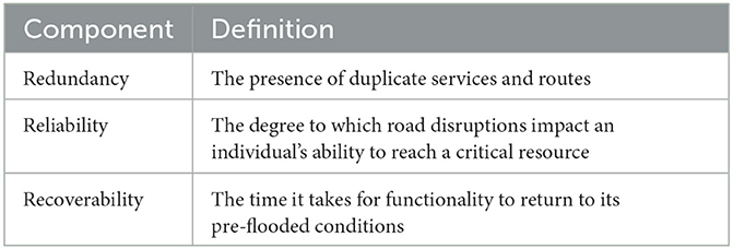
Table 1. Definitions of the components of resiliency: redundancy, reliability, and recoverability.

3. Case-study background and data sources

3.1. Study area

Our study area is Austin, Texas, which is considered one of the fastest-growing cities in the USA, having recently surpassed a total population of 1 million people within the city and 2 million within the metropolitan area. Austin is geographically split by the Colorado River, which runs from west to east through the city. We specifically focus on the formally defined neighborhood boundary of Austin that is north of the Colorado River as it contains the majority of new developments, major creeks, main downtown areas, and population groups within Austin (Figure 1). Our study area is approximately 250-km² and has a population of 300,000. Concurrently with rapid urbanization, Austin is seeing an increase in the occurrence of 1% annual exceedance probability storms, having experienced three in a 5-year window (2013 Halloween Day flood, 2015 Memorial Day flood, and the 2018 Hill Country flood). We use the 2015 Memorial Day flood (25 May 2015) in our analysis, as locals refer to this as being the worst flood in recent Austin history. In 2015, Texas saw intense rainfall events from April through May, causing state and local emergency response agencies to be active throughout the entire month of May and the majority of June (Schumann et al., 2016). On Memorial Day, starting at 19:00 Coordinated Universal Time (UTC), it began to rain in Austin, TX, resulting in 5.2 in. (13.2 cm) of cumulative precipitation in the succeeding 5 h. This value is the second-highest amount of precipitation in a single day in Austin, Texas since 2002 and the eighth-highest amount since 1927, which is the farthest back that uninterrupted records for this region extend. All stream reaches in this study area had their peak instantaneous flow rates around 22:00 UTC.

FIGURE 1

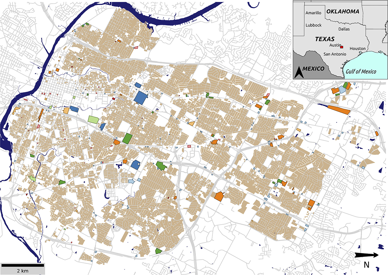
Figure 1. Austin, Texas study area. Residential parcels are shown in tan and critical resource parcels are colored.

3.2. Critical resources and data sources

We leveraged OpenStreetMap data using the open-source Python tools OSMnx (Boeing, 2017) and NetworkX (Hagberg et al., 2008) to obtain, handle, and manipulate the location of critical resources and the road network topology. Open source data can occasionally have incorrect and inconsistent information. Furthermore, gaps can be present in the attributes of road information (e.g., speed limit, number of lanes, road classification). While these drawbacks exist, OpenStreetMap has become a pivotal data source within public, private, and research communities due to the amount and geographic extent of the data (Johnson et al., 2022). To address these limitations, special consideration went into ensuring location accuracy and filling gaps in missing data values. We checked critical resource location layers individually for accuracy and they required only minimal corrections. The road network attributes that our model requires include speed, number of lanes, road width, and capacity. Speed and the number of lanes are sometimes reported in OpenStreetMap but not always and to unknown accuracy. However, OpenStreetMap does have a consistent classification scheme of all of its roadways, and the geographic centerlines are predominantly accurate upon visual inspection. To reduce the impact of inconsistent data reporting of the required attributes, we implemented a relate table based on common national standards to efficiently fill gaps within the data. Table 2 summarizes the road characteristics we used to fill in missing data within the road network when needed. We assumed everything we extracted from OpenStreetMap was accurate and visually inspected for major errors. The only road characteristic that is completely overwritten is the speed limit. Speed limit is sparsely reported in OpenStreetMap and we determined it was more accurate to relate to a completely standardized set of speed limits. Parcel information is not currently available in OpenStreetMap and we therefore acquired it from the Texas Natural Resources Information System. Parcel data are available for the majority of counties/states in the US for free from local government agencies and are typically updated annually.

TABLE 2

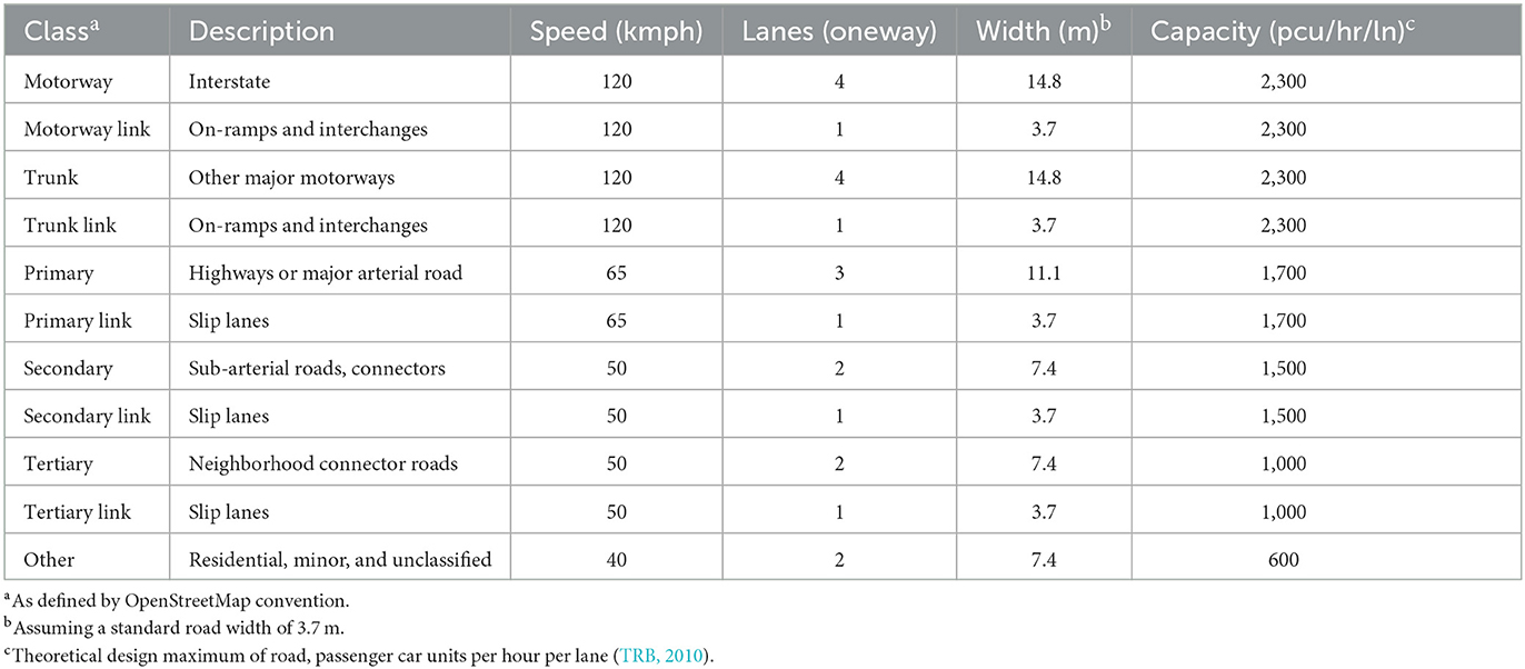
Table 2. Road link classifications and their associated parameters.

Our final network contained 14,057 nodes, 36,027 edges, and 49,612 residential parcels. We identified eight critical resources to examine including grocery stores (37 locations), hospitals (5), pharmacies (25), fire stations (20), police stations (6), emergency medical service stations (11), gas stations (112), and convenience stores (78). We assume residential parcels that share a node with a critical resource to be within walking distance while all others must traverse the road network to access that resource.

4. Methodology

4.1. Inundation and social vulnerability data

We utilized a near-real-time inland compound (fluvial and pluvial) inundation estimate of the Memorial Day flood from previous research and we refer the reader to Preisser et al. (2022) for more information on the methods and results. To summarize, we used outputs from NOAA's National Water Model to map fluvial inundation using GeoFlood (Zheng et al., 2018), an implementation of the HAND method (Nobre et al., 2011) utilizing lidar scale topographic data, and pluvial inundation using Fill-Spill-Merge (Barnes et al., 2021), a topographic depression routing algorithm. The inundation layers used in this study all have a spatial resolution of 1-meter.

We calculate social vulnerability using a factor analysis approach on 27 variables from the U.S. Census Bureau's American Community Survey 5-Year Estimates from 2011–2015 at the block group boundary (Bixler et al., 2021; Preisser et al., 2022). Our SVI calculation is an adapted methodology first developed by Cutter et al. (2003), which utilizes a principal component analysis to similarly reduce the dimensionality of input sociodemographic variables (Supplementary Section 1). Along with the SVI (Figure 2A), we used the two most influential factors as Social Status (Figure 2B) and Economic Status (Figure 2C) indicators to highlight how more specific indicators may capture more inequality compared to generalized indices. The Social Status factor's main contributing Census variables are the people per unit and the percentages of the population that identify as Hispanic, have less than a high school equivalent education, have no health insurance, speak english as a second language, work in extractive/construction industries, are below the poverty line, and are a female headed household. The Economic Status factor's main contributing Census variables are per capita income, median housing value, and the percentage of the households that makes over $250,000 annually.

FIGURE 2

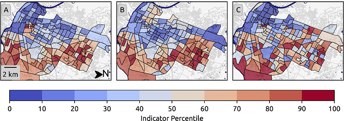
Figure 2. Austin, Texas social vulnerability index, social status (SS), and economic status (ES) indicators at the Census block group boundary using the 2015 American Community Survey 5-Year Estimates. SVI (A) is a factor analysis of relevant sociodemographic variables. SS (B) and ES (C) are the first and second most prevalent factors from the factor analysis.

4.2. Mathematical formulation

The user equilibrium optimization problem (Equation 1), which states that all used routes between each origin and destination pair have an equal and minimal travel time, is subject to three constraints: flow conservation, where link flow must equal path flow (Equation 2), no vehicles left behind, where all flow that goes into a node must exit that node (Equation 3), and no negative flows, where a link cannot have a negative number of travelers (Equation 4). t_ij(x_ij) refers to link performance function (Equation 5), x_ij is a link's flow on link (i, j) in the set of links, A, r and s are the origins and destinations that exist in the set of all nodes, Z, h^π is the number of travelers on path π from (r, s) on the set of all origin destination pairs Π, $δ_{i j}^{π}$ is the number of times path π uses link (i, j), and d^rs is the sum of the number of travelers on every path (r, s).

\begin{array}{l} min_{x, h} & \sum_{(i, j) \in A} \int_{(i, j) \in A}^{x_{i j}} t_{i j} (x_{i j}) d x & (1) \end{array}

\begin{array}{l} s.t. & x_{i j} = \sum_{π \in Π} h^{π} δ_{i j}^{π} \forall (i, j) \in A & (2) \end{array}

\begin{array}{l} d^{r s} = \sum_{π \in Π^{r s}} h^{π} \forall (r, s) \in Z^{2} & (3) \end{array}

\begin{array}{l} h^{π} \geq 0 \forall π \in Π & (4) \end{array}

The link performance function, t_ij(x_ij), or more specifically the BPR function (Equation 5), shows the relationship between a link's travel time, t_ij, the link's traffic flow rate, x_ij, and the links functional or practical capacity, u_ij. The shaping parameters, α and β, determine the rate at which congestion impacts travel times and are often set to 0.15 and 4 respectively. As the flow rate approaches 0, the travel time across the link approaches the congestion free travel time, $t_{i j}^{0}$ . Under normal operating conditions, the congestion free travel time is equal to the speed limit of the link multiplied by the length of the link. We rely on the original BPR function due to its minimal input requirements and simple mathematical form compared to alternative equations (Davidson, 1966; Spiess, 1990; Akçelik, 1991; Mtoi and Moses, 2014). When impacted by ponded water, the speed limit is reduced to the maximum safe driving speed, v(w) (Equation 6). The newly calculated speed limit is multiplied by the link's length to determine the maximum safe congestion free travel time.

\begin{array}{l} t_{i j} (x_{i j}) = t_{i j}^{0} (1 + α {(\frac{x_{i j}}{u_{i j}})}^{β}) & (5) \end{array}

The maximum safe driving speed on a link (km/hr) is a function of the known flood depth on that link, w (mm) (Equation 6). Speed is reduced to 0 km/hr, allowing no vehicular travel, at depths greater than 150 mm (Pregnolato et al., 2017). We utilize the more aggressive standard and its related depth-disruption equation for this study to account for the worst case scenarios (Pregnolato et al., 2017; Arrighi et al., 2019; Tsang and Scott, 2020).

\begin{array}{l} v (w) = 0.003864 w^{2} - 1.1592 w + 86.94 & (6) \end{array}

4.3. Solution methodology

The broad framework for solving all traffic assignment problems can be simplified into four steps. First, given a network with known edge costs, determine the fastest path for each OD pair. Next, based on the previously determined flow paths, recalculate the cost on each edge using the link performance function. With the new edge costs, shift travelers from slower paths to faster paths. Finally, return to the initial step until equilibrium is met and all travelers are on their fastest path. With multiple algorithms available to solve the user equilibrium optimization problem, we chose to use a gradient projection, or path-based, algorithm for its faster convergence speeds (Jayakrishnan et al., 1994). Path-based algorithms break a network down into a list of the utilized paths connecting OD pairs to more efficiently shift travelers between slower and faster routes compared to older link-based algorithms (Frank and Wolfe, 1956).

4.4. Termination criteria

Due to the nature of convex optimization, an exact solution may not be easily calculated and we therefore need a termination criteria to identify when our solution is “good enough” to be considered at equilibrium. To do this, we define the two system states: Total System Travel Time (TSTT) and Shortest Path Travel Time (SPTT). TSTT is the total cost across the network using the estimated traffic assignment, x_ij (Equation 7). SPTT is the cost across the network if all travelers were assigned to the shortest paths, $x_{i j}^{*}$ , based on the previously calculated link costs t_ij(x_ij) (Equation 8). SPTT can also be defined as the sum of the number of travelers between each origin-destination pair, d^rs, multiplied by the shortest path travel time between the origin-destination pair, κ^rs.

\begin{array}{l} T S T T = \sum_{(i, j) \in A} t_{i j} (x_{i j}) x_{i j} & (7) \end{array}

\begin{array}{l} S P T T = \sum_{(i, j) \in A} t_{i j} (x_{i j}) x_{i j}^{*} = \sum_{(r, s) \in Z^{2}} κ^{r s} d^{r s} & (8) \end{array}

To determine when a solution is close enough, we calculate the Average Excess Cost, or AEC (Bar-Gera, 2002). The AEC represents the average difference between the travel time on each traveler's actual path and the travel time on the shortest path available to them, having units of time (Equation 9). We consider convergence when the AEC is less than or equal to 0.01 seconds. An exact solution to the traffic assignment problem is found when TSTT is equal to SPTT, otherwise TSTT will always be larger.

\begin{array}{l} A E C = \frac{\sum_{(i, j) \in A} t_{i j} (x_{i j}) x_{i j} - \sum_{(r, s) \in Z^{2}} κ^{r s} d^{r s}}{\sum_{r s \in Z^{2}} d^{r s}} = \frac{T S T T - S P T T}{\sum_{r s \in Z^{2}} d^{r s}} & (9) \end{array}

4.5. Calculating resiliency metrics

We chose to adapt the resiliency definition matrix from Lim et al. (2022) because of their emphasis on measuring and defining resiliency at multiple scales. The goal of analyzing these components at the network at individual scales is to: (1) provide insight on network performance characteristics that can better inform city and regional response efforts and (2) describe high-resolution household impacts that complement high-resolution inundation estimates. Based on the resiliency component definitions (Table 1), we create a metric for each component at the network and individual scale (Table 3). We aggregate each metric to the underlying Census block group in order to compare them with an SVI and other relevant sociodemographic indicators.

TABLE 3

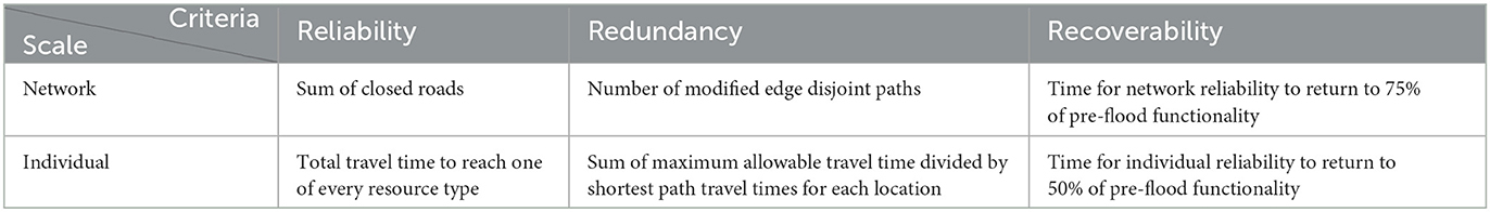
Table 3. Description of individual and network scale metrics, summed within each Census block group to compare against sociodemographic data.

4.5.1. Redundancy

We calculate network redundancy scores using a modified edge disjoint paths. A node's edge disjoint paths value is the number of alternative routes that exist between that node and a specified destination that have no overlapping edges. Because of the sparse nature of road networks, it often only takes the removal of one or two edges to disconnect an origin to a destination (e.g., a house that lives on a residential road only has two directions to travel). Therefore, we use a neighbors-of-neighbors approach and calculate the total number of disjoint paths from all of the neighbors of the neighbors (i.e., two network links away neighbors) of the origin and destination (Lhomme et al., 2013). Household redundancy scores are equal to the sum of OD travel times for each household to reach each location of each resource divided by a maximum allowable travel time (15-min), if the travel time is less than the maximum allowable travel time. For both redundancy scores, a higher value represents a more redundant connection for an origin and that resource.

4.5.2. Reliability

Network reliability scores are the total number of closed roads within each block group. Household reliability scores are the sum of the total travel time for a household to travel to the nearest available option for each resource type. We give unreachable resources a representatively large travel time to represent the cost of not being able to access that resource. For this study, we set that value to 4 times the maximum travel time across the study area to access that resource.

4.5.3. Recoverability

Network and household recoverability metrics are the time it takes the reliability metrics to return to 75 and 50% respectively, of their pre-flood condition values. We chose these threshold percentages due to a large number of block groups being considered recovered at these values. Different threshold percentages produce nearly the same recoverability Lorenz curves since these plots measure the relative distribution of burdens and the trajectory of the number of block groups that are considered recovered using various thresholds are all nearly identical (Supplementary Section 2).

4.6. Measuring equality and equity with resiliency metrics

We calculated resiliency metrics using hourly inundation estimates between 18:00 UTC (25 May 2015) and 17:00 UTC (26 May 2015). Rainfall began to fall around 19:00 UTC, and therefore the network before this time is at pre-flood conditions. Peak-flood conditions (i.e., largest compound inundation extent) occur at 22:00 UTC, which coincides with the estimated peak number of road closures (Figure 3). To determine each metric at each time step, we overlay the road network with the inundation estimate (Figure 4A), run the traffic assignment algorithm (Figure 4B), and calculate the resultant network redundancy (Figure 4C), network reliability (Figure 4D), household redundancy (Figure 4E), and household reliability (Figure 4F) metrics.

FIGURE 3

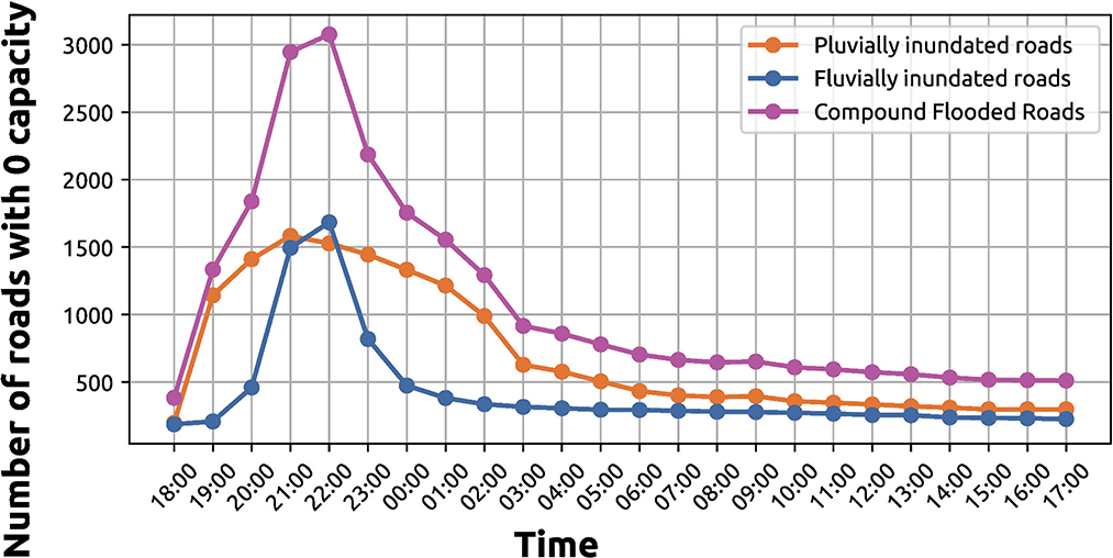
Figure 3. Austin, Texas time series of total modeled closed roads caused from fluvial, pluvial, and compound flooding. A road is considered closed and impassable if it has over 15-cm of ponded water.

FIGURE 4

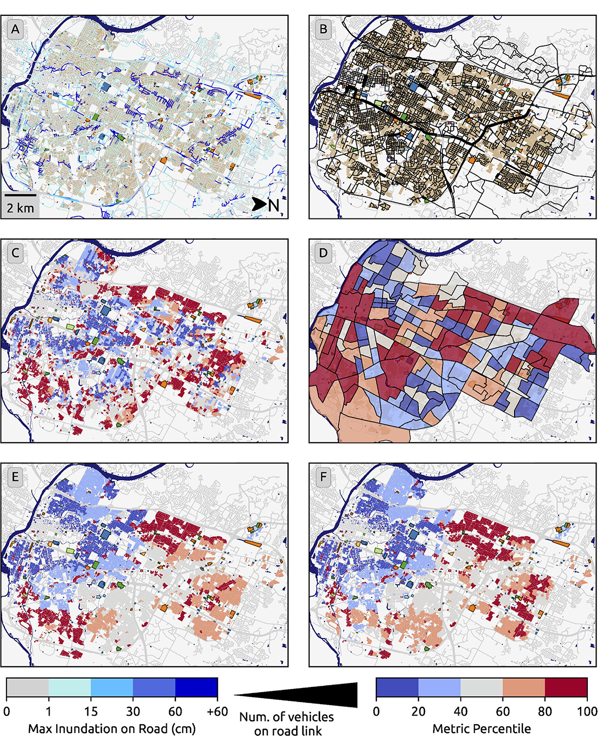
Figure 4. Austin, Texas inundated road network (A) and the resultant traffic assignment solution (B) at peak flood conditions during the Memorial Day flood (22:00 25 May 2015). Network redundancy (C), network reliability (D), household redundancy (E), and household reliability (F) show the spatial distribution of metric values across the study area at peak flood conditions.

In order to quantify equality, we use Lorenz curves and calculate the associated Gini coefficients, which were originally developed to measure income inequality (Morgan, 1962). A typical Lorenz curve plots the percentile ranking of households' net worth on the x-axis and the percentage of cumulative income on the y-axis. In a perfectly equitable society, the Lorenz curve would match a 1:1 line. The Gini coefficient is a measure of deviation from the perfectly equitable society (Gini = 0), where a value of –1 and 1 are perfect inequity, favoring the bottom and top net worth of households respectively. Lorenz curves are gaining a renewed interest in measuring inequality and have recently been applied to other flood risk studies (Sanders et al., 2022; Yarveysi et al., 2023). For this application, the x-axis of the Lorenz curve is the social vulnerability (or social/economic status) index percentile and the y-axis is the specific variable being measured for each metric. To maintain similarity between Lorenz curves for ease of readability, we normalize (0–1) all y-axis variables and reflect necessary variables to ensure that a Gini coefficient greater than 0 represents inequality benefiting the least vulnerable. Furthermore, we weight each y-axis variable by the people per unit Census variable (i.e., average number of people living in a house) to account for population density discrepancies. We also calculate the quartile burden, which is equal to the normalized cumulative sum of the metric under investigation for that percentile of the population with Q1 representing the least vulnerable and Q4 the most vulnerable quarter of the population.

It is important to note that by itself, Lorenz curves and Gini coefficients measure equality because they examine the distribution of a variable across a population. However, in response to a flood event, equity may be a more substantive measure because communities feel the impacts of flood events differently. For example, if two households experience the same amount of flooding, but one is more vulnerable due to an underlying condition (e.g., is food insecure, has to go to a hospital for treatment regularly, lives in an area susceptible to crime, etc.), then the impacts of the flood are not felt equally. Therefore, we also present the same resiliency metrics weighted by the SVI, social status, and economic status indices to highlight the existence of flood impact inequities. It is not clearly defined the exact degree to which sociodemographic vulnerability affects an individual. To account for this uncertainty in determining hazard impact equity, we use multiple weighting schemes based on a range of potential thresholds. Equation 10 produces a weighting factor for each metric. We calculated each block group's weight by first determining its indicator (SVI, SS, or ES) rank, with the least vulnerable block group having a rank of 0 and the most vulnerable block group having a rank equal to the number of observations (n_obs). p is the percentage weight, or the degree to which an individual's sociodemographic vulnerability influences their ability to respond. The least vulnerable block group's weight is equal to 1 − p, while the most vulnerable block group's weight is equal to 1 + p, and every block group in between has a weight value equally spaced between the minimum and maximum.

\begin{array}{l} w e i g h t = (1 - p) + \frac{(r a n k) (2 * p)}{n_{o b s}} & (10) \end{array}

5. Results

We present network resiliency results while considering different flood sources (fluvial, pluvial, and compound) to address how regulators might have to respond differently based on the prevailing flood type. Additionally, we present individual resiliency results while considering the holistic SVI as well as the Economic Status (ES) and Social Status (SS) indicators, to draw attention to different measures of socio-demographic variables.

5.1. Network scale

5.1.1. Redundancy

Our estimated network redundancy at peak-flood conditions shows a slightly unequal distribution when only considering pluvial flooding (G = 0.09), a near equal distribution when only considering fluvial flooding (G = –0.01), and compound flooding in between the two (G = 0.03) (Figure 5). Q2 (the second least vulnerable quarter of the population) and Q4 (the most vulnerable quarter of population) carry the most network redundancy burden across all of the flood source scenarios. The gap in network redundancy between the quarters of the population that carry the most and least burden is 15, 12, and 14 percentage points for compound, fluvial, and pluvial flooding respectively.

FIGURE 5

Figure 5. Austin, Texas network redundancy Lorenz curve at peak-flood conditions during the Memorial Day flood (22:00 25 May 2015). Block group network redundancy is weighted by the population per housing unit (i.e., density) and normalized from 0 to 1.

FIGURE 6

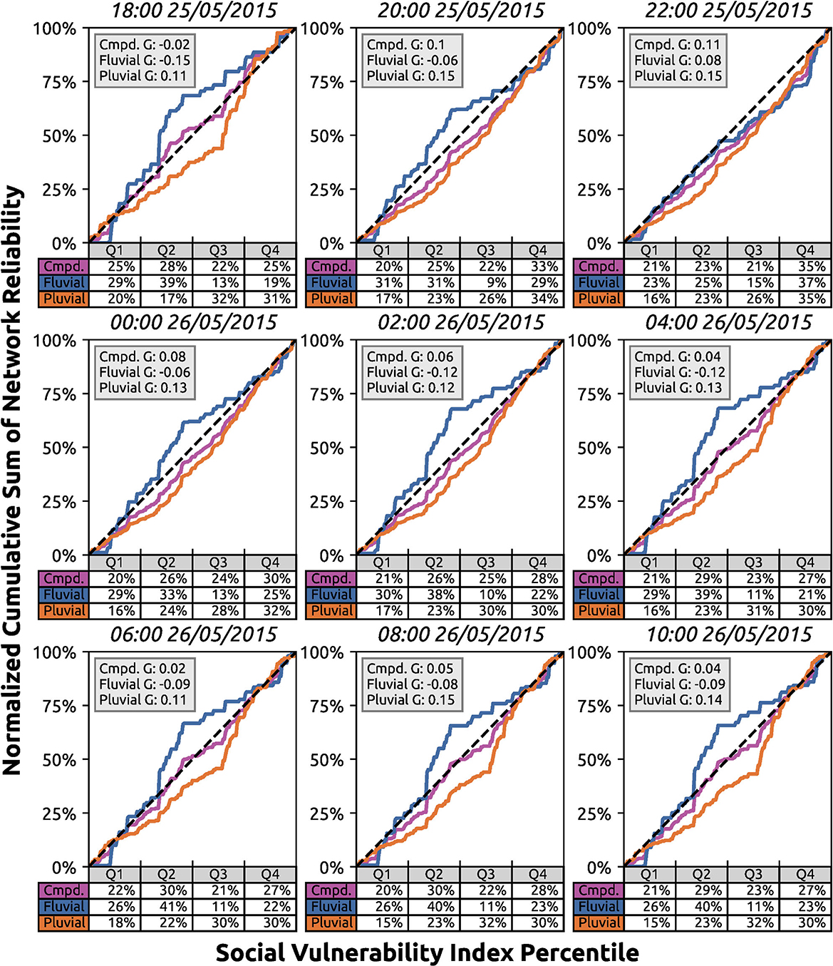
Figure 6. Austin, Texas network reliability during the Memorial Day flood (25 May 2015) and shown here in 4-h increments. Network reliability is calculated every hour and shown in 4-h increments for brevity. Block group network reliability is weighted by the population per housing unit (i.e., density) and normalized from 0 to 1.

While we calculated network redundancy for each time step, there was little to no change from one observation to the next. This result suggests that either this particular storm does not have a significant impact on the number of available routes for households to access resources, or that the storm is maintaining an equal impact across the study area. The latter is less likely as the subsequent results show more substantial unequal impacts over time. The former is more likely because urban areas are typically characterized by highly connected road networks, suggesting that network route redundancy is not the reason for resource accessibility discrepancies (Supplementary Section 3).

5.1.2. Reliability

Before rainfall begins (18:00), the network reliability burden lies on the least vulnerable half of the population for fluvial flooding (G = –0.15), but lies on the more vulnerable half of the population for pluvial flooding (G = 0.11). This pre-rainfall inequality can be attributed to the base conditions that the study area is experiencing as a result of days of saturated conditions prior to the event of interest. The compound flooding network reliability burden is therefore in between the two, and appears to be more equally distributed (G = –0.02). A shift occurs at peak flood conditions (22:00) and Q4 carries the highest network reliability burden for compound (35%), fluvial (37%), and pluvial (35%) flooding. The Gini coefficients for compound, fluvial, and pluvial flooding all increase by 0.13, 0.23, and 0.04 respectively. Pluvial flooding always impacts the more vulnerable half of the population throughout the duration of the flood event, with the Gini coefficient remaining above 0.11. Post-peak-flood, the burden of fluvial flooding returns to the least vulnerable half of the population, predominantly on Q2 (33–41% of the burden depending on time), suggesting that fluvial flooding in these block groups is more persistent and recedes at a slower rate compared to other block groups. Due to the near opposite impacts of fluvial and pluvial flooding, compound flooding has a more equally distributed impact, with a Gini coefficient of less than 0.06 at all times except for the 2 h pre- and post-peak-flood. While the compounding events of a flood may result in a more equal distribution of impacts, the underlying flood sources distinctly impact population groups differently.

5.1.3. Recoverability

Network recoverability shows the most unequal distribution when compared against pluvial flooding (G = 0.12), closer to equal for fluvial flooding (G = 0.06), and in between for compound flooding (G = 0.1) (Figure 7). Q4 carries the greatest network recoverability for compound (30%), fluvial (31%), and pluvial (31%) flooding, with Q3 carrying a similarly high burden for compound (29%) and pluvial flooding (29%). Q2 carries the second highest fluvial burden (30%). The high burdens associated with Q4 pluvial flooding and Q2 fluvial flooding coincide with the network redundancy and reliability behaviors.

FIGURE 7

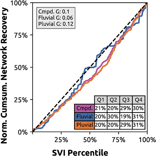
Figure 7. Austin, Texas network recoverability during the Memorial Day flood (25 May 2015). Block group network recoverability is weighted by the population per housing unit (i.e., density) and normalized from 0 to 1.

5.2. Household scale

5.2.1. Redundancy

Household redundancy at pre-flood conditions is near perfect equality when compared against SVI (G = –0.02), and is further unequal for ES (G = –0.04) and SS (G = –0.14) (Figure 8). Additionally, Q1 carries the highest household redundancy burden when compared against SVI (27%), SS (30%), and ES (30%). Negative G values further show that the least vulnerable portion of the population carries the higher burden during pre-flood conditions. However, Gini coefficients and burdens shift across all indices to the most vulnerable half of the population at peak flood conditions. SVI, SS, and ES Gini coefficients all increase by more than 0.30 when comparing pre-peak to peak-flood conditions. Additionally, the Q4 SVI, SS, and ES burdens all nearly double during this time, while Q1 goes from carrying the most to the least burden.

FIGURE 8

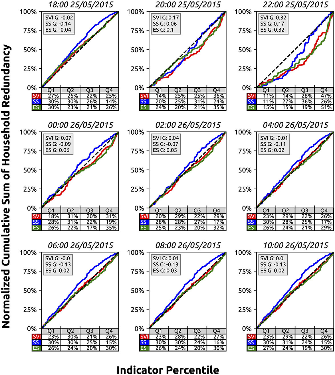
Figure 8. Austin, Texas household redundancy during the Memorial Day flood (25 May 2015) and shown here in 4-h increments. Household redundancy is calculated every hour and shown in 4-h increments for brevity. Block group household redundancy is weighted by the population per housing unit (i.e., density) and normalized from 0 to 1.

5.2.2. Reliability

Household reliability at initial conditions is unequal for SVI (G = 0.1), SS (G = 0.23), and ES (G = 0.11) (Figure 9). Concurrently, Q4 carries the highest burden for SVI (34%), SS (38%), and ES (32%). This inequality is persistent throughout the flood event, with the most vulnerable quarter of the population consistently having to travel further to access critical resources. Burden values return to their near pre-flood conditions within 6 h post-peak flood, with Gini coefficients only having slight fluctuations and burdens staying relatively unchanged.

FIGURE 9

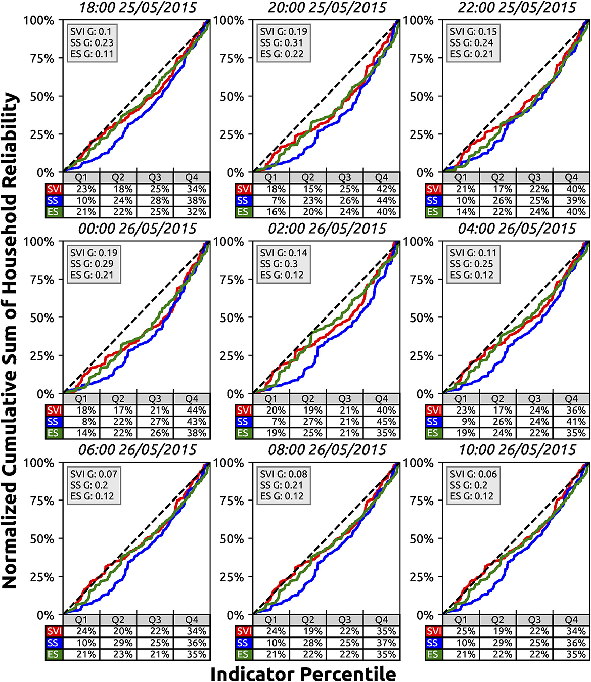
Figure 9. Austin, Texas household reliability during the Memorial Day flood (25 May 2015) and shown here in 4-h increments. Household reliability is calculated every hour and shown in 4-h increments for brevity. Block group household reliability is weighted by the population per housing unit (i.e., density) and normalized from 0 to 1.

Q1 and Q3 household reliability burdens strictly decrease when comparing conditions between the pre-flood values to 6 h post-peak, while Q2 burdens experience a mixture of slightly increasing and decreasing values. Q4 burdens only increase during this time, showing that throughout the flood event burden is predominantly transferred to the most vulnerable quarter of the population. This result suggests the Q4 household reliability is more susceptible to changes compared to other parts of the population. In conjunction with this, Q1 household reliability burdens across indices never increase from the pre-flood conditions, with the one exception of SVI which increases by only 1–2 percentage points 10–12 h after peak-flood. Over the entire flood event, SVI and ES are relatively similar in terms of Gini coefficients and the distribution of burdens. On the contrary, SS has a Gini coefficient that is between two and three times as large, which can be attributed to the minimal burden that Q1 carries which never exceeds 10%. This result highlights how different vulnerability and socioeconomic indicators show different levels of inequality based on what they specifically measure.

5.2.3. Recoverability

Household recoverability continues to show the same trends, with burdens being distributed unequally when compared against SVI (G = 0.11), SS (G = 0.16), and ES (G = 0.12) (Figure 10). Q4 and Q1 carry the highest and lowest household recoverability burdens respectively.

FIGURE 10

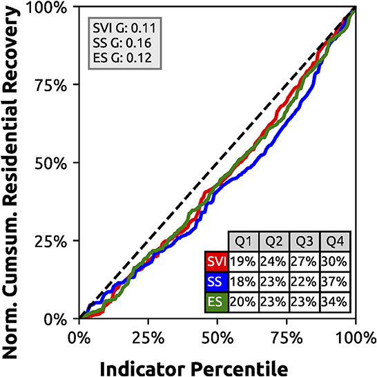
Figure 10. Austin, Texas household recoverability during the Memorial Day flood (25 May 2015). Block group household recoverability is weighted by the population per housing unit (i.e., density) and normalized from 0 to 1.

5.3. Household equity

We calculate household equity at peak flood conditions using percentage weights of 25, 50, and 100% (Figure 11). As expected, each metric becomes more unequally distributed as the percentage weight increases. Q4 burdens approach 50–60% for the majority of scenarios across indices, metrics, and percentage weights. At the same time, Q1 burdens are predominantly near or below 10%. The average difference in burden that Q4 carries over Q1 across indices, metrics, and percentage weights is equal to 41 percentage points.

FIGURE 11

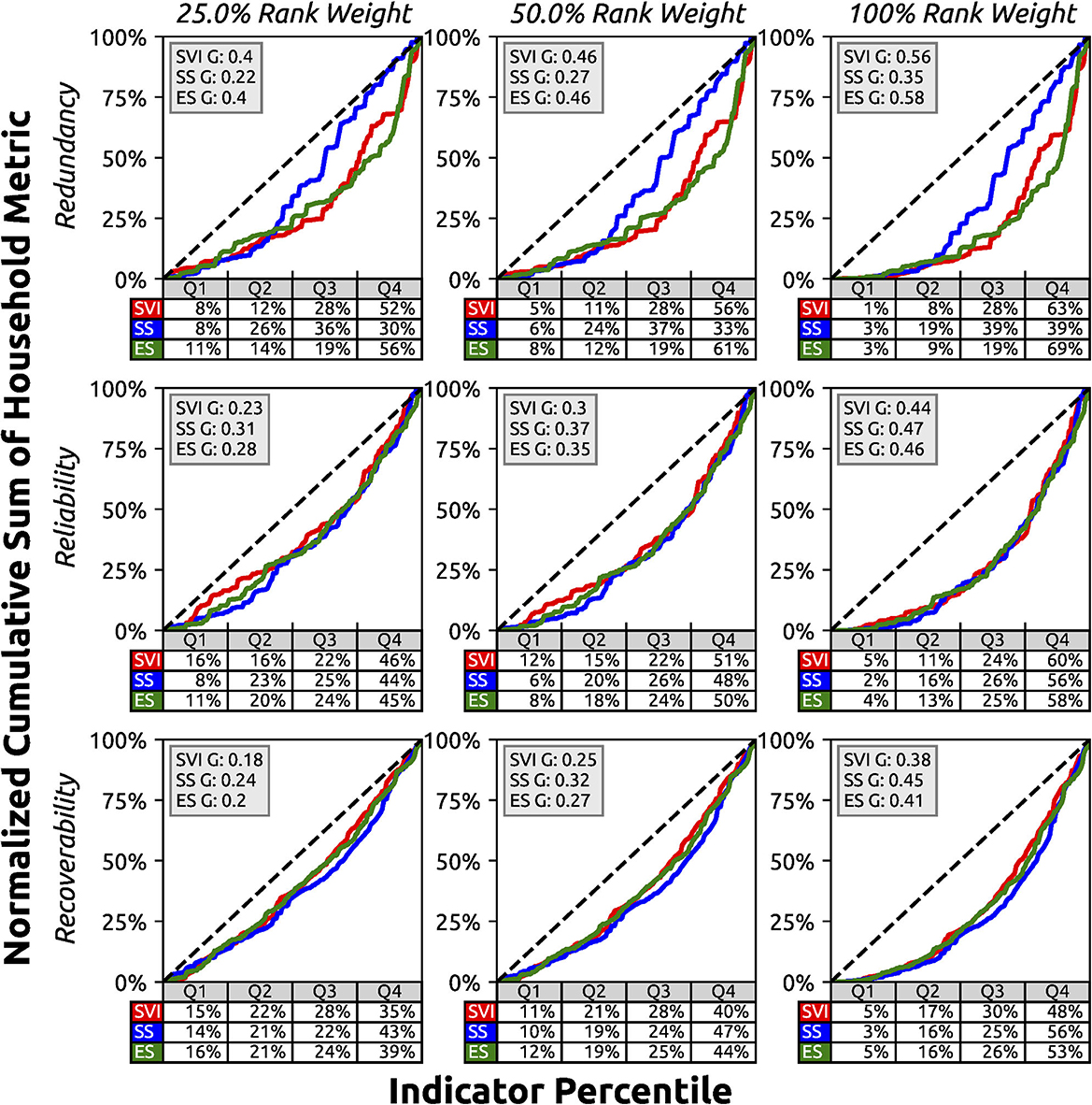
Figure 11. Austin, Texas household redundancy, reliability, and recoverability metrics during the Memorial Day flood at peak flood conditions (22:00 25 May 2015) while under the influence of 25, 50, or 100% indicator rank weight. Rank weights are the degree to which equality Lorenz curves are weighted by the block group indicator ranks.

6. Discussion

6.1. Disproportional distribution of burdens across scales, flood types, and indicators

Every metric shows a disproportional distribution of the effects of flooding on an individual's ability to access critical resources. At peak flood conditions, Q4 carries the highest burden regardless of flood type and vulnerability indicator (Figures 5–10). The only exceptions are network redundancy under the influences of compound and fluvial flooding (second highest burden) and household redundancy when compared against social status (most volatile, burden doubles when compared to pre-flood conditions). Concurrently, Q1 regularly carries the lowest burden during peak-flood conditions. At the network scale, Q1 consistently carries the smallest burden for pluvial and compound flooding, and the second lowest for fluvial. At the household scale, Q1 carries two to four times less burden when compared to Q4 across all vulnerability indicators.

Network metrics highlight the duality of fluvial and pluvial flooding (Figures 5–7). While fluvial flooding typically impacts the least vulnerable half of the population, pluvial flooding typically impacts the most vulnerable half of the population. Therefore, compound flooding appears to be relatively more equally distributed. While the numbers of roads closed by pluvial and fluvial flooding at peak-flood conditions are within 5% of each other (Figure 3), there are higher magnitude inequalities across all household metrics (Figures 8–10). This result suggests that while compound flooding may appear to affect the network equally, its impacts at the household level are not, further justifying the need to analyze hazard events at multiple scales simultaneously.

Household metrics are complementary to each other, showing a disproportionate burden distribution regardless of the vulnerability indicator (Figures 8–10). Social status shows the most disproportionality because it has the highest Gini coefficients with respect to household reliability and recoverability and is the most volatile with respect to household redundancy. The observable volatility in household redundancy and network reliability is likely a factor of the large number and the subsequent decrease of flooded roads caused by fluvial flooding at and immediately after peak-flood conditions (Figure 3). Therefore, more persistent flooding from pluvial sources is what likely causes the longer lasting inequality issues. Across the event we observe metrics returning close to their pre-flood conditions 6 h after peak-flood occurs. While this was a relatively short storm event, it is necessary to understand persistent pluvial flooding's role in affecting communities immediately after a flood event. While the majority of roads have reopened within 18-h post-peak flood conditions, Lorenz curves and Gini coefficients only show relative disproportionality and burdens. For this specific storm, there is still ponded water persisting along roadways and while not deep enough to close roads, will still influence travel time. Remaining ponded water along roadways is another source of inequity as longer travel times to critical resources can be the difference in life and death (e.g., longer travel times to hospitals can be a serious threat and is not just an inconvenience) (Ingenfeld et al., 2018; Clark et al., 2022).

6.2. The most vulnerable are the least resilient

Despite a large portion of flood risk communication studies existing only in the context of theoretical frameworks (Kellens et al., 2012), researchers have identified that stakeholders need flood dynamics information (where and when floods will occur) in order to make informed decisions (Rollason et al., 2018) and are willing to accept a higher degree of uncertainty in order to receive more timely information (McCarthy et al., 2007). The misalignment between recent advancements in flood inundation research and these needs has led to the slower adoption of knowledge by flood management stakeholders, generating a push across disciplines to move beyond the “hot spots and hot moments” framework to better understand the temporal and spatial characteristics of events as they develop, occur, and unfold (Bernhardt et al., 2017; Coles et al., 2017). Additionally, there are established needs for flood impact models to consider transportation infrastructure disruptions (Yarveysi et al., 2023), as well as for models with high speeds and flexibility in order for multiple stakeholders to adopt new methods in existing flood risk management systems (Leskens et al., 2014).

Our high temporal and spatial analysis of resource accessibility shows that the most vulnerable quarter of the population are the least resilient to the effects of a flood. For example, Q4 household redundancy burdens double during peak flood conditions, while Q1 burdens are halved (Figure 8). Similarly at the network level, a temporal analysis captures the shifting nature of burdens, with Gini coefficients increasing and decreasing rapidly around peak-flood conditions, highlighting the necessity to analyze the temporal consequences of a flood event (Figure 6). Furthermore, by identifying the specific quarters of the population that are most vulnerable, we are better able to capture discrepancies amongst the total population. One specific example of this is the household reliability metric when compared against social status at 0:00 26/06/2015 (Figure 9). If we only examined halves of the population, we would witness the most vulnerable half carrying just over twice as much burden. However, comparing Q4 to Q1 we see that the most vulnerable quarter carries over five times as much burden compared the least vulnerable quarter. These more targeted results can better allow emergency managers to respond with greater efficiency and precision.

Equality is not necessarily the goal when determining the impact of a natural hazard. For example, a hazard could affect every individual equally (G = 0), but this would be a less desirable solution than if only a handful of individuals were impacted (G ≠ 0) (Logan et al., 2021). While a Gini coefficient between 0.3-0.4 is typically considered a reasonable gap when strictly using income data, evidence suggests that the threshold is less when examining inequalities in flood risk and vulnerability (Sanders et al., 2022; Yarveysi et al., 2023). Our peak Gini coefficients for household redundancy (SVI at peak flooding, G = 0.32, Q4 = 47%) and household reliability (SS 4 h post peak flooding, G = 0.30, Q4 = 45%) are two examples representing steep disproportionalities in the distribution of impacts. While the Gini coefficient is a valuable tool to quickly identify inequality, it is still necessary to account for the magnitude of impacts and the disproportionate effects of that burden to understand how to respond equitably (Osberg, 2016).

When we factor in the degree to which being vulnerable to floods reduces an individual's ability to cope with its effects, the disproportionality only increases (Figure 11). While researchers have identified the inequitable impacts of flooding and other environmental disasters (Cutter et al., 2003; Chakraborty et al., 2019; Moulds et al., 2021; Wing et al., 2022), the exact combination of what sociodemographic variables that make an individual more at risk and to what degree (i.e., the equity rank weight) are highly variable. A moderate influence of 25% (Toland et al., 2023) exacerbates burdens such that Q4 carries on average 4 times as much burden as Q1. By analyzing multiple vulnerability indicators with multiple rank weights, we can draw attention to the social status variables that are more disparate in Austin during this particular hazard event which can aid in further storm management planning.

The exclusion of pluvial flooding from most emergency flood mapping sources is another source of inequality/inequity (Grahn and Nyberg, 2017). Pluvial flooding specifically leads to ponded water on impervious surfaces, such as roadways and intersections, that would otherwise not be identified as being inundated using common flood risk maps (Preisser et al., 2022). Our results show that pluvial flooding doubles the number of closed roads at peak flood conditions and predominantly impacts more vulnerable communities. If we utilized inundation maps that only included fluvial flooding, our network and household metrics would drastically underrepresent the disproportional distribution of burdens, perpetuating unequal and inequitable flood risk exposures.

6.3. Applicability for improving disaster preparedness and future work

The model we have developed is solely built on open-source data, which fall into three main categories: infrastructure (road and resource locations), inundation, and socioeconomic data. Infrastructure data retrieved from OpenStreetMap are already available for a large portion of the world (Barrington-Leigh and Millard-Ball, 2017). While there are certainly gaps in data availability in some nations and rural areas, OpenStreetMap continues to expand its global reach. There will always be issues with accuracy with crowdsourced road network and resource data, but strict data quality policies continue to raise the reliability and usability of OpenStreetMap data. Resource location data are also easily verifiable for each study location and require minimal levels of local knowledge.

Our framework can accept any inundation layer or road closure information to estimate network disruptions. Users can opt to use existing inundation estimates that they have available. Our specific pluvial and fluvial inundation layers are reproducible anywhere mid- or high- resolution digital elevation models exist. Lower resolution elevation data (30-meters) can also be used, with the understanding that modeling urban flooding with such data comes with its own uncertainties and weaknesses. Our inundation layers are created using the open source tools GeoFlood (Zheng et al., 2018) and Fill-Spill-Merge (Barnes et al., 2021) that estimate fluvial and pluvial flooding respectively (Preisser et al., 2022). This process can be replicated anywhere in the United States using data from NOAA's National Water Model (NWM), which contains the necessary stream flow and ponded water data going back to the 1980s to produce the relevant inundation estimates. These tools can also be run without NWM data and only require estimated/observed runoff depths and stream flow values and can therefore be applied across the globe.

Socioeconomic data from the 5-Year American Community Survey are already available for the entire United States from 2009–2021 and will continue to be released in the foreseeable future. While socioeconomic data may be less accessible in other parts of the world, similar layers of vulnerability are still commonly produced by other nations. While the Gini coefficients and Lorenz curves would not be possible without underlying vulnerability information, our model will still quantify household and neighborhood resource accessibility disparities. Despite the unknown degree to which sociodemographic variables influence inequities, the resiliency metrics we computed highlight inequalities which can directly aid emergency managers in the pre-placement of supplies and personel before a flood event occurs. Communities across the United States are employing resource hubs, or “resiliency hubs,” as a way to better prepare for disasters (Anderson et al., 2017). While studying the performance of infrastructure networks during disasters is not new (Kameshwar et al., 2019), there has been limited use of transportation planning in resiliency hub placement and design (Ciriaco and Wong, 2022). Furthermore, household metrics can be utilized by individuals in their own emergency planning to gain a more holistic picture of how they may or may not be able to access necessary resources. The application of our framework to community and regional planning can directly provide information about gaps in resource coverage, which can aid in data-driven decision-making processes.

7. Conclusion

We created a model that solves the user equilibrium traffic assignment problem that routes every household to their nearest critical resources while under the influence of a flood event. Our model's capabilities to calculate hourly inundation impact at the household level, utilizing only open-source data and low-computational resources (i.e., without the use of high performance computers or GPUs), is a step towards a more accessible method for measuring the near-real time effects of floods on transportation networks in the context. Our method is capable of discerning the dynamic nature of resource accessibility throughout time that would otherwise go unnoticed when only considering worse-case scenario flood extent maps. Our matrix of metrics creates a holistic picture of individual and network scale results which is able to capture the multiple components of resiliency. In terms of resource accessibility and in the context of our study area Austin, Texas, we identified that the most vulnerable households are the most susceptible to the effects of a flood event, the least vulnerable carry the smallest burden, and that small inequalities can become large inequities when considering the degree to which being more vulnerable impacts one's ability to cope with a hazard.

Data availability statement

All data used in this analysis are publicly available and obtained from their respective sources, including NOAA, USGS, TNRIS, OpenStreetMap, and the U.S. Census Bureau. The GeoFlood and Fill -Spill -Merge codes can be found on their respective GitHub pages (https://github.com/r-barnes/Barnes2020-FillSpillMerge, Barnes, 2022; https://github.com/passaH2O/GeoFlood, Passalacqua, 2010). All associated codes that we used in this study can be retrieved from https://doi.org/10.5281/zenodo.8350297. We refer users to our GitHub page for the most recent versions of our tools https://github.com/mdp0023/network_analysis.

Author contributions

MP: Conceptualization, Data curation, Formal analysis, Investigation, Methodology, Software, Visualization, Writing—original draft, Writing—review and editing. PP: Conceptualization, Formal analysis, Investigation, Supervision, Writing—original draft, Writing—review and editing. RB: Supervision, Writing—review and editing. SB: Supervision, Writing—review and editing.

Funding

The author(s) declare financial support was received for the research, authorship, and/or publication of this article. Funding was provided by the National Science Foundation Graduate Research Fellowship (NSFGRFP, grant no. DGE-1610403), the Future Investigators in NASA Earth and Space Science and Technology (NASA FINESST, grant no. 21-EARTH21-0264), and PlanetTexas2050, a research grand challenge at the University of Texas at Austin.

Acknowledgments

We thank the reviewers and editor for providing valuable comments that have improved the clarity and contents of this paper.

Conflict of interest

The authors declare that the research was conducted in the absence of any commercial or financial relationships that could be construed as a potential conflict of interest.

Publisher's note

All claims expressed in this article are solely those of the authors and do not necessarily represent those of their affiliated organizations, or those of the publisher, the editors and the reviewers. Any product that may be evaluated in this article, or claim that may be made by its manufacturer, is not guaranteed or endorsed by the publisher.

Supplementary material

The Supplementary Material for this article can be found online at: https://www.frontiersin.org/articles/10.3389/frwa.2023.1278205/full#supplementary-material

References

Akçelik, R. (1991). Travel time functions for transport planning purposes: Davidson's function, its time dependent form and alternative travel time function. Austr. Road Res. 21, 49–59.

Google Scholar

Akhavan, A., Phillips, N. E., Du, J., Chen, J., Sadeghinasr, B., and Wang, Q. (2019). Accessibility inequality in houston. IEEE Sens. Lett. 3, 1–4. doi: 10.1109/LSENS.2018.2882806