 Renske J. E. Vroom1*
 Sarian Kosten1Rafael M. Almeida2
 Raquel Mendonça3Ive S. Muzitano3,4Icaro Barbosa3
 Jonas Nasário3
 Ernandes S. Oliveira Junior5Alexander S. Flecker6Nathan Barros5
- 1Department of Aquatic Ecology and Environmental Biology, Radboud Institute for Biological and Environmental Sciences, Radboud University, Nijmegen, Netherlands
- 2School of Earth, Environmental, and Marine Sciences, The University of Texas Rio Grande Valley, Edinburg, TX, United States
- 3Department of Biology, Federal University of Juiz de Fora, Juiz de Fora, Brazil
- 4Fishing Institute Foundation of the State of Rio de Janeiro, Rio de Janeiro, Brazil
- 5Graduate Program of Environmental Sciences, Laboratory of Ichthyology of the North Pantanal, University of the State of Mato Grosso, Cáceres, Brazil
- 6Department of Ecology and Evolutionary Biology, Cornell University, Ithaca, NY, United States
An ever-increasing demand for protein-rich food sources combined with dwindling wild fish stocks has caused the aquaculture sector to boom in the last two decades. Although fishponds are potentially strong emitters of the greenhouse gas methane (CH4), little is known about the magnitude, pathways, and drivers of these emissions. We measured diffusive CH4 emissions at the margin and in the center of 52 freshwater fishponds in Brazil. In a subset of ponds (n = 31) we additionally quantified ebullitive CH4 fluxes and sampled water and sediment for biogeochemical analyses. Sediments (n = 20) were incubated to quantify potential CH4 production. Ebullitive CH4 emissions ranged between 0 and 477 mg m−2 d−1 and contributed substantially (median 85%) to total CH4 emissions, surpassing diffusive emissions in 81% of ponds. Diffusive CH4 emissions were higher in the center (median 11.4 mg CH4 m−2 d−1) than at the margin (median 6.1 mg CH4 m−2 d−1) in 90% of ponds. Sediment CH4 production ranged between 0 and 3.17 mg CH4 g C−1 d−1. We found no relation between sediment CH4 production and in situ emissions. Our findings suggest that dominance of CH4 ebullition over diffusion is widespread across aquaculture ponds. Management practices to minimize the carbon footprint of aquaculture production should focus on reducing sediment accumulation and CH4 ebullition.
1. Introduction
With the current growth in global population and improving living standards, the demand for high-protein food sources is rapidly increasing (Henchion et al., 2017). Fish has historically played an essential role as an animal food source, and is rich in protein, essential fatty acids, and micronutrients (Arts et al., 2001; Kawarazuka, 2010; Hicks et al., 2019). Until the 1990s, nearly all demand for fish was supported by capture fisheries (FAO, 2020). However, wild fish stocks are dwindling rapidly due to overfishing, and capture fishery production has plateaued over the past two decades (FAO, 2020). Accordingly, the increasing demand for fish has been supported by meteoric growth in aquaculture production. Globally, the contribution of aquaculture to total fish production has risen from 26% in 2000 to 46% in 2016–2018 and is expected to increase to 53% by 2030, surpassing capture fisheries production (FAO, 2020). However, this massive increase comes with environmental costs, such as substantial greenhouse gas (GHG) emissions (Kosten et al., 2020).
Most aquaculture production is freshwater based (63% in 2018), and the majority of freshwater aquaculture facilities use earthen ponds, which are shallow, excavated structures consisting solely of soil materials (FAO, 2020). To optimize production, these ponds often receive large amounts of fish feed and fertilizers. This external input of organic matter and nutrients could lead to environmental pollution, including high emissions of the greenhouse gas (GHG) methane (CH4) (Vasanth et al., 2016; Wu et al., 2018; Yuan et al., 2019). CH4 is a strong GHG with a 27 times higher global warming potential than carbon dioxide (CO2) on a 100-year time horizon (Canadell et al., 2021). CH4 production takes place during the breakdown of organic matter, mostly under anoxic conditions. High levels of nutrients, such as nitrogen (N) and phosphorous (P), can exacerbate CH4 emissions by increasing primary production, and, therefore, substrate availability for methanogens (e.g., Whiting and Chanton, 1993; DelSontro et al., 2016; Beaulieu et al., 2019). Fishpond CH4 emissions may be minimized by climate-smart management, enabling sustainable protein production for biodiversity and the climate. However, as little is known about the magnitude, pathways, and drivers of CH4 emissions, it is uncertain what climate-smart management targeting fishpond GHG emissions entails (Kosten et al., 2020).
CH4 emission values from semi-intensive fishponds reported in the literature range from 0.2 to 480 mg CH4 m−2 d−1 (Yuan et al., 2019). Although the published emission rates tend to be substantial, they are prone to be underestimated due to a lack of insight in spatial and temporal dynamics (e.g., hotspots and hot moments) and in CH4 emission pathways (Kosten et al., 2020). Notably, most studies focus only on the diffusion of dissolved CH4 from the surface water to the atmosphere, neglecting CH4 emissions through the episodic release of bubbles that build up in the sediment (ebullition). The few studies that have considered CH4 ebullition in aquaculture ponds show that it can be substantial. A recent eddy covariance study in an aquaculture complex (including clams, fish fry, and crayfish), for instance, found that ebullition contributed 70% on average to total CH4 emissions (Zhao et al., 2021). A similar contribution (67%) was found in temperate fishpond, with very high ebullition rates near feeding zones (Waldemer and Koschorreck, 2023). In an experimental tambaqui (Colossoma macropomum) monoculture, ebullition contributed 84% to total CH4 emissions (Flickinger et al., 2020), similar to what has been described for a mixed Prussian carp (Carassius auratus gibelio) and silver carp (Hypophthalmichthys molitrix) pond (83%) (Fang et al., 2022). Other aquaculture studies including organisms other than fish found high ebullition contributions as well: ~80% in Chinese mitten crab (Eriocheir sinensis) ponds (Yuan et al., 2021) and >90% in mariculture shrimp ponds (Yang et al., 2020, 2023; Tong et al., 2021). The exclusion of ebullitive CH4 fluxes has significant implications for current aquaculture emission estimates. Due to the low number of aquaculture ponds studied, however, it remains uncertain whether the substantial contribution of ebullition can be extrapolated to fishponds in general and across many management styles.
By assuming a 42–77% contribution of CH4 ebullition to the total CH4 flux based on experimental work (Davidson et al., 2018; Oliveira Junior et al., 2019), Kosten et al. (2020) estimated that consideration of ebullition could drastically shift GHG emissions per kg of protein, increasing the carbon footprint of farmed fish from below chicken to the range of pork. The IPCC emission factor of 183 kg CH4 ha−1 yr−1 for freshwater ponds (including fishponds) also does not consider ebullitive emissions (IPCC, 2019). Moreover, as insufficient data were available, this estimate does not include the effects of climate, management strategies, pond characteristics, and environmental variables. Quantifying CH4 emissions and potential drivers in a large variety of fishponds is essential to arrive at more accurate estimates of fishpond emissions and climate-smart management strategies.
In the context of neglected ebullitive CH4 emissions from fishponds, we conducted measurements in 52 different fishponds in Southeast Brazil. We aimed to quantify the magnitude of CH4 emissions from fishponds in this area and to assess the contribution of ebullition to total CH4 emissions. We aimed to investigate potential drivers of CH4 emissions by measuring a range of environmental variables (water quality, sediment quality including potential CH4 production and pond characteristics) in these ponds.
2. Materials and methods
2.1. Pond characteristics
We sampled 52 fishponds situated within 21 different farms in the states of Rio de Janeiro (43 ponds in 19 farms) and Minas Gerais (9 ponds in 2 farms), Brazil (Figure 1). These fishponds were selected as they were representative for the region and covered many management types. Ponds were used for commercial production, sustenance, recreation, breeding and research, or a combination. Nile tilapia (Oreochromis niloticus) was the most bred species in the studied fishponds, either as a monoculture (n = 22) or mixed with other species (n = 19). Commonly co-cultured species included Hoplias spp., Astyanax spp., and Pterophyllum spp. (for a complete description of the fishponds, see Supplementary Table S1). Several ponds contained wild or unknown species (n = 10) and one pond contained only grass carp (Ctenopharyngodon idella). Most ponds were excavated earthen ponds (n = 46), several were natural (n = 5), and one was excavated and had a bottom layer of concrete. The areal extent of individual ponds ranged from 69 to 6,400 m2, with a median of 555 m2. Depth in the center of the pond varied between 0.6 and 3 m, with a median depth of 0.9 m.
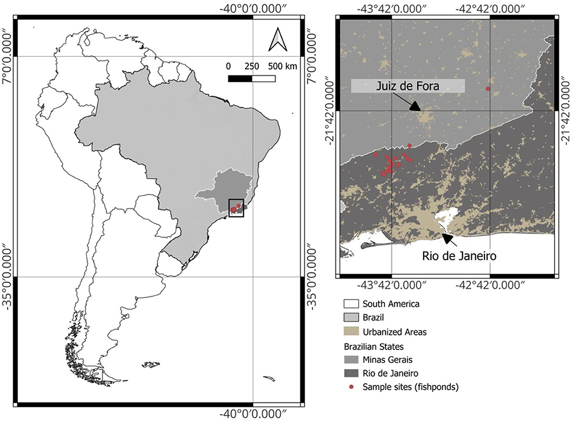
Figure 1. Map of the sampled fish farms (n = 21), located in Rio de Janeiro and Minas Gerais states of Brazil.
2.2. Diffusive flux measurements
In all ponds, CH4 diffusion was measured during daytime using a transparent floating acrylic chamber (29.2 cm inner diameter) connected with gastight tubing (0.4 cm diameter) to a microportable greenhouse gas analyzer (MGGA; ABB—Los Gatos Research, San Jose, CA, USA) in a closed, gastight circuit. Measurements were carried out consecutively in triplicates in the margin and the center of each pond (total n = 6 measurements per pond) and lasted 180s. We used a dinghy with a paddle to navigate the ponds to prevent sediment disturbance. During each triplicate of GHG measurements, we measured air temperature, atmospheric pressure, and wind speed using a portable anemometer (Skymaster Speedtech SM-28, accuracy: 3%). O2 concentrations, temperature, and pH were measured at 50 cm intervals in vertical profiles from the water surface down to the sediment using a Hach HQ40D portable multimeter (Hach, Loveland, CO, USA). CH4 and CO2 fluxes were calculated according to Almeida et al. (2016) using the following equation:
Where F is the gas flux (mg m−2 d−1), V is chamber volume (m3), A is chamber surface area (m2), dC/dt is the change of the measured CH4 or CO2 concentration in time (ppm s−1), P is the atmospheric pressure (atm), M is the molecular mass of CH4 or CO-2 (g mol−1), F1 is a conversion factor of seconds to days (86,400), R is the gas constant (0.082057 L atm−1 K−1 mol−1), and T is atmospheric air temperature (K).
2.3. Ebullitive flux measurements
Ebullitive CH4 fluxes were assessed during 24 h in a subset of 33 ponds. Three bubble traps were installed in the center of each pond. Traps consisted of a funnel (60 cm height, 50 cm diameter) attached to two buoys (empty plastic 500 mL bottles) and to a concrete block that served as an anchor. A 215 mL glass bottle was screwed upside-down on top of the funnel. The traps were filled with water through submersion to capture bubbles in the glass bottles. After ~24 h, the glass bottles were unscrewed and a stopper with a three-way valve was inserted in the bottle while holding it vertically upside down underwater. Subsequently, the volume of the gas phase was determined by adding the required amount of water to fill the bottle. The ebullitive CH4 flux was calculated by multiplying the total gas volume with a CH4 concentration of 48% [based on recent measurements in fish ponds in the same area (n = 22) (Barbosa et al., in preparation1)] and dividing it by the area of the funnel and time of deployment.
2.4. Water sampling and processing
Water samples were taken in triplicate from the water surface in both the margin and the center of each pond. Thirty milliliter of water and 10 mL of atmospheric air were collected in a syringe, which was closed and shaken vigorously for 1 min to equilibrate gas and water CH4 concentrations. Subsequently, 3 mL of gas from the headspace was transferred to a second syringe. This sample was injected into the MGGA in a custom-made setup. This setup was composed of a CO2 filter (a tube containing soda lime) followed by a three-way valve used as the sample inlet, which was then connected with gastight tubing to the MGGA inlet. The CH4 concentrations (ctot) in the water phase were calculated as follows:
Where cgas, cwater, and catm are the CH4 concentrations (mg L−1) in the gas and water phase, and in the atmosphere during water sampling (as measured by the GGA) and Vgas and Vwater are the volumes (L) of the gas and water phase, respectively. The concentration in the water phase was calculated according to Sander (2015):
Henry's volatility is calculated accordingly:
Where kH (mol L−1 atm−1) is calculated as follows:
Where is Henry's constant (for CH4: 1.4*10−3 mol L−1 atm−1), is 1,600 K.
One additional water sample was taken at the water surface of both the margin and the center of each pond to determine Chlorophyll (Chl) a on the same day. A PHYTO-PAM phytoplankton analyzer (Heinz Walz GmbH, Effeltrich, Germany) was used to determine cyanobacteria and green and brown algae concentrations. We used the sum of cyanobacteria and green algae Chl a in our analyses, as the signal for brown algae Chl a is easily distorted by the presence of humic acids or dead algae (Jakob et al., 2005).
In the center of the ponds in which ebullition was determined (n = 31 ponds), we took a sample of the entire water column using a custom-made integrated water sampler consisting of PVC tube with a valve at the bottom, which could be closed underwater by pulling a rope. Water samples were divided into two 10 mL subsamples and stored at −20°C and, after adding 0.1 mL of 65% nitric acid for preservation, at 4°C, until further analysis.
2.5. Sediment sampling and processing
Sediment was taken from the center in all ponds where ebullition was assessed, in case sediment was present (n = 27). A Van Veen sediment grab (Eijkelkamp Soil & Water, Giesbeek, The Netherlands) was used to sample the upper 5–10 cm of sediment, which was placed in vials and stored at 4°C until further processing.
To determine bioavailable nutrients, extractions were carried out using 17.5 g of fresh sediment and 50 mL of demineralized water. After 120 min of incubation on a shaker at 105 rpm, fluid was extracted into a pre-vacuumed syringe connected to a rhizon sampler (Rhizosphere Research Products, Wageningen, The Netherlands). After extraction, samples were divided into three 10 mL subsamples and were either stored at −20°C or stored at 4°C or acidified [adding 0.1 mL of 65% nitric acid (HNO3)] and stored at 4°C, until further chemical analysis (see below). Subsamples of a known volume of fresh sediment were dried at 70°C for 48 h to determine water content and bulk density.
2.6. Sediment incubations
Sediment incubations were carried out to quantify sediment CH4 production potential. Based on the measured in-situ CH4 emission rates, a subset of 20 ponds was selected to cover the entire range of emissions, including the most heterogeneous values. For each of the selected ponds, ~10 g of surface sediment and 30 mL of demineralized water were inserted in a 100 mL glass bottle, using four replicates per pond (n = 80 bottles in total). In one replicate per pond, we glued a non-intrusive planar oxygen-sensitive spot (PreSens Precision Sensing GmbH, Regensburg, Germany) to the inner bottle wall, which could be read out using a compact fiber optic oxygen meter (OXY-1 SMA, PreSens Precision Sensing GmbH, Regensburg, Germany). After closing with a rubber stopper, bottles were flushed with nitrogen gas (N2) for 1 h to create anoxic conditions. We confirmed anoxia by reading out the O2 sensor spots. Bottles were covered in aluminum foil to prevent algal growth and were kept at room temperature. Twice a week, we measured the CH4 concentrations in the headspace of the bottles. Prior to each measurement, bottles were gently swiveled to equilibrate CH4 concentrations in the headspace and water phase. In each bottle, we took a 3 mL sample from the headspace using a syringe, which was injected in the MGGA according to the method described above. Subsequently, we added 3 mL of N2 to the bottles to restore atmospheric pressure. O2 concentrations were assessed in the bottles containing a sensor spot. After measurements on days 15 and 33, bottles were flushed with N2 for 1 h to prevent methanogenesis inhibition by the accumulation of CH4 or other gaseous metabolites in the headspace (Magnusson, 1993; Guérin et al., 2008). The incubations were continued for 43 days.
CH4 concentrations in the bottles were calculated similar to concentrations in water samples (explained above), with the total amount of CH4 per bottle per gram carbon determined as follows:
Where Vgas and Vwater are the volumes (L) of the gas and water phase, respectively, and TC is the amount of TC in a specific bottle (g). The headspace volume was determined by subtracting the volume of the sediment, calculated from its weight and sediment-specific bulk density, from the total volume of the incubation bottle. CH4 production rates were calculated as follows:
Where P is the production rate during a specific time interval (mmol g C−1 d−1), CH4tot(t-1) is the CH4 concentration at the previous measurement, and Δt is the time between measurements (d). Maximum CH4 production rates (Pmax) were calculated according to Grasset et al. (2019), using a simple logistic model.
2.7. Chemical analyses
Ammonium (), nitrate (), and phosphate () concentrations in the sediment extraction and surface water subsamples stored at −20°C were determined by colorimetric methods (Auto Analyser III, Bran and Luebbe GmbH, Norderstedt, Germany). In the acidified subsamples, P and iron (Fe) were measured using inductively coupled plasma optical emission spectrometry (ICP-OES) (Thermo Fischer Scientific, Bremen, Germany).
Total carbon (TC) was measured using 150 mg of dry sample, by high-temperature catalytic oxidation in a Shimadzu TOC analyzer equipped with a solid combustion system (TOC/L ASI-L, SSM 5000).
2.8. Statistical analyses
Statistics were performed using R version 4.0.3 (R Core Team, 2020) and the package psych (Revelle, 2023). Figures were made using ggplot2 (Wickham, 2016). Replicates of CH4 ebullition rates, diffusion rates and CH4 concentrations were averaged for each pond per location within the pond (center or margin). Paired samples t-tests were performed to compute the difference between ebullition and diffusion (after log-transformation of both variables) and between margin and center diffusive emissions and CH4 concentration. Relations between CH4 diffusion, ebullition, and Pmax were tested using linear regression. Model assumptions were validated using Q-Q plots, variance plots, and Shapiro-Wilk tests. Principal component analysis (PCA) was used to explore relationships between environmental variables and CH4 emissions from pond centers. As diffusion and ebullition datasets differed in size, and as we expected different drivers, with diffusion and concentration mostly driven by water phase parameters, and ebullition and Pmax by sediment parameters, we carried out two separate PCAs. The PCA covering CH4 diffusion and concentration included explanatory variables surface water pH, O2, Chl a concentration, N ( + ), , pond depth and pond surface area. For the model of ebullition and Pmax, we included sediment pH, N, and Fe concentrations, depth, and surface area. Variables were log-transformed if skewness exceeded 2 or if the min-max ratio was below 0.1 (Sobek et al., 2007). PCA results were visualized in biplots.
3. Results
3.1. Ebullition was the main CH4 emission pathway
Ebullitive CH4 emissions ranged between 0 and 477 mg m−2 d−1 (median: 76 mg m−2 d−1, average: 115 mg m−2 d−1), and exceeded diffusive emissions in 25 out of 31 ponds (Figure 2). Ebullitive emissions were significantly higher than diffusive emissions (paired samples t-test, df = 29, t = 4.21, p < 0.001). Ebullition contributed 0–99% to total CH4 emissions (diffusion + ebullition), with a median of 85%, and an average of 72%. The highest ebullitive emissions were measured in the concrete pond, which was being drained during the measurements. Because of these conditions, this pond was excluded from further analyses. In the ponds where the sediment layer was too thin to be collected with our sediment grab, ebullition rates were low (median 13 mg CH4 m−2 d−1, n = 4). In several cases, within-pond spatial variation was high, with maximum 210 mg m−2 d−1 difference between the lowest and the highest measurement. Although the ebullitive CH4 emissions in our ponds were generally high, some of the values are underestimated due to exceedance of the maximum gas volume (215 mL; nine bubble traps in three ponds, see Figure 2) during the 24 h sampling time. These ponds were excluded from further statistical analyses.
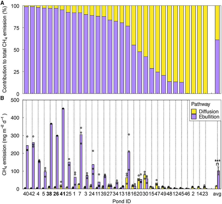
Figure 2. CH4 diffusion and ebullition in 31 fishponds. (A) Contribution of diffusion and ebullition to total CH4 emissions and (B) Diffusive and ebullitive CH4 emissions measured in the center of the ponds. Bars represent average emissions. Gray dots represent individual measurements (n = 3) and may overlap. Only ponds in which both emission pathways were quantified are depicted here (n = 31). Bars are sorted from high to low ebullition contribution, with “avg” representing the averages over all ponds, error bars depicting standard errors, and *** representing significance level p < 0.001 (paired samples t-test). The pond IDs printed in bold are the ponds where the ebullitive flux may have been underestimated due to exceedance of the maximum capacity of the bubble traps.
3.2. Diffusive CH4 emissions were generally low and varied spatially
Diffusive CH4 emissions from the ponds were highly variable, with average center emissions ranging from 2.2 to 86 mg CH4 m−2 d−1 (median: 11 mg m−2 d−1, average: 19 mg m−2 d−1, n = 48) (Figure 3). Emissions at the margins were almost two times lower (paired samples t-test, df = 47, t = −5.52, p < 0.001): ranging from 0.7 to 67 mg m−2 d−1 (median: 6.1 mg m−2 d−1, average: 12 mg m−2 d−1, n = 48). Diffusive emissions were positively related to surface water CH4 concentrations (linear regression, df = 91, F = 50.19, p < 0.001), but not related to CH4 ebullition (linear regression, df = 29, F = 0.33, p = 0.57). Surface water CH4 concentrations ranged between 0.002 and 15.63 μmol L−1 (median: 0.42 μmol L−1, average: 1.46 μmol L−1), but did not differ between pond centers and margins (paired samples t-test, df = 45, t = 0.74, p = 0.46).
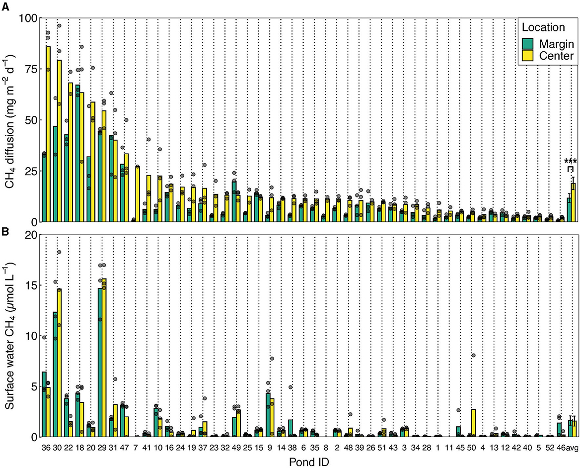
Figure 3. CH4 diffusion and surface water CH4 concentrations in fishponds. (A) Diffusive CH4 emissions and (B) surface water CH4 concentrations at the margin and center of the fishponds. Emissions are sorted from high to low center diffusive emissions. Bars represent average values per pond. Gray dots indicate individual measurements (n = 3) and may overlap. Only ponds in which both center and margin emissions could be quantified are included (n = 47). Bars are sorted from high to low diffusion in the center of the pond, with “avg” representing the average fluxes over all ponds, error bars depicting standard errors, and *** representing significance level p < 0.001 (paired samples t-test).
3.3. Sediment CH4 production
CH4 production in fishpond sediments started immediately after incubation, with the highest increase in headspace CH4 concentrations occurring between 22 and 33 days (Figure 4). Pmax ranged between 0 and 3.17 mg CH4 g C−1 d−1, with an average of 0.64 mg CH4 g C−1 d−1. Pmax did not correlate significantly with CH4 ebullition (linear regression, df = 16, t = 0.83, p = 0.428) or diffusion (linear regression, df = 16, t = −1.61, p = 0.127).
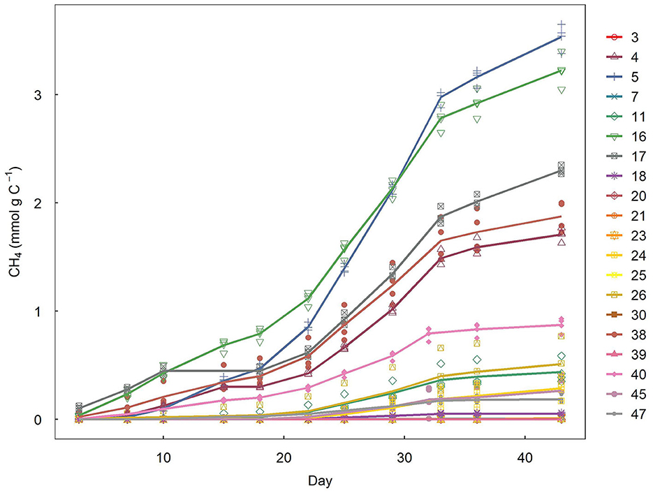
Figure 4. Cumulative CH4 emissions from incubated sediments. Symbols represent individual incubation bottle replicates retrieved from individual ponds; lines represent average trends per pond. Numbers refer to pond IDs.
3.4. Environmental variables differed substantially between ponds
Fishponds were highly variable in surface water O2 concentration, pH and algae concentrations, indicating big differences in trophic state (Table 1). Surface water N was below 50 μmol L−1 in 34 ponds, but 5 ponds had very high concentrations, up to 1,068 μmol L−1. Surface water concentrations were below 10 μmol L−1 in all ponds. In the sediment, N concentrations were generally high, up to 4,526 μmol kg dw−1. Sediment concentrations were nihil in all but six ponds, which had concentrations up to 47.2 μmol kg dw−1. PCA analyses (Figure 5) indicate that CH4 ebullition was positively correlated to sediment N concentration, and Pmax was correlated negatively to sediment Fe content and positively to sediment pH. CH4 diffusion and concentration were negatively correlated to surface water pH and O2 and depth.

Table 1. Summary of environmental variables measured in the fishponds.
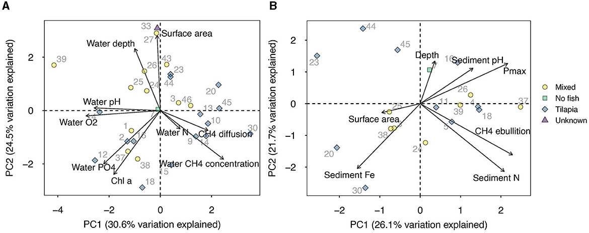
Figure 5. PCA of (A) CH4 diffusion and concentration and environmental variables related to surface water and (B) CH4 ebullition and sediment Pmax and environmental variables related to sediment.
4. Discussion
4.1. Ebullition as a major CH4 emission pathway in fishponds
Ebullition was the main CH4 emission pathway in 81% of the fishponds in our study, contributing 85% (median) to the total CH4 emission. In more than half of the ponds, the contribution of ebullition exceeded the 42–77% ebullition contribution previously found in mesocosm studies with fish (Davidson et al., 2018; Oliveira Junior et al., 2019), which were used in the recent aquaculture footprint estimate by Kosten et al. (2020). Our findings suggest that high contributions of CH4 ebullition to total emissions identified in previous studies on freshwater fishponds (Flickinger et al., 2020; Zhao et al., 2021; Waldemer and Koschorreck, 2023; Yang et al., 2023) are not exceptional, and dominance of ebullition over diffusion may indeed be widespread. However, we also found fishponds with very low ebullition rates, corresponding with very low total CH4 emissions.
The contribution of ebullition appears to be higher in our fishponds than in most other freshwater ecosystems (40–60% contribution) (Bastviken, 2009). Although our temporal resolution was only 24 h per pond, our findings were consistent over a large number of ponds sampled during several weeks in locations with similar weather conditions. Our dataset therefore likely includes both hot and cold moments, making it representative for at least the summer months. Furthermore, recent studies found similarly high ebullition contributions in other aquaculture systems (Flickinger et al., 2020; Yuan et al., 2021; Fang et al., 2022). Ebullitive rates can be high in these shallow ponds due to low hydrostatic pressure facilitating bubble release and a short residence time for CH4 oxidation in the water column (e.g., Bastviken, 2009; Natchimuthu et al., 2016). Furthermore, bubble formation is promoted by high sedimentation rates of reactive organic matter (Sobek et al., 2012) which often occur in fishponds due to the high feed input and algae growth. Additionally, our ponds were situated in a tropical climate, where high temperatures, promoting microbial activity, sediment anoxia, and stratification, may even further exacerbate CH4 ebullition (Holgerson et al., 2016). As ebullition has been observed to increase faster with temperature than diffusion, its contribution to total CH4 emissions is expected to be higher in (sub)tropical regions (Aben et al., 2017).
4.2. Fishpond CH4 emissions and environmental variables
The positive correlation of CH4 ebullition with sediment N concentrations may point at an earlier reported (Deemer et al., 2016; DelSontro et al., 2016; Davidson et al., 2018; Beaulieu et al., 2019) link between eutrophication and ebullition rates. Eutrophication and a consequent increase in primary production can enhance CH4 production through increased availability of organic substrate. The observation that ponds that had very little sediment (those ponds where we were not able to collect sediment with our grab), had very low CH4 ebullition is in line with the notion that that sediment accumulation could lead to enhanced CH4 emissions.
Average CH4 diffusive fluxes of 19 mg m−2 d−1 in our pond centers were very low compared to the average of 106 mg m−2 d−1 reported for semi-intensive aquaculture systems (Yuan et al., 2019), suggesting lower CH4 production rates or higher oxidation rates in our systems. Daytime surface water O2 concentrations in our ponds were indeed high, and negatively correlated to CH4 diffusion and concentration, which would support the possibility of water column CH4 oxidation as well as CH4 oxidation in the upper layers of the sediment. The negative correlation of surface water CH4 concentration and diffusion with water depth corroborates with previous findings in small ponds (Holgerson and Raymond, 2016). At a given gas exchange velocity, a shorter distance between the sediment (where most CH4 is generally produced) and the water surface entails a shorter residence time of CH4 in the water column and therefore less time for the CH4 to be oxidized (Bastviken et al., 2008).
Sediment CH4 production potential varied widely between ponds, but did not correlate with in situ CH4 emissions. This underlines the importance of processes occurring in situ, such as surface water characteristics (e.g., O2 availability) and fish activity. A negative link between Pmax and sediment Fe concentration could be explained by the occurrence of Fe reduction in iron rich sediments, which is energetically favorable over methanogenesis (Achtnich et al., 1995; Struik et al., submitted2).
4.3. Spatial variation should be taken into account when measuring CH4 emissions
Spatial variation in CH4 diffusion, with higher emissions from the center than at the margin of ponds, may be explained by differences in sediment depth and sediment particle size distribution. Some ponds contained very little sediment, and these also tended to have low total CH4 emissions. Our ponds were generally slightly deeper in the center than in the margins, which leads to higher sediment accumulation in the center. Furthermore, specifically the finer sediment particles tend to accumulate at the center of a pond (Boyd, 1995), resulting in a higher surface area for microbial biofilm formation (Sanchez et al., 1994). Similar spatial differences in CH4 emissions from feeding zones, aeration zones and margins were found in other aquaculture studies (Yang et al., 2020; Waldemer and Koschorreck, 2023). Spatial variation in sediment depth may also be created by species-specific burrowing and nesting activities of fish, distinct feeding zones, and the location of the pond's water inlets and outlets (Boyd, 1995). Furthermore, sedimentation rates depend on pond age, trophic state, carbon content of the inlet water, drainage frequency, feeding, perimeter-to-surface area ratio and runoff intensity (Boyd, 1995; Brainard and Fairchild, 2012; Holgerson and Raymond, 2016). Measuring CH4 diffusion from only the margin of a pond, which would be the easier option from a logistic viewpoint, could lead to a significant underestimation of whole-pond emissions. For instance, if a pond of 500 m2 (a representative size for our dataset) has a 1-m margin, and the emission in the center is 60% higher than at the margin (the average difference in our measurements), measuring diffusion exclusively at the margin would result in a ~50% underestimation of the whole pond's actual diffusive CH4 emission.
4.4. Implications and recommendations
Farmed fish are currently estimated to have a carbon footprint of 8.8–13.2 kg CO2-eq kg of protein−1, which is much lower than that of pork (43 kg CO2-eq kg of protein−1) or beef (140 kg CO2-eq kg of protein−1) (Pelletier and Tyedmers, 2010; Robb et al., 2017; Hilborn et al., 2018). This footprint estimate, however, is merely based on emissions from infrastructure, and does not include water-atmosphere GHG emissions. A recent conceptual paper added CH4 diffusion and a hypothetical 42–77% contribution of CH4 ebullition to total CH4 emissions (Kosten et al., 2020). This resulted in an aquaculture fish footprint ranging between 48 kg CO2-eq kg of protein−1 (similar to pork) and 111 kg CO2-eq kg of protein−1 (80% of the beef footprint). Our ebullition results further widen the ebullition contribution range (0–99%), unveiling a lot of variation between ponds, regardless of their management type. On the one hand, this implies that a 42–77% contribution may be an underestimation. On the other hand, it shows that low carbon emission aquaculture is possible, which emphasizes the need to understand the drivers and management practices related to CH4 ebullition in fishponds.
Our study captures only a snapshot of each pond, and detailed information about pond management was frequently lacking. Presumably, fish activity considerably influences carbon dynamics, and varies with fish species, density, size, and life stage (e.g., Rahman, 2015; Rutegwa et al., 2019). Furthermore, we may have captured specific hot or cold moments, due to the stochastic, weather-dependent nature of CH4 ebullition. We therefore recommend GHG emission monitoring during the entire production cycle, including pond draining, dredging, and refilling events. Ebullition, the main pathway of fishpond CH4 emissions, should be considered, if not focused on, in all future studies. As both ebullitive and diffusive emissions appear to vary spatially due to sediment dynamics, a sediment distribution map could be used as a basis for a stratified sampling design. Furthermore, eddy covariance techniques may be most suitable to capture both spatiotemporal variation and both emission pathways. Climate-smart management strategies should be studied by focusing on potential trade-offs between eutrophication, CH4 emission and fish production to evaluate the carbon footprint per kg of fish yield. Additionally, energy costs of potential management strategies (e.g., use of aerators or excavators) should weigh up against the achieved GHG emission reduction. Finally, to create a full GHG budget, N2O emissions (Williams and Crutzen, 2010; Hu et al., 2012) and potential carbon burial as a result of photosynthesis (Boyd et al., 2010; Flickinger et al., 2020) should be taken into account. The contribution of carbon burial to the total carbon budget will depend on the ultimate fate of the sediment, as decomposition by drying or reuse as biofertilizer or biogas (Nhut et al., 2019; Drózdz et al., 2020) releases stored carbon back into the atmosphere.
The reduction of GHG emissions from aquaculture by smart management practices is crucial to reduce the greenhouse gas footprint of fish as a sustainable protein source. Our study across many fishponds in a tropical system also shows that fish farming with low carbon emissions is possible. We found very low CH4 emissions in some ponds, including ponds used specifically for commercial production and breeding. As several of these ponds contained very little to no sediment, the prevention of sediment accumulation appears to be an important management tool, as was also suggested by Zhao et al. (2021). Management options include the prevention of overfeeding and excess fertilization and removal of effluent from the bottom instead of the pond's surface. Furthermore, sediment could be collected in designated areas of the pond by creating depressions or by creating currents using aerators (Avnimelech and Ritvo, 2003). Sediment collection results in a lower sediment surface area and facilitates sediment removal. Aeration may further decrease CH4 emissions by enhancing O2 concentrations at the sediment-water interface (Oberle et al., 2019; Yuan et al., 2019), although the increased area of the water-atmosphere interface will enhance the gas exchange velocity of all GHGs (Kosten et al., 2020). In locations where fish farmers are often smallholders, the cost-effectiveness and effective dissemination of climate-smart management practices are crucial for their implementation. Implementing technologies that minimize greenhouse gas emissions and other environmental pollution may well pave the way for farmed fish as a low-footprint, economically sustainable animal protein source.
Data availability statement
The datasets presented in this study can be found in the online repository Archiving and Networked Services (DANS) EASY at https://doi.org/10.17026/dans-zhf-zx7m.
Author contributions
RV: Data curation, Formal analysis, Funding acquisition, Investigation, Methodology, Visualization, Writing—original draft. SK: Conceptualization, Funding acquisition, Methodology, Resources, Supervision, Validation, Writing—review and editing. RA: Data curation, Formal analysis, Funding acquisition, Investigation, Writing—review and editing. RM: Methodology, Writing—review and editing. IM: Investigation, Resources, Writing—review and editing. IB: Investigation, Writing—review and editing. JN: Investigation, Writing—review and editing. EO: Conceptualization, Visualization, Writing—review and editing. AF: Funding acquisition, Writing—review and editing. NB: Conceptualization, Data curation, Funding acquisition, Investigation, Methodology, Project administration, Resources, Supervision, Validation, Writing—review and editing.
Funding
The author(s) declare financial support was received for the research, authorship, and/or publication of this article. This work was supported by the Ecology Fund of the Royal Netherlands Academy of Arts and Sciences. RV was supported by an Incoming Mobility Doctorate Program (PDSR) Grant provided by the University of Juiz de Fora. RA was supported by Cornell Atkinson Postdoctoral Fellowship research funds. SK was supported by NWO-VIDI Grant 203.098. NB received supplemental support from Fundação de Amparo à Pesquisa do Estado de Minas Gerais/FAPEMIG (CRA APQ 02629/21) and CNPq (Grant No. 316265/2021-7).
Acknowledgments
We thank Meredith Holgerson for her advice on statistical methods and Gladson Resende Marques, Germa Verheggen, Sebastian Krosse, José Paranaíba, Gabrielle Quadra, and Anderson Machado for their help in the laboratory and the field.
Conflict of interest
The authors declare that the research was conducted in the absence of any commercial or financial relationships that could be construed as a potential conflict of interest.
Publisher's note
All claims expressed in this article are solely those of the authors and do not necessarily represent those of their affiliated organizations, or those of the publisher, the editors and the reviewers. Any product that may be evaluated in this article, or claim that may be made by its manufacturer, is not guaranteed or endorsed by the publisher.
Supplementary material
The Supplementary Material for this article can be found online at: https://www.frontiersin.org/articles/10.3389/frwa.2023.1256799/full#supplementary-material
Footnotes
1. ^Barbosa, I., Kosten, S., Muzitano, I. S., Nasário, J., Almeida, R. M., Mendonça, R., et al. (in preparation). Greenhouse gas (CH4, N2O, and CO2) emissions from fishponds in Brazil: factors determining spatial and temporal variation.
2. ^Struik, Q., Paranaíba, J. R., Glodowska, M., Kosten, S., Meulepas, B., AB, R.-M., et al. (Submitted). Fe(II)Cl2 Simultaneously Mitigates Eutrophication and Greenhouse Gas Production Through Iron-Dependent Anaerobic Oxidation of Methane.
References
Aben, R. C. H., Barros, N., Van Donk, E., Frenken, T., Hilt, S., Kazanjian, G., et al. (2017). Cross continental increase in methane ebullition under climate change. Nat. Commun. 8, 1–8. doi: 10.1038/s41467-017-01535-y
Achtnich, C., Bak, F., and Conrad, R. (1995). Competition for electron donors among nitrate reducers, ferric iron reducers, sulfate reducers, and methanogens in anoxic paddy soil. Biol. Fertil. Soils 19, 65–72. doi: 10.1007/BF00336349
Almeida, R. M., Nóbrega, G. N., Junger, P. C., Figueiredo, A. V., Andrade, A. S., de Moura, C. G. B., et al. (2016). High primary production contrasts with intense carbon emission in a eutrophic tropical reservoir. Front. Microbiol. 7, e00717. doi: 10.3389/fmicb.2016.00717
Arts, M. T., Ackman, R. G., and Holub, B. J. (2001). “Essential fatty acids” in aquatic ecosystems: a crucial link between diet and human health and evolution. Can. J. Fish. Aquat. Sci. 58, 122–137. doi: 10.1139/f00-224
Avnimelech, Y., and Ritvo, G. (2003). Shrimp and fish pond soils: processes and management. Aquaculture 220, 549–567. doi: 10.1016/S0044-8486(02)00641-5
Bastviken, D. (2009). “Methane,” in: Encyclopedia of Inland Waters, eds G. E. Likens (Oxford: Elsevier), 783–805.
Bastviken, D., Cole, J. J., Pace, M. L., and Van de-Bogert, M. C. (2008). Fates of methane from different lake habitats: connecting whole-lake budgets and CH4 emissions. J. Geophys. Res. Biogeosci. 113, 1–13. doi: 10.1029/2007JG000608
Beaulieu, J. J., DelSontro, T., and Downing, J. A. (2019). Eutrophication will increase methane emissions from lakes and impoundments during the 21st century. Nat. Commun. 10, 1–5. doi: 10.1038/s41467-019-09100-5
Boyd, C. E., Wood, C. W., Chaney, P. L., and Queiroz, J. F. (2010). Role of aquaculture pond sediments in sequestration of annual global carbon emissions. Environ. Pollut. 158, 2537–2540. doi: 10.1016/j.envpol.2010.04.025
Brainard, A. S., and Fairchild, G. W. (2012). Sediment characteristics and accumulation rates in constructed ponds. J. Soil Water Conserv. 67, 425–432. doi: 10.2489/jswc.67.5.425
Canadell, J. G., Monteiro, P. M. S., Costa, M. H., Cotrim da Cunha, L., Cox, P. M., Eliseev, A. V., et al. (2021). “Global carbon and other biogeochemical cycles and feedbacks,” in Climate Change 2021: The Physical Science Basis. Contribution of Working Group I to the Sixth Assessment Report of the Intergovernmental Panel on Climate Change, eds V. Masson-Delmotte, P. Zhai, A. Pirani, S. L. Connors, C. Péan, S. Berger, N. Caud, Y. Chen, L. Goldfarb, M. I. Gomis, M. Huang, K. Leitzell, E. Lonnoy, J. B. R. Matthews, T. K. Maycock, T. Waterfield, O. Yelekçi, R. Yu, and B. Zhou (Cambridge; New York, NY: Cambridge University Press), 673–816.
Davidson, T. A., Audet, J., Jeppesen, E., Landkildehus, F., Lauridsen, T. L., Søndergaard, M., et al. (2018). Synergy between nutrients and warming enhances methane ebullition from experimental lakes. Nat. Clim. Chang. 8, 156–160. doi: 10.1038/s41558-017-0063-z
Deemer, B. R., Harrison, J. A., Li, S., Beaulieu, J. J., DelSontro, T., Barros, N., et al. (2016). Greenhouse gas emissions from reservoir water surfaces: a new global synthesis. Bioscience 66, 949–964. doi: 10.1093/biosci/biw117
DelSontro, T., Boutet, L., St-Pierre, A., del Giorgio, P. A., and Prairie, Y. T. (2016). Methane ebullition and diffusion from northern ponds and lakes regulated by the interaction between temperature and system productivity. Limnol. Oceanogr. 61, S62–S77. doi: 10.1002/lno.10335
Drózdz, D., Malińska, K., Mazurkiewicz, J., Kacprzak, M., Mrowiec, M., Szczypiór, A., et al. (2020). Fish pond sediment from aquaculture production - current practices and the potential for nutrient recovery: a Review. Int. Agrophysics 34, 33–41. doi: 10.31545/intagr/116394
Fang, X., Wang, C., Zhang, T., Zheng, F., Zhao, J., Wu, S., et al. (2022). Ebullitive CH4 flux and its mitigation potential by aeration in freshwater aquaculture: measurements and global data synthesis. Agric. Ecosyst. Environ. 335, 108016. doi: 10.1016/j.agee.2022.108016
Flickinger, D. L., Costa, G. A., Dantas, D. P., Proença, D. C., David, F. S., Durborow, R. M., et al. (2020). The budget of carbon in the farming of the Amazon river prawn and tambaqui fish in earthen pond monoculture and integrated multitrophic systems. Aquac. Reports 17, 100340. doi: 10.1016/j.aqrep.2020.100340
Grasset, C., Abril, G., Mendonça, R., Roland, F., and Sobek, S. (2019). The transformation of macrophyte-derived organic matter to methane relates to plant water and nutrient contents. Limnol. Oceanogr. 64, 1737–1749. doi: 10.1002/lno.11148
Guérin, F., Abril, G., de Junet, A., and Bonnet, M. P. (2008). Anaerobic decomposition of tropical soils and plant material: implication for the CO2 and CH4 budget of the Petit Saut Reservoir. Appl. Geochem. 23, 2272–2283. doi: 10.1016/j.apgeochem.2008.04.001
Henchion, M., Hayes, M., Mullen, A. M., Fenelon, M., and Tiwari, B. (2017). Future protein supply and demand: strategies and factors influencing a sustainable equilibrium. Foods 6, 1–21. doi: 10.3390/foods6070053
Hicks, C. C., Cohen, P. J., Graham, N. A. J., Nash, K. L., Allison, E. H., D'Lima, C., et al. (2019). Harnessing global fisheries to tackle micronutrient deficiencies. Nature 574, 95–98. doi: 10.1038/s41586-019-1592-6
Hilborn, R., Banobi, J., Hall, S. J., Pucylowski, T., and Walsworth, T. E. (2018). The environmental cost of animal source foods. Front. Ecol. Environ. 16, 329–335. doi: 10.1002/fee.1822
Holgerson, M. A., and Raymond, P. A. (2016). Large contribution to inland water CO2 and CH4 emissions from very small ponds. Nat. Geosci. 9, 222–226. doi: 10.1038/ngeo2654
Holgerson, M. A., Zappa, C. J., and Raymond, P. A. (2016). Substantial overnight reaeration by convective cooling discovered in pond ecosystems. Geophys. Res. Lett. 43, 8044–8051. doi: 10.1002/2016GL070206
Hu, Z., Lee, J. W., Chandran, K., Kim, S., and Khanal, S. K. (2012). Nitrous oxide (N2O) emission from aquaculture: a review. Environ. Sci. Technol. 46, 6470–6480. doi: 10.1021/es300110x
IPCC (2019). 2019 Refinement to the 2006 IPCC Guidelines for National Greenhouse Gas Inventories, eds E. Calvo Buendia, K. Tanabe, A. Kranjc, J. Baasansuren, M. Fukuda, S. Ngarize, A. Osako, Y. Pyrozhenko, P. Shermanau, and S. Federici (IPCC).
Jakob, T., Schreiber, U., Kirchesch, V., Langner, U., and Wilhelm, C. (2005). Estimation of chlorophyll content and daily primary production of the major algal groups by means of multiwavelength-excitation PAM chlorophyll fluorometry: performance and methodological limits. Photosynth. Res. 83, 343–361. doi: 10.1007/s11120-005-1329-2
Kawarazuka, N. (2010). “The contribution of fish intake, aquaculture, and small-scale fisheries to improving food and nutrition security: A literature review,” WorldFish Working Paper No.2106. Penang, Malaysia.
Kosten, S., Almeida, R. M., Barbosa, I., Mendonça, R., Santos Muzitano, I., Sobreira Oliveira-Junior, E., et al. (2020). Better assessments of greenhouse gas emissions from global fish ponds needed to adequately evaluate aquaculture footprint. Sci. Total Environ. 748, 141247. doi: 10.1016/j.scitotenv.2020.141247
Magnusson, T. (1993). Carbon dioxide and methane formation in forest mineral and peat soils during aerobic and anaerobic incubations. Soil Biol. Biochem. 25, 877–883. doi: 10.1016/0038-0717(93)90090-X
Natchimuthu, S., Sundgren, I., Gålfalk, M., Klemedtsson, L., Crill, P., Danielsson, Å., et al. (2016). Spatio-temporal variability of lake CH 4 fluxes and its influence on annual whole lake emission estimates. Limnol. Oceanogr. 61, S13–S26. doi: 10.1002/lno.10222
Nhut, N., Hao, N. V., Bosma, R. H., Verreth, J. A. V., Eding, E. H., and Verdegem, M. C. J. (2019). Options to reuse sludge from striped catfish ( Pangasianodon hypophthalmus, Sauvage, 1878) ponds and recirculating systems. Aquac. Eng. 87, 102020. doi: 10.1016/j.aquaeng.2019.102020
Oberle, M., Salomon, S., Ehrmaier, B., Richter, P., Lebert, M., and Strauch, S. M. (2019). Diurnal stratification of oxygen in shallow aquaculture ponds in central Europe and recommendations for optimal aeration. Aquaculture 501, 482–487. doi: 10.1016/j.aquaculture.2018.12.005
Oliveira Junior, E. S., Temmink, R. J. M., Buhler, B. F., Souza, R. M., Resende, N., Spanings, T., et al. (2019). Benthivorous fish bioturbation reduces methane emissions, but increases total greenhouse gas emissions. Freshw. Biol. 64, 197–207. doi: 10.1111/fwb.13209
Pelletier, N., and Tyedmers, P. (2010). Life cycle assessment of frozen tilapia fillets from indonesian lake-based and pond-based intensive aquaculture systems. J. Ind. Ecol. 14, 467–481. doi: 10.1111/j.1530-9290.2010.00244.x
R Core Team (2020). R: A Language and Environment for Statistical Computing. Vienna: R Foundation for Statistical Computing. Available online at: https://www.r-project.org/
Rahman, M. M. (2015). Role of common carp (Cyprinus carpio) in aquaculture production systems. Front. Life Sci. 8, 1045629. doi: 10.1080/21553769.2015.1045629
Revelle, W. (2023). psych: Procedures for Psychological, Psychometric, and Personality Research. R package version 2.3.6. Evanston, IL: Northwestern University. Available online at: https://CRAN.R-project.org/package=psych
Robb, D. H. F., MacLeod, M., Hasan, M. R., and Soto, D. (2017). Greenhouse Gas Emissions From Aquaculture: a Life Cycle Assessment of Three Asian Systems. FAO Fisheries and Aquaculture Technical Paper No. 609 (Rome: FAO), 110.
Rutegwa, M., Gebauer, R., Veselý, L., Regenda, J., Strunecký, O., Hejzlar, J., et al. (2019). Diffusive methane emissions from temperate semi-intensive carp ponds. Aquac. Environ. Interact. 11, 19–30. doi: 10.3354/aei00296
Sanchez, J. M., Arijo, S., Muñoz, M. A., Moriñigo, M. A., and Borrego, J. J. (1994). Microbial colonization of different support materials used to enhance the methanogenic process. Appl. Microbiol. Biotechnol. 41, 480–486. doi: 10.1007/BF00939040
Sander, R. (2015). Compilation of Henry's law constants (version 4.0) for water as solvent. Atmos. Chem. Phys. 15, 4399–4981. doi: 10.5194/acp-15-4399-2015
Sobek, S., Delsontro, T., Wongfun, N., and Wehrli, B. (2012). Extreme organic carbon burial fuels intense methane bubbling in a temperate reservoir. Geophys. Res. Lett. 39, 2–5. doi: 10.1029/2011GL050144
Sobek, S., Tranvik, L. J., Prairie, Y. T., Kortelainen, P., and Cole, J. J. (2007). Patterns and regulation of dissolved organic carbon: an analysis of 7,500 widely distributed lakes. Limnol. Oceanogr. 52, 1208–1219. doi: 10.4319/lo.2007.52.3.1208
Tong, C., Bastviken, D., Tang, K. W., Yang, P., Yang, H., Zhang, Y., et al. (2021). Annual CO2 and CH4 fluxes in coastal earthen ponds with Litopenaeus vannamei in southeastern China. Aquaculture 545, 737229. doi: 10.1016/j.aquaculture.2021.737229
Vasanth, M., Muralidhar, M., and Saraswathy, R. (2016). Methodological approach for the collection and simultaneous estimation of greenhouse gases emission from aquaculture ponds. Environ. Monit. Assess. 188, 671. doi: 10.1007/s10661-016-5646-z
Waldemer, C., and Koschorreck, M. (2023). Spatial and temporal variability of greenhouse gas ebullition from temperate freshwater fish ponds. Aquaculture 574, 739656. doi: 10.1016/j.aquaculture.2023.739656
Whiting, G. J., and Chanton, J. P. (1993). Primary production control of methane emission from wetlands. Nature 364, 794–795. doi: 10.1038/364794a0
Williams, J., and Crutzen, P. J. (2010). Nitrous oxide from aquaculture. Nat. Publ. Gr. 3, 143. doi: 10.1038/ngeo804
Wu, S., Hu, Z., Hu, T., Chen, J., Yu, K., Zou, J., et al. (2018). Annual methane and nitrous oxide emissions from rice paddies and inland fish aquaculture wetlands in southeast China. Atmos. Environ. 175, 135–144. doi: 10.1016/j.atmosenv.2017.12.008
Yang, P., Tang, K. W., Yang, H., Tong, C., Zhang, L., Lai, D. Y. F., et al. (2023). Contrasting effects of aeration on methane (CH4) and nitrous oxide (N2O) emissions from subtropical aquaculture ponds and implications for global warming mitigation. J. Hydrol. 617, 128876. doi: 10.1016/j.jhydrol.2022.128876
Yang, P., Zhang, Y., Yang, H., Guo, Q., Lai, D. Y. F., Zhao, G., et al. (2020). Ebullition was a major pathway of methane emissions from the aquaculture ponds in southeast China. Water Res. 184, 116176. doi: 10.1016/j.watres.2020.116176
Yuan, J., Liu, D., Xiang, J., He, T., Kang, H., and Ding, W. (2021). Methane and nitrous oxide have separated production zones and distinct emission pathways in freshwater aquaculture ponds. Water Res. 190, 116739. doi: 10.1016/j.watres.2020.116739
Yuan, J., Xiang, J., Liu, D., Kang, H., He, T., Kim, S., et al. (2019). Rapid growth in greenhouse gas emissions from the adoption of industrial-scale aquaculture. Nat. Clim. Chang. 9, 318–322. doi: 10.1038/s41558-019-0425-9
Keywords: greenhouse gases, fishponds, diffusion, tilapia, sediment, mitigation, food production, fish farming
Citation: Vroom RJE, Kosten S, Almeida RM, Mendonça R, Muzitano IS, Barbosa I, Nasário J, Oliveira Junior ES, Flecker AS and Barros N (2023) Widespread dominance of methane ebullition over diffusion in freshwater aquaculture ponds. Front. Water 5:1256799. doi: 10.3389/frwa.2023.1256799
Received: 11 July 2023; Accepted: 15 September 2023;
Published: 13 October 2023.
Edited by:
Ralf Kiese, Karlsruhe Institute of Technology (KIT), GermanyReviewed by:
Tao Huang, Nanjing Normal University, ChinaAlain Isabwe, University of Michigan, United States
Copyright © 2023 Vroom, Kosten, Almeida, Mendonça, Muzitano, Barbosa, Nasário, Oliveira Junior, Flecker and Barros. This is an open-access article distributed under the terms of the Creative Commons Attribution License (CC BY). The use, distribution or reproduction in other forums is permitted, provided the original author(s) and the copyright owner(s) are credited and that the original publication in this journal is cited, in accordance with accepted academic practice. No use, distribution or reproduction is permitted which does not comply with these terms.
*Correspondence: Renske J. E. Vroom, renske.vroom@ru.nl