 Rachel Kaitlyn Uecker
 Brady Adams Flinchum
 W. Steven Holbrook
 Bradley James Carr
- 1Department of Environmental Engineering and Earth Sciences, Clemson University, Clemson, SC, United States
- 2Department of Geosciences, Virginia Tech, Blacksburg, VA, United States
- 3Department of Geology and Geophysics, University of Wyoming, Laramie, WY, United States
Physical, chemical, and biological processes create and maintain the critical zone (CZ). In weathered and crystalline rocks, these processes occur over 10–100 s of meters and transform bedrock into soil. The CZ provides pore space and flow paths for groundwater, supplies nutrients for ecosystems, and provides the foundation for life. Vegetation in the aboveground CZ depends on these components and actively mediates Earth system processes like evapotranspiration, nutrient and water cycling, and hill slope erosion. Therefore, the vertical and lateral extent of the CZ can provide insight into the important chemical and physical processes that link life on the surface with geology 10–100 s meters below. In this study, we present 3.9 km of seismic refraction data in a weathered and crystalline granite in the Laramie Range, Wyoming. The refraction data were collected to investigate two ridges with clear contrasts in vegetation and slope. Given the large contrasts in slope, aspect, and vegetation cover, we expected large differences in CZ structure. However, our results suggest no significant differences in large-scale (>10 s of m) CZ structure as a function of slope or aspect. Our data appears to suggest a relationship between LiDAR-derived canopy height and depth to fractured bedrock where the tallest trees are located over regions with the shallowest depth to fractured bedrock. After separating our data by the presence or lack of vegetation, higher P-wave velocities under vegetation is likely a result of higher saturation.
Introduction
The critical zone (CZ) has been defined as the region extending from the top of vegetation to bedrock (Brantley et al., 2007; Befus et al., 2011; Riebe et al., 2017). Here, physical, chemical, and biological processes work together to transform bedrock into soil (Anderson et al., 2013; Brantley et al., 2017; Riebe et al., 2017). Regolith is the weathered material separating the soil and unaltered bedrock layer. Bedrock topography is a physical boundary below the surface that divides unweathered bedrock and regolith and is used to define the CZ (Rempe and Dietrich, 2014; Flinchum et al., 2018b). Meteoric water and the atmosphere interact with fresh bedrock, driving physical and chemical weathering and creating porosity (Brantley et al., 2007; Rempe and Dietrich, 2014; Hasenmueller et al., 2017; Riebe et al., 2017). Subsurface CZ structures provide essential pore space for water storage (Graham et al., 2010; Flinchum et al., 2018a; Callahan et al., 2022), influences flow paths of groundwater (Goodfellow et al., 2016), supply nutrients for ecosystems (Hahm et al., 2014) and provides the foundation for life (Anderson et al., 2007; Rempe and Dietrich, 2014; Riebe et al., 2017). Quantifying CZ structure over large spatial scales (100–1,000 s of m) can provide an important perspective and improve our understanding of how chemical, physical, and hydrological processes shape and maintain Earth's critical zone.
In weathered landscapes, the belowground CZ can be 10–100 s of meters thick (Befus et al., 2011; Flinchum et al., 2018b; Holbrook et al., 2019; Eppinger et al., 2021). The CZ can be structurally divided by hydrological properties like flow boundaries (Rempe and Dietrich, 2014), geochemical weathering indices (Brantley et al., 2007; Buss et al., 2013), and physical boundaries (Flinchum et al., 2018b; Holbrook et al., 2019). Traditionally, boreholes have been used to gain access to the CZ and used to define boundaries (Buss et al., 2013; Flinchum et al., 2018b; Holbrook et al., 2019). There are a few examples where boreholes have provided high-resolution information and access to samples for geochemical analysis over the hillslope scale (Anderson et al., 2002; Rempe and Dietrich, 2018), but more often, drilling is constrained by logistical, financial, or site restrictions that limit the number of boreholes that can be drilled to quantify the CZ over large spatial scales. Outcrops and roadcuts offer access and are often used to study CZ boundaries (Ruxton and Berry, 1959; Dethier and Lazarus, 2006; Goodfellow et al., 2014). However, exposures of the full extent of the CZ are rare, may not represent CZ structure throughout the region, and cannot be strategically placed to test process-based hypotheses about CZ evolution. Although we have learned a lot about CZ processes, it remains a challenge to quantify physical variations of structures over hillslope to small watershed scales (~60 acres or 0.3 km2).
Topography impacts how water and temperature are distributed on hillslopes. In ridge and valley systems in the northern hemisphere, north facing slopes are colder and wetter (Branson and Shown, 1990; Anderson et al., 2014; Leone et al., 2020). As a result, north-facing slopes tend to host heavier densities of vegetation than south-facing slopes (Branson and Shown, 1990; Istanbulluoglu et al., 2008; Befus et al., 2011). Alternatively, south-facing slopes are drier, warmer, and experience more freeze and thaw cycles in cold climates. As the ridge slopes weather, steeper north-facing slopes and more gradual southern slopes develop (Branson and Shown, 1990; Istanbulluoglu et al., 2008). Northern slopes in colder climates have heavier snowpacks in winter months that reside longer and melt slower than their south-facing counterparts providing a more sustained flux of water (Branson and Shown, 1990; Istanbulluoglu et al., 2008). Sustained cold conditions have been associated with frost cracking (Anderson et al., 2013, 2014) that, over geologic time, creates thicker regolith. The long-term impact of the asymmetrical vegetation, temperature, and saturation distribution has the potential to impact CZ structure where bedrock is deeper on north-facing slopes (Befus et al., 2011).
Vegetation facilitates the movement of water and nutrients, acting as a bridge between the atmosphere and the CZ (Brantley et al., 2017). Transpiration and photosynthesis are important processes that move water and carbon from the atmosphere into the CZ (McDonnell, 2014). Nutrients are exploited in weathered bedrock, and rock is physically shaped by the chemical processes that occur in the soil surrounding a root system (Schwinning, 2010; Hahm et al., 2014; Dawson et al., 2020). Additionally, trees mediate processes like evapotranspiration, runoff, and erosion (Hasenmueller et al., 2017; Dawson et al., 2020). Trees also physically disturb and break apart solid rock, creating regolith (Roering et al., 2010). Over time, trees overturn regolith through tree throw, possibly impacting long-term erosion rates (Gabet and Mudd, 2010; Roering et al., 2010). Given the connection between vegetation and CZ processes, it is difficult to examine or predict the processes that shape subsurface structures without exploring the role of vegetation and how the two are connected (Roering et al., 2010; Pawlik et al., 2016; Brantley et al., 2017). The CZ controls ecosystem resilience and the presence of trees via the regulation of nutrients and water (Hahm et al., 2014; McCormick et al., 2021). Although the lifespan of a single tree is shorter than the time required for hillslope evolution, it has been shown that trees have a strong relationship with CZ structure (Falco et al., 2019). We want to know if the presence or absence of trees can be used as a variable to predict physical property changes in the CZ at our site. As digital terrain models (DTM) models become more readily available through LiDAR and SFM (Dittmann et al., 2017), quantifying the vegetation height across a given landscape is a spatially exhaustive variable that we can quantify.
We are investigating a site characterized by three small valleys oriented approximately east/west in the Laramie Range, Wyoming. The three valleys are separated by two ridges defining clear north/south facing hillslopes. At our site, the north-facing slopes are steeper than the south-facing slopes. The steeper north-facing slopes are also much more vegetated than the south-facing slopes. We collected on 3.9 km of seismic refraction data to explore subsurface structures and heterogeneity in regions inaccessible to drilling. Given the stark contrast observed by remotely sensed data, we hypothesized significant differences in CZ structure under each hillslope, specifically thicker regolith under the north-facing slopes and thinner regolith under the south-facing slopes. We explored this hypothesis using 3.9 km of seismic refraction data spanning two of the valleys and two of the ridges in the region. Our results suggest no significant differences in CZ structure under the north and south-facing slopes. However, we show that vegetation height, not aspect, weakly correlates to bedrock depth.
Location
Our site is in the Laramie Range in southeastern Wyoming, ~13 km southeast of Laramie, WY (Figure 1). The area is ~0.3 km2 and is at an elevation between 2,400 and 2,500 meters above sea level (Figure 1). We named the site the Three Little Valleys (TLV) because it is characterized by two ridges bound by three valleys. Both ridges present a unique asymmetrical vegetation pattern with heavily vegetated North facing slopes and near bare south-facing slopes (Figure 1). Using light detecting and ranging (LiDAR) data collected in 2015, we were provided with a 0.5 m resolution Digital Elevation Model (DEM), which captures the bare Earth surface, and a 0.5 m resolution Digital Surface Model (DSM), which captures the elevation of all features. To estimate canopy height, we subtract the DSM from the DEM. The site is in the US National Forest, so there are minimal manmade structures within 2–3 km of the study area and none within the bounds of the study area. This is also supported by visible vegetation in the National Agriculture Imagery Program (NAIP) images.
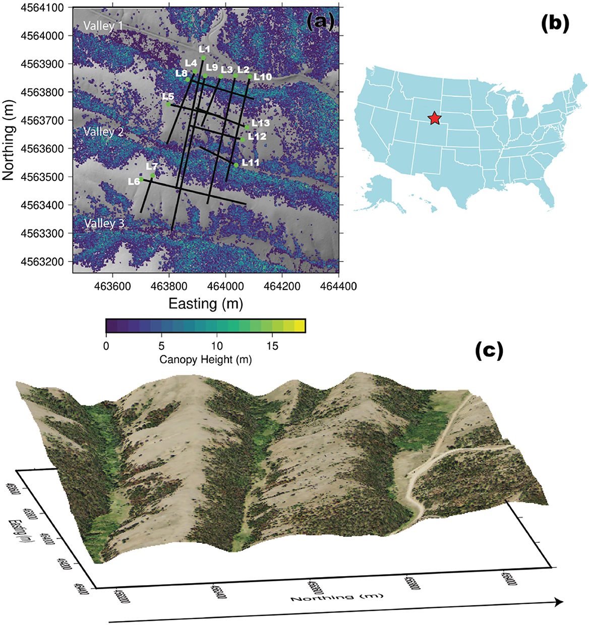
Figure 1. (a) Site map showing shaded topography and canopy height at the Three Little Valleys. Geophysical transects are also shown in black, with the start of the line indicated by a green circle. (b) Inset map showing the location of the site in southeastern Wyoming. Site location is indicated by red stars. (c) 3D map of the site showing differences in slope vegetation and steepness plotted at 2x VE.
On north-facing slopes, canopy height ranges from 1 to 18 meters above the land surface, with the highest vegetation near the valley bottom (Figure 1a). On the south-facing slopes, there is less vegetation, but there are small clusters that can be seen near the valley bottoms with vegetation heights ranging from 1 to 10 meters (Figure 1b). The ground in the region is covered by low-lying sagebrush, and taller vegetation consists of Limber, Ponderosa Pine, Lodgepole Pine, and Aspen Trees (Carey and Paige, 2016; Carey et al., 2019). The valleys at the site are home to small ephemeral creeks that are not monitored. There is a clear difference in slope on the north-facing and south-facing slopes (Figure 1a). The approximate average slope on the north-facing hillslopes is 23%, while on south-facing slopes is 17% (Figure 1).
The Laramie Range is composed of a mid-Proterozoic A-type granite that makes up the Sherman batholith which was uplifted during the Laramide Orogeny (75–55 Ma) (Eggler et al., 1969; Frost et al., 1999). The 1.4 Ga Sherman granite is pink in color with potassium feldspar and biotite composition (Frost et al., 1999). The granite is coarse-grained and weathers to gruss, reaching depths of 60 meters (Eggler et al., 1969). This pattern occurs quickly through wind and water-driven weathering, resulting in undulating topography in the region with scarce outcrops (Eggler et al., 1969). The region has experienced minimal metamorphism since its emplacement, making the composition of the rock at the site relatively uniform (Peterman and Hedge, 1968; Eggler et al., 1969).
TLV is in a snow-dominated system where most of the precipitation comes in the winter as snow. Weather data from the nearby Crow Creek SNOTEL station show that in the last decade, the average annual air temperature has not exceeded 8.9 degrees Celsius or dropped below 1.7 degrees Celsius (National Resource Conservation Service (NRCS 2015). Temperatures are at their lowest in December through March, averaging −5 degrees Celsius, and peak in June through September, averaging 15 degrees Celsius. The annual average precipitation for the area is ~0.6 meters, with 90% of this falling as snow (Natural Resources Conservation Service, 2015).
Methods
Seismic refraction
Seismic refraction is an effective, cost-efficient, and non-invasive geophysical method used to quantify CZ structures. In eroding landscapes underlain by crystalline rock, changes in seismic velocities directly relate to porosity changes caused by either physical or chemical weathering processes (Befus et al., 2011; Flinchum et al., 2018a,b; Holbrook et al., 2019). Seismic velocities are controlled by the bulk modulus, shear modulus, and density of the material (Telford et al., 1990). Variations in these properties occur with changes in depth, resulting in differences in velocity. Theoretical rock physics models have been used to predict P-wave velocities with various input parameters such as porosity, fracture density, effective pressure, composition, and saturation of fluid or gas (see Mavko et al., 2009). However, in an erosional environment underlaid by crystalline bedrock, we expect the chemical and physical weathering process to increase porosity and, as a result, reduce P-wave velocity (Hayes et al., 2019; Callahan et al., 2020). We assume, as others do, that with depth, material becomes less weathered (Befus et al., 2011; Flinchum et al., 2018b; Holbrook et al., 2019).
Seismic refraction is collected using a source to create an elastic disturbance, and geophones record the elastic response. In our case, the source was a sledgehammer striking a steel plate placed on the ground surface. To improve data quality, the shots created by the sound source are stacked to create an average and reduce noise. Geophones were spaced at 1 meter for all lines except Line 1 and Line 2, which had 2.5 and 5 meters spacing, respectively. Shot spacing for the lines varied between 5 and 10 meters for the dataset. We collected 13 individual profiles adding up to a total length of 3.9 km.
We trace-normalized the data and then picked all first arrivals manually. The first arrival was identified at the start of the waveform (Supplementary Figures S2C, D). The picks were made on individual traces using the shot gather as a guide. The one-meter geophone spacing produced high-quality data, and in general, we avoided using filters to pick. However, to pick the arrival times at the farthest offsets, we applied a 50–200 Hz filter (Supplementary Figure S2B). We also used reciprocal travel times to help pick the far offset data to avoid switching phases (Supplementary Figures S2A, B). Given the number of geophones and shots, we knew we would have many arrivals. As a result, we were conservative when picking data. If the arrivals were not clear, they were not picked.
To invert the arrival times, we used the open-source Python Geophysical Inversion and Modeling Library (PyGIMLi) (Rücker et al., 2017). PyGIMLi is based on the shortest path algorithm, which assumes energy travels as rays (Moser, 1991; Moser et al., 1992). The inversion uses a deterministic Gauss-Newton scheme to minimize χ2, which includes uncertainty associated with each pick. The uncertainty for each pick were set using a linear interpolation between 1 and 5 ms as a function of offset. The error of 5 ms occurs at the maximum offset in the survey. This linear assignment of the weights is incorporated because we have more certainty in the near offset picks, and the weights cause the inversion to fit the near offset arrivals better.
The triangular grids for all the models were set up so that there would be at least three model parameters between each geophone at the surface. The model parameters linearly increase with increasing depth to a maximum-size triangle with a side length of 7 m. The model depth varied and was adjusted to ensure enough model parameters to have the rays turn on their own. All initial models used a gradient starting model with 1,000 m/s at the surface and 4,500 m/s at depth. The choice of the higher starting velocity was to force the inversion to put in low-velocity layers. Once low-velocity zones are in place, they are difficult to update and remove from the inversion because rays tend to avoid them. After minimizing the χ2 value we calculated and reported the RMS of the final velocity model.
All inversions had an RMS of <2.5 ms, indicating high-quality inversion fits of our observed travel times (Table 1; Supplementary Figure S3a). Additionally, we had 20 intersection points and used these to check the precision of the inversions before interpretation. To do this, profiles of velocity vs. depth were extracted from both lines at the intersection point where they cross. Each inversion was performed independently of the others, meaning these intersections compared the 2D seismic profiles. When the 1D velocity profiles of the intersections are plotted against each other, they have a slope near 1 (slope = 0.86; R2 = 0.86 Supplementary Figure S3b, c). The near 1:1 values at the intersections support consistent velocity models across the study area.
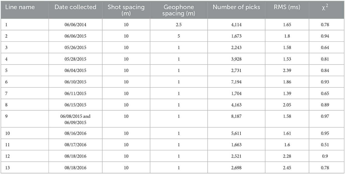
Table 1. Seismic lines and their respective dates collected, shot spacing, geophone spacing, and processing information.
Results
Results of the seismic analysis reveal 3.9 kilometers of subsurface critical zone structure at our study site. In this section, we generalize our observations, but all the individual seismic profile inversions can be found in the Supplementary Figure S1. Near the surface, velocities are ~500 m/s. Although velocity increases with depth, we do not always observe velocities >4,000 m/s (Figure 2). We see higher velocities (>4,000 m/s) closest to the surface under the main valley. Lines that cross the northernmost ridge and then travel across the valley to the southern ridge sometimes show high velocities getting deeper under the ridge and shallower under the valley. In some specific cases, these high velocities appear to be inverted images of the surface topography (Figure 2A). However, not all profiles that cross the valley and ridge show this clear inverted pattern (Lines 1, 4, and 9 in Supplementary Figure S1).
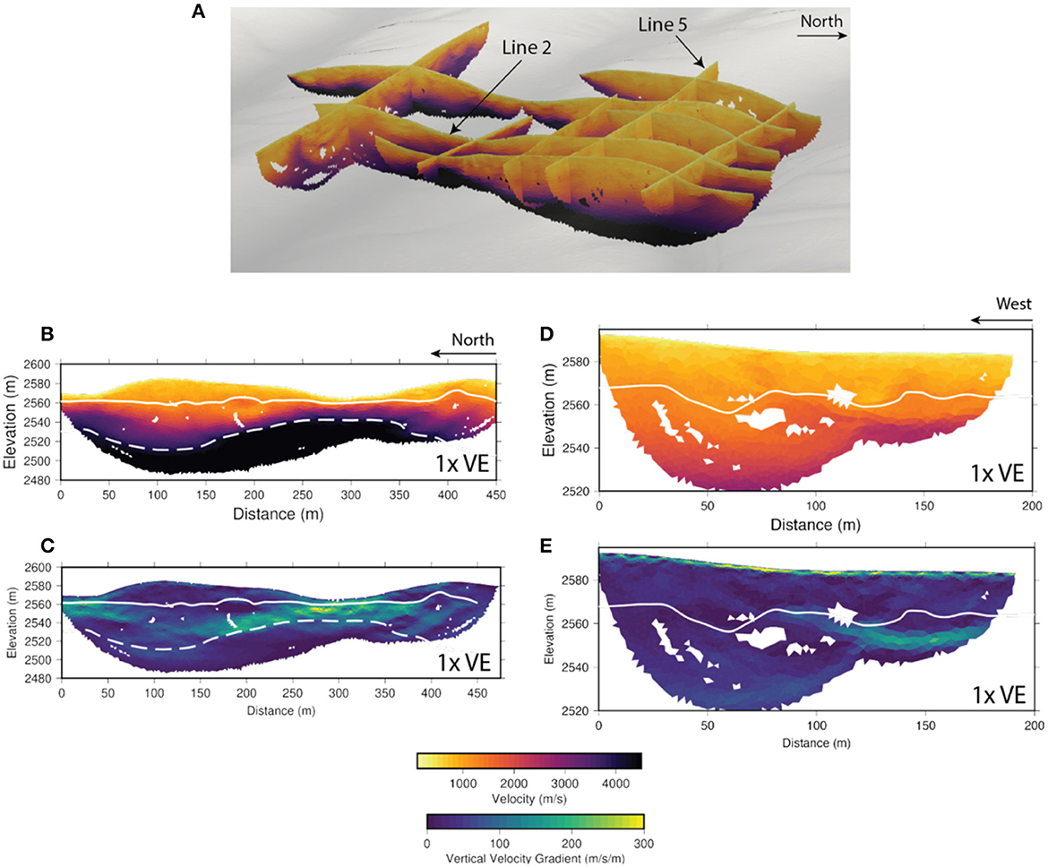
Figure 2. (A) Fence diagram displaying all 3.9 kilometers of inverted seismic velocity data. (B) Seismic results from line 2. This profile crosses both ridges and the central valley. One thousand two hundred and 4,000 m/s velocity contours are shown in solid white and dotted white lines, respectively. (C) Vertical velocity gradient from line 2. (D) Seismic results from line 5 which lies on the southern side of the northern ridge. This profile did not reach high velocities (>4,000 m/s), so only the 1,200 m/s velocity contour is visible. (E) Vertical velocity gradient from line 2. This profile shows a sharp vertical velocity gradient at the soil/saprolite boundary.
We have more lines that cross the northernmost ridge (9 lines vs. four lines on the southern ridge). The northern ridge has a thicker section of velocities <4,000 m/s ridge, with an average depth to the 4,000 m/s contour of 62.02 ± 17.67 m, vs. the southern ridge, with an average depth to the 4,000 m/s contour of 40.32 ± 14.11 m. This pattern can be seen best in line 9, which results from two lines whose ends touched, running perpendicular to the ridges that were inverted together (Line 9 in Supplementary Figure S1). The first 275 meters of the 2D inversion for line 9 represent the northern ridge and show a thick section of velocities <4,000 m/s. Beginning at ~270 meters along this line, glimpses of higher velocities can be seen beneath the central valley and the southern ridge. This pattern can also be seen in Lines 2, 3, and 10 (Supplementary Figure S1).
From the velocity profiles, we calculate the vertical velocity gradient (Figures 2C, E). At locations where the gradient is high, it would support a strong elastic boundary–such as the boundary dividing fractured and fresh bedrock (Huang et al., 2021). Many of our profiles show a continuous and strong vertical gradient near the surface (<1–2 m)–probably indicating the transition from soil to saprolite. There is also a notable vertical gradient (>200 m/s/m) that occurs at depths >15 m in many lines (Lines 2, 3, 5, 8, 9, 10). This vertical velocity gradient occurs right above the high velocities (>4,000 m/s).
Discussion
The results of our seismic survey form the foundation of a comprehensive landscape analysis. The CZ in the TLV is an eroding crystalline environment that can be broken down by material properties determined by the seismic velocities from the survey. These properties can then be used to make inferences about the relationship between surface topography, aspect, and vegetation in the region.
We assume a velocity of 1,200 m/s to define the bottom of dry saprolite and 4,000 m/s as the top of unfractured and unweathered bedrock. These values are based on previous studies where the saprolite boundary is based on the correlation between seismic refraction, geoprobe, and boreholes (Flinchum et al., 2018b; Holbrook et al., 2019). This correlation was made in the Laramie Range on the same granite only 5 km south of our study site. The 4,000 m/s velocity representing fresh bedrock is based on seismic refraction surveys conducted on granite outcrops in the Laramie Range and another on granite in the Southern Sierra Nevada (Holbrook et al., 2014; Flinchum et al., 2018b). We do not have boreholes at this site. However, we define unweathered bedrock as material that is essentially unaltered with some minor chemical weathering and fracturing consistent with other published reports (Befus et al., 2011; Holbrook et al., 2014; Flinchum et al., 2018b). We define weathered bedrock as a material with an intermediate velocity between 1,200 and 4,000 m/s. Based on inspection of optical televiewer data from boreholes <5 km away, the weathered bedrock is material that has some fracturing with some chemical weathering along those fractures (Flinchum et al., 2018b). Finally, saprolite is a material that is extensively fractured and friable but retains the original fabric of the rock (Befus et al., 2011; Flinchum et al., 2018b). Saprolite in crystalline rocks has an average porosity >30% (Flinchum et al., 2018a; Callahan et al., 2020, 2022). Bedrock has a much lower average porosity, about or < 10% (Flinchum et al., 2018a).
The bedrock topography of the region can be seen more clearly when the boundaries for unweathered and weathered bedrock are projected across the entire space. Using the 1,200 and 4,000 m/s velocities, we can construct a 3D three model of the CZ structure under the TLV. Our three-layer model was created by extracting the velocity contours for the saprolite and bedrock boundaries on every profile (Figure 2). The depth of each contour was interpolated across the entire study area using the linear method. Using the LiDAR DEM, we can construct a 3D, three-layer model representing the boundaries for the land surface, weathered bedrock, and unweathered bedrock (Figure 3).
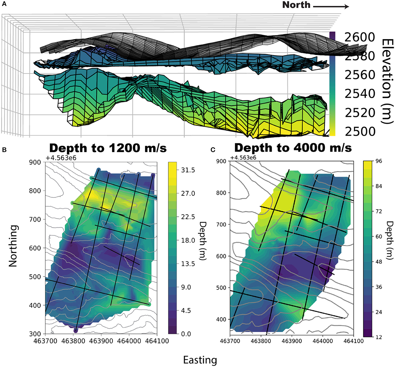
Figure 3. (A) 3D map of the surface, saprolite, and bedrock topography for the site. The colors indicate changes in depth where more yellow colors are deeper, and purple is the shallowest. (B) Map view of the base of saprolite, or the 1,200 m/s boundary with geophysical transects and surface topographic contours shown. (C) Map view of the depth to unweathered bedrock, or the 4,000 m/s boundary with geophysical transects and surface topographic contours shown.
In an eroding crystalline environment, differences in seismic velocity are dominated by changes in porosity which are strongly correlated with weathering (Befus et al., 2011; Flinchum et al., 2018b; Holbrook et al., 2019). However, in the Laramie Range, previous work has found that the water table typically exists near the boundary dividing saprolite and fractured rock (around 2570 meters above sea level at our site) (Flinchum et al., 2018a, 2019). We use 1,200 m/s as the boundary dividing saprolite and fractured rock in this section (Figure 3). The velocity we used to define the top of fractured bedrock (1,200 m/s) is close to the p-wave velocity of water (1,500 m/s). When extracted, the 1,500 m/s surface has an average depth difference between the 1,200 m/s of 4.37 ± 2.98 m (Mean ± 1 standard deviation).
The 3D distribution of the layers provides insight into their lateral variability while providing context by showing the layers relative to the surface topography (Figure 3). We see little topographic variation of the layer defining the base of saprolite (1,200 m/s contour) beneath the northern ridge and central valley. Beneath the southern ridge, this boundary is shallower and appears to mimic the surface topography. The northern ridge sees bedrock depths (4,000 m/s contour) reaching up to 95 meters below the surface, while the southern ridge is far shallower. The map view of these layers provides better insight into the distribution of the layers across the entire region. From the map perspective, we can see that the maximum bedrock depth beneath the northern ridge (~95 m) is concentrated on the western half of the ridge. More shallow bedrock depths (~55 m) are seen on the eastern half of the ridge.
Climate and bedrock
North-facing slopes experience less solar radiation and, as a result, overall cooler conditions in the northern hemisphere (Branson and Shown, 1990; Burnett et al., 2008; Istanbulluoglu et al., 2008). In climates that experience snow, higher elevations (>2,500 m) with north-facing slopes also experience heavier snowpack (Tennant et al., 2017). Land surface structures and vegetation also play an important role in how snow accumulation and ablation in ecosystems occur, and differences in slope and aspect emphasize these (Brooks et al., 2015; Tennant et al., 2017). So, while elevation, temperature, and precipitation play a role in how snow falls, accumulates, and melts in a landscape, north-facing slopes also experience less solar radiation, fewer freeze and thaw cycles, and overall cooler conditions throughout all four seasons (Branson and Shown, 1990; Brooks et al., 2015). These variables, coupled with shade and reduced wind speeds provided by heavier vegetation, result in northern slopes experiencing heavier snow accumulation and more significant melt periods, resulting in spatial and temporal variations in water infiltration (Brooks et al., 2015) between north and south-facing slopes. The harsh cold conditions on north-facing slopes mean they face mechanical damage through frost cracking, when water enters an existing fracture, freezes, and induces weathering (Anderson et al., 2013). Given the distinct contrasts between north and south-facing slopes at our site (Figure 1), we hypothesized large asymmetrical differences in critical zone structure similar to the surface topography. Due to the colder conditions and extensive vegetation coverage on the north-facing slopes, we expected to see a general trend where the weathered material would be deeper on the north-facing slopes.
Using our 3.9 km of seismic data and extracted 1D velocity profiles at every geophone along each line. We used these 1D profiles to infer the general CZ structure under the north and south-facing slopes. The 1D profiles allowed us to sort the data based on the line location, slope, and aspect where the slope and aspect are calculated from the 1 m bare earth LiDAR. We filtered the aspect by excluding east and west-facing values. To do so, we created a 90-degree window facing ± 45 degrees north and ±45 degrees south and removed all data that did not fit this range. To ensure we were investigating velocities under the north or south-facing slopes only, we also removed all data that did not fall on a slope face. This included data in the valley bottoms and along the ridge tops. We did this by removing all 1D profiles that fell on a geophone location with a slope of fewer than 4 degrees (Figure 4A). These two filters left us with 1D velocity profiles located only on north or south-facing slopes.
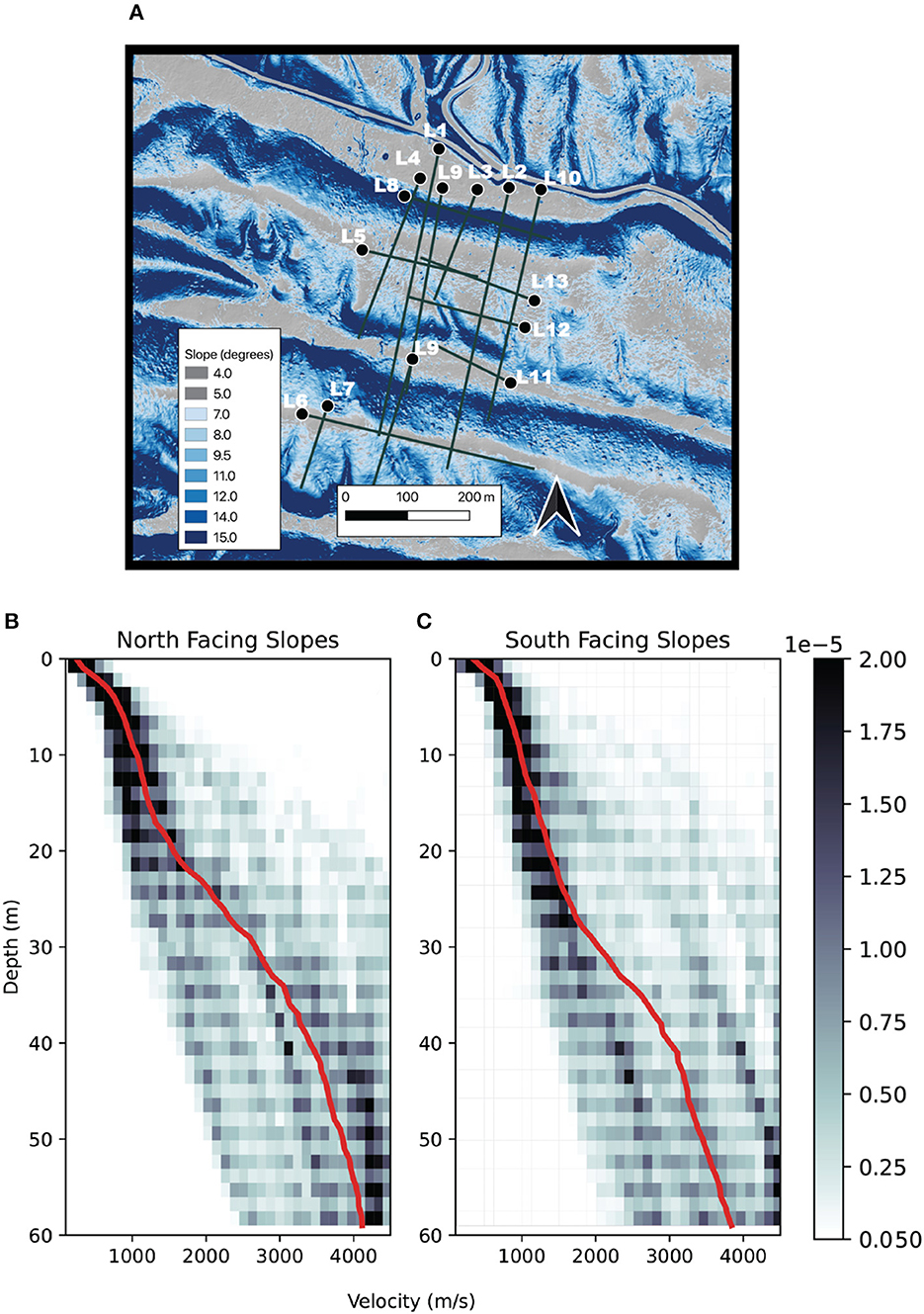
Figure 4. (A) Map of study site with gray areas indicated the aspect regions that were included and excluded from the slope analysis. (B, C) Histogram results of the slope analysis. These plots show the number of times a given velocity occurred at a given depth on both north-facing slopes (left) and south-facing slopes (right). This plot was normalized for visual clarity. Median velocity values across the range of depths are shown in red.
To look for general trends under the north and south-facing slopes, we bin the vertical velocity profiles using 2D histograms (Figure 4). To enable easy comparison between the slopes, we normalized each histogram and then calculated and plotted the median of the data (red line in Figures 4B, C). In the normalized histograms, the area under the surface equals 1. Both north and south-facing slopes start at a velocity of around 500 m/s, increase to 1,200 m/s between depths of 10 and 20 m and then increase to bedrock velocities (Figure 4). Given the huge contrasts in slope and vegetation coverage at the site (Figure 1), the velocity data do not show a significant difference in vertical CZ structure as a function of slope and aspect (Figures 4B, C). One of the only differences is the larger variability that begins between depths of 10–20 m on the north-facing slopes. As the depth increases, it is almost as if the trends on the north-facing slopes are bifurcated with some of the data following a slower increase in velocity with depth, just like the south-facing slopes, and then a subset of the data where the velocity increases more rapidly with depth (Figure 4B). This additional variation is subtle but given the obvious vegetation contrasts (Figure 1), we wondered if the additional variation was caused by two separate velocity trends where vegetation is present or is not present. We will investigate this further in the following sections.
Vegetation and bedrock
To quantify the relationship between vegetation distribution and velocity across the entire site, we used the 1D profiles extracted at each geophone along every profile to determine the depth to the presumed weathered bedrock boundary, or the 1,200 m/s contour (Figure 3B). We averaged the LiDAR data for the canopy height for the site in a 10-meter grid to quantify the distribution of vegetation heights throughout the area. We can use this data to calculate the vegetation height relative to any velocity contour across the site (Figure 5).
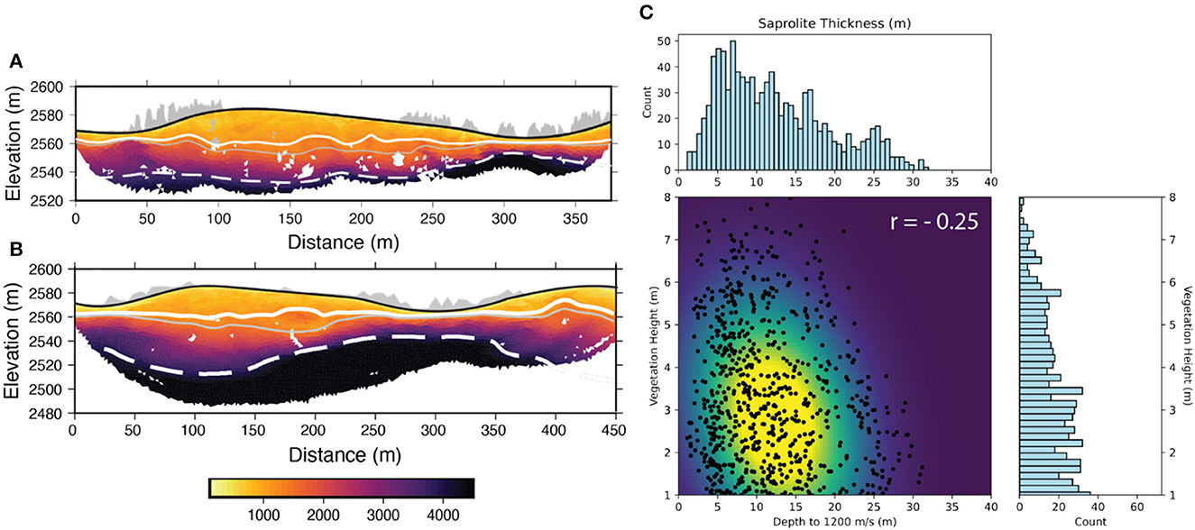
Figure 5. (A, B) Seismic profiles for Lines 10 (A) and 2 (B). Vegetation height along the lines is shown in gray. The solid white line in the profile indicates the velocity contour for 1,200 m/s and the dotted white line indicates the velocity contour for 4,000 m/s. The gray line represents the 1,500 m/s velocity contour. (C) Bivariate distribution plot displaying the relationship between saprolite thickness (m) and vegetation height (m). The variables have a pearson correlation coefficient of −0.25, indicating a weakly negative relationship.
To analyze this relationship, we binned occurrences of different saprolite thicknesses (depth to 1,200 m/s contour) and vegetation heights across the site (Figure 5C). These data were used to produce a bivariate distribution (Figure 5C). This distribution shows a weakly negative relationship (r = −0.25), where the tallest vegetation prefers areas where velocities of 1,200 m/s are shallow (<15–20 m from the surface) or saprolite is thin (Figure 5C). While vegetation height is not always a proxy for species success, we are using heights to characterize the asymmetrical distribution of vegetation across the site and 30 m Landsat NDVI values have too coarse of resolution. With that said, low-lying vegetation like sagebrush (<0.5 m), while present, is considered negligible for this analysis since it is present across the entire region.
Recent work has emphasized the importance of deep structure in providing essential nutrients and water stores for vegetation (Brantley et al., 2017; Dawson et al., 2020; McCormick et al., 2021). In dry climates, trees are particularly dependent on deep bedrock water storage (Dawson et al., 2020; McCormick et al., 2021). A large-scale focus on CZ structure is needed to quantify the relationships between the subsurface and trees truly, but current studies show that the rooting systems of trees are incredibly adept at locating the resources they need (Hahm et al., 2014; Hasenmueller et al., 2017; McCormick et al., 2021). As trees seek out these resources, they modify landscapes through their rooting processes.
In the southern Sierra Nevada mountains, distributions in canopy density were examined using bedrock geochemistry samples, and the granitic batholith was found to have phosphorous quantities under the vegetated areas that were 20 times greater than that of the areas that were bare, pointing to the driving influence of tree distribution to protolith geochemistry (Hahm et al., 2014). The study also pointed to other potential driving forces in tree distribution. This included bedrock weathering, which might influence the water-holding capacity of the rock and density of bedrock fractures which supply the essential footholds and water storage reservoirs for trees. They point out that the regolith's nutrient and water storage (Hahm et al., 2014; Holbrook et al., 2014; Callahan et al., 2020) capacity is dependent on how the protolith weathers, and this can vary even within a geochemically homogeneous space.
Roots tend to find existing fractures and fissures for to access bedrock (Roering et al., 2010; Schwinning, 2010). Root hairs seek out these spaces in search of water and nutrients like phosphorus, sulfur, and potassium (Roering et al., 2010; Hahm et al., 2014). During dry seasons, trees are dependent on water stored at depth in bedrock as shallow soil water reserves become depleted, so the water storage capacity of weathered bedrock is essential for tree growth as it is more dependably accessible throughout the year (Schwinning, 2010; Hasenmueller et al., 2017). Our observations show that the trees have a preference. The trees in TLV could be in areas where the saprolite is thinnest because they are extracting additional nutrients from the less weathered bedrock or because the underlying bedrock forces groundwater flow toward the surface under the drainages. In the next section, we will argue that the trees at TLV show this preference because they are optimally located to have access to water most of the year.
A complex eco-hydrogeologic system
As discussed, the presumed boundary between fractured bedrock (1,200 m/s contour) and an estimate of the water table based on the P-wave velocity of water are quite close across our site, with an average difference of only 4.37 ±2.98 m (Mean ± 1 standard deviation). On our velocity profiles, the difference between 1,200 and 1,500 m/s is not significant at the 1:1 scale (Figures 5A, B). When we repeat the analysis comparing vegetation height to the depth of the 1,500 m/s contour instead of the 1,200 m/s contour, the vegetation trend still holds (Supplementary Figure S5).
It is well-known that P-wave velocities are impacted by saturation, where full saturation will dramatically increase the P-wave velocity (Bachrach and Nur, 1998; Flinchum et al., 2018a). A fully saturated material will have a minimum velocity approaching the velocity of water (1,500 m/s). One possible interpretation is that 1,500 m/s would represent the water table. This means that the gray line seen in Figures 5A, B can be used as a reasonable estimate for the depth of the water table. This suggests that a P-wave velocity of ~1,200–1,500 m/s might represent the transition from saprolite to fractured rock or full saturation. If the water table was located near this transition zone, it would be impossible to tell the difference with P-wave velocity alone.
So, the occurrence of the high velocities in the valley bottoms and the concentration of vegetation in these locations could represent water accessibility—not necessarily the presence of bedrock (velocities > 4,000 m/s). The thick vegetation coverage on the north-facing slopes above the valley bottoms can also be attributed to water accessibility, given the climactic setting of the site. Previous work has shown that heavier and longer-lasting snowpacks, along with denser vegetation, contribute to greater overall moisture retention on the north-facing slopes (Brooks et al., 2015; Tennant et al., 2017). In addition, the area's ridge and valley system likely experiences topographic drainage—meaning water that falls on the highest point of the ridge will drain into the subsurface and toward the valley until it reaches the water table (Brooks et al., 2015). These preferential and natural groundwater flow paths driven by topography would provide additional moisture content on the lower reaches of the slopes near the valley bottoms.
Upon initial investigation, we did not observe significant differences in CZ thickness with variations in slope and aspect (Figure 4). This was surprising given the stark contrast in slope and vegetation coverage of the study area (Figure 1). However, the distribution of velocities on the north-facing slopes is more variable, especially at depths of 5–25 m (Figures 4B, C). At these depths, the north-facing slopes show a slight tendency toward shallower high velocities (Figure 4). In addition, the north-facing slopes almost appear to be a combination of two different distributions superimposed on one another. The first distribution would be like the south-facing slopes (Figure 4C), and the second distribution curve is shifted toward higher velocities. Given our observation that vegetation tends to focus around areas where high velocities are closer to the surface (Figure 5), we wanted to know how or if the vegetation could explain the additional velocity variability in the north-facing slopes. Our hypothesis was that the additional variability in the north-facing slopes might be explained by the presence or lack of vegetation. The north-facing slopes were divided further into two groups: (1) locations where the vegetation height was >1 meter (Figure 6A) and (2) locations where the vegetation was <1 meter (Figure 6B).
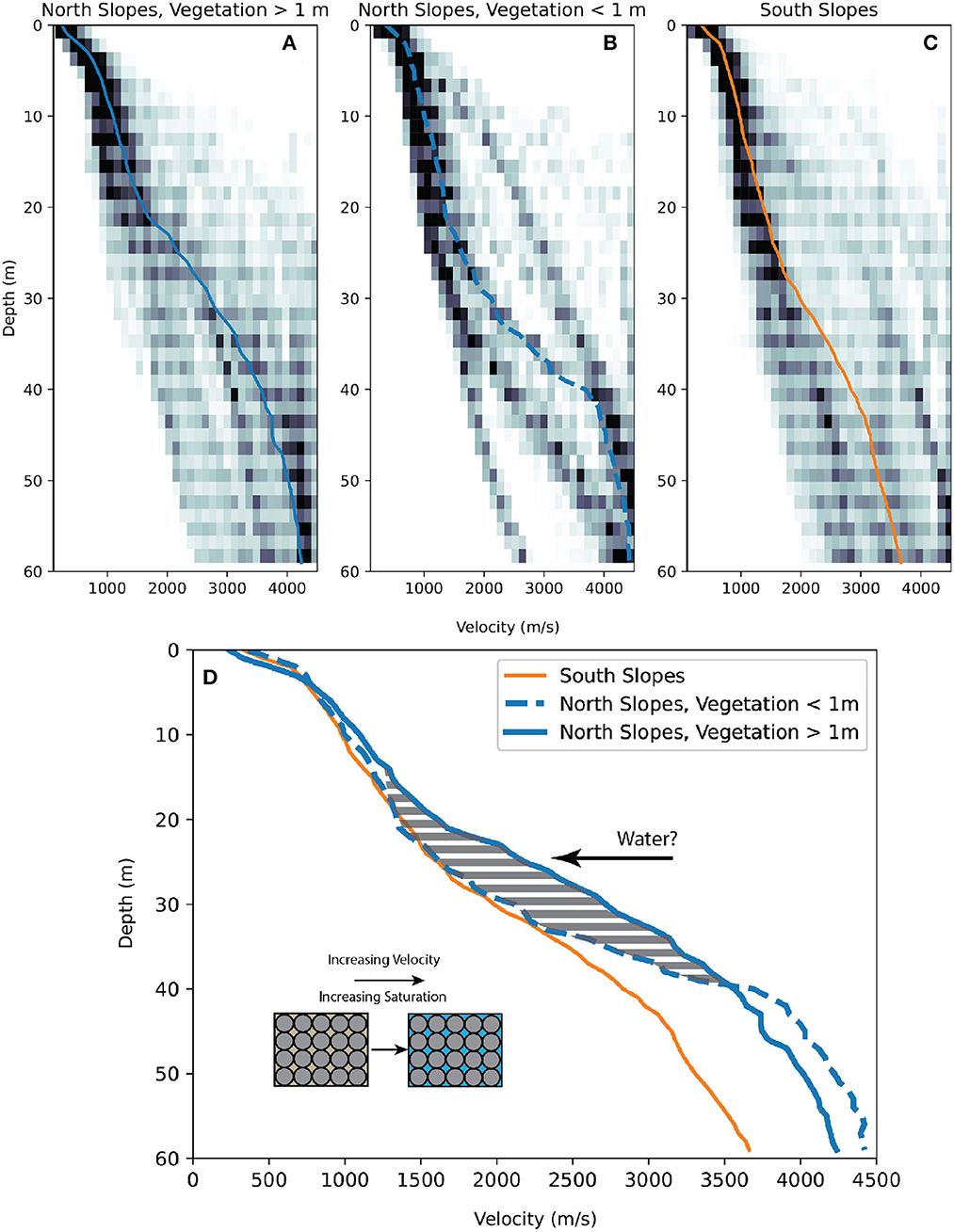
Figure 6. (A) Histogram results of slope analysis with the north-facing slopes separated by vegetation height along with the median of those values shown by the solid blue line. (A) shows north-facing slopes with vegetation >1 meter. (B) Histogram results of north-facing slopes with vegetation <1 meter and a median of those values shown by the dashed blue line. (C) Histogram results of south-facing slopes and a median of those values shown by the solid orange line. (D) Median velocity values of the north-facing slope with and without vegetation and the south-facing slope. Bifurcation of the north facing slope values indicated with gray stripes.
When the north-facing slopes were separated based on their relative canopy height, much of the seismic data associated with taller vegetation concentrated in the shallow (<30 m) subsurface showed a faster trend (Figure 6B). We also see that the data associated with the shorter (<1 m) vegetation show a distribution of velocity to depth that is remarkably like the near bare south-facing slopes (Figures 6C, D). When calculating the p-value between the median values of the datasets, we find that this trend difference has a p-value of <0.05, indicating statistical significance to the separation (Supplementary Figure S4). This makes sense—if the material across the site is geologically homogeneous, full saturation of water will cause a rise in P-wave velocity. Therefore, we can reasonably assume that the preferential growth of trees on the north-facing slopes is a result of high moisture content, causing a slight increase in P-wave velocity.
We expect the valley bottoms to be the most dependable water source in the TLV since they are home to ephemeral streams and are likely the discharge site for topographic drainage between the ridges. The higher density of vegetation and overall cooler conditions on north-facing slopes result in greater overall moisture retention and total groundwater discharge to the valley bottom, making them more hospitable for vegetation growth. The dry, warm south-facing slopes are the least dependable source of water for vegetation, resulting in little growth once upslope of the valley bottom.
Conclusions
The clear difference in aspect, land slope, and vegetation distribution within the Three Little Valleys reveals a complex landscape. The ridge and valley system runs east/west, resulting in north and south-facing slopes. Additionally, the ridges are home to an asymmetrical distribution of vegetation and grade. All these things considered, we expected that the subsurface CZ structure in the TLV would vary with aspect and slope. However, the initial findings of our seismic survey show no clear relationship between slope, aspect, and CZ structure. After filtering our results from the north-facing slopes based on vegetation height, a trend emerges that reveals faster (1,200–1,500 m/s) shallow (5–25 m) velocities are associated with areas with vegetation heights >1 meter. This supports that water is the driving force behind the asymmetrical distribution of vegetation in the Three Little Valleys. In addition, our seismic survey allowed us to quantify bedrock topography over the entire region, revealing areas where unweathered bedrock was undetectable at depths >65 meters and areas where unweathered bedrock was within 20 meters of the surface. This creates a complex eco-hydrogeologic system where trees tend to be located where water is most accessible year-round and that, at least in the Laramie Range, we might be able to use vegetation height as a proxy for understanding how and where groundwater moves through the landscape.
Data availability statement
The processed datasets generated for this study can be found on figshare (https://doi.org/10.6084/m9.figshare.21231329.v1).
Author contributions
RU: seismic data processing and analysis, LiDAR data analysis, and manuscript preparation. BF: data analysis and manuscript preparation. WH: project planning and manuscript preparation. BC: geophysical data collection. All authors contributed to the article and approved the submitted version.
Funding
This project was supported by National Science Foundation grants EAR-2012227, OIA-1208909, and EAR-2012353.
Acknowledgments
We thank Matthew Provart and the many undergraduates who assisted in the field with data collection.
Conflict of interest
The authors declare that the research was conducted in the absence of any commercial or financial relationships that could be construed as a potential conflict of interest.
The reviewer SU declared a past co-authorship with one of the authors BC to the handling Editor.
Publisher's note
All claims expressed in this article are solely those of the authors and do not necessarily represent those of their affiliated organizations, or those of the publisher, the editors and the reviewers. Any product that may be evaluated in this article, or claim that may be made by its manufacturer, is not guaranteed or endorsed by the publisher.
Supplementary material
The Supplementary Material for this article can be found online at: https://www.frontiersin.org/articles/10.3389/frwa.2023.1057725/full#supplementary-material
References
Anderson, R. S., Anderson, S. P., and Tucker, G. E. (2013). Rock damage and regolith transport by frost: an example of climate modulation of the geomorphology of the critical zone: Rock damage and regolith transport by frost. Earth Surf. Process. Landf. 38, 299–316. doi: 10.1002/esp.3330
Anderson, S. P., Dietrich, W. E., and Brimhall, G. H. (2002). Weathering profiles, mass-balance analysis, and rates of solute loss: Linkages between weathering and erosion in a small, steep catchment. GSA Bull. 114, 1143–1158. doi: 10.1130/0016-7606(2002)114<1143:WPMBAA>2.0.CO;2
Anderson, S. P., Hinckley, E.-L., Kelly, P., and Langston, A. (2014). Variation in critical zone processes and architecture across slope aspects. Proc. Earth Planet. Sci. 10, 28–33. doi: 10.1016/j.proeps.2014.08.006
Anderson, S. P., von Blanckenburg, F., and White, A. F. (2007). Physical and chemical controls on the critical zone. Elements 3, 315–319. doi: 10.2113/gselements.3.5.315
Bachrach, R., and Nur, A. (1998). High-resolution shallow-seismic experiments in sand, Part I: water table, fluid flow, and saturation. Geophysics 63, 1225–1233. doi: 10.1190/1.1444423
Befus, K. M., Sheehan, A. F., Leopold, M., Anderson, S. P., and Anderson, R. S. (2011). Seismic constraints on critical zone architecture, Boulder Creek Watershed, front range, Colorado. Vadose Zone J. 10, 1342–1342. doi: 10.2136/vzj2010.0108er
Branson, F. A., and Shown, L. M. (1990). Contrasts of Vegetation, Soils, Microclimates, and Geomorphic Processes Between North-and South-Facing Slopes on Green Mountain near Denver, Colorado. Vol. 89, No. 4094. Denver, CO: Department of the Interior, US Geological Survey.
Brantley, S. L., Eissenstat, D. M., Marshall, J. A., Godsey, S. E., Balogh-Brunstad, Z., Karwan, D. L., et al. (2017). Reviews and syntheses: on the roles trees play in building and plumbing the critical zone. Biogeosciences 14, 5115–5142. doi: 10.5194/bg-14-5115-2017
Brantley, S. L., Goldhaber, M. B., and Ragnarsdottir, K. V. (2007). Crossing disciplines and scales to understand the critical zone. Elements 3, 307–314. doi: 10.2113/gselements.3.5.307
Brooks, P. D., Chorover, J., Fan, Y., Godsey, S. E., Maxwell, R. M., McNamara, J. P., et al. (2015). Hydrological partitioning in the critical zone: recent advances and opportunities for developing transferable understanding of water cycle dynamics: critical zone hydrology. Water Resour. Res. 51, 6973–6987. doi: 10.1002/2015WR017039
Burnett, B. N., Meyer, G. A., and McFadden, L. D. (2008). Aspect-related microclimatic influences on slope forms and processes, northeastern Arizona. J. Geophys. Res. 113, F03002. doi: 10.1029/2007JF000789
Buss, H. L., Brantley, S. L., Scatena, F. N., Bazilievskaya, E. A., Blum, A., Schulz, M., et al. (2013). Probing the deep critical zone beneath the Luquillo Experimental Forest, Puerto Rico: luquillo deep critical zone. Earth Surf. Process. Landf. 38, 1170–1186. doi: 10.1002/esp.3409
Callahan, R. P., Riebe, C. S., Pasquet, S., Ferrier, K. L., Grana, D., Sklar, L. S., et al. (2020). Subsurface weathering revealed in hillslope-integrated porosity distributions. Geophys. Res. Lett. 47, e2020. doi: 10.1029/2020GL088322
Callahan, R. P., Riebe, C. S., Sklar, L. S., Pasquet, S., Ferrier, K. L., Hahm, W. J., et al. (2022). Forest vulnerability to drought controlled by bedrock composition. Nat. Geosci. 15, 714–719. doi: 10.1038/s41561-022-01012-2
Carey, A. M., and Paige, G. B. (2016). Ecological site-scale hydrologic response in a semiarid rangeland watershed. Rangel. Ecol. Manag. 69, 481–490. doi: 10.1016/j.rama.2016.06.007
Carey, A. M., Paige, G. B., Carr, B. J., Holbrook, W. S., and Miller, S. N. (2019). Characterizing hydrological processes in a semiarid rangeland watershed: a hydrogeophysical approach. Hydrol. Process. 33, 759–774. doi: 10.1002/hyp.13361
Dawson, T. E., Hahm, W. J., and Crutchfield-Peters, K. (2020). Digging deeper: what the critical zone perspective adds to the study of plant ecophysiology. New Phytol. 226, 666–671. doi: 10.1111/nph.16410
Dethier, D. P., and Lazarus, E. D. (2006). Geomorphic inferences from regolith thickness, chemical denudation and CRN erosion rates near the glacial limit, Boulder Creek catchment and vicinity, Colorado. Geomorphology 75, 384–399. doi: 10.1016/j.geomorph.2005.07.029
Dittmann, S., Thiessen, E., and Hartung, E. (2017). Applicability of different non-invasive methods for tree mass estimation: a review. For. Ecol. Manage. 398, 208–215. doi: 10.1016/j.foreco.2017.05.013
Eggler, D., Larson, E., and Bradley, W. (1969). Granites grusses and the Sherman erosion surface, southern Laramie Range Colorado-Wyoming. Am. J. Sci. 267, 510–522. doi: 10.2475/ajs.267.4.510
Eppinger, B. J., Hayes, J. L., Carr, B. J., Moon, S., Cosans, C. L., Holbrook, W. S., et al. (2021). Quantifying depth-dependent seismic anisotropy in the critical zone enhanced by weathering of a piedmont schist. J. Geophys. Res.: Earth Surface. 126, e2021JF006289. doi: 10.1029/2021JF006289
Falco, N., Wainwright, H., and Dafflon, B. (2019). Investigating microtopographic and soil controls on a mountainous meadow plant community using high-resolution remote sensing and surface geophysical data. J. Geophys. Res. Biogeosci. 124, 1618–1636. doi: 10.1029/2018JG004394
Flinchum, B. A., Holbrook, W. S., Grana, D., Parsekian, A. D., Carr, B. J., Hayes, J. L., et al. (2018a). Estimating the water holding capacity of the critical zone using near-surface geophysics. Hydrol. Process. 32, 3308–3326. doi: 10.1002/hyp.13260
Flinchum, B. A., Holbrook, W. S., Parsekian, A. D., and Carr, B. J. (2019). Characterizing the critical zone using borehole and surface nuclear magnetic resonance. Vadose Zone J. 18, 1–18. doi: 10.2136/vzj2018.12.0209
Flinchum, B. A., Holbrook, W. S., Rempe, D., Moon, S., Riebe, C. S., Carr, B. J., et al. (2018b). Critical zone structure under a granite ridge inferred from drilling and three-dimensional seismic refraction data. J. Geophys. Res.: Earth Surface. 123, 1317–1343. doi: 10.1029/2017JF004280
Frost, C. D., Frost, B. R., Chamberlain, K. R., and Edwards, B. R. (1999). Petrogenesis of the 1.43 Ga Sherman Batholith, SE Wyoming, USA: a Reduced, Rapakivi-type Anorogenic Granite. J. Petrol. 40, 1771–1802. doi: 10.1093/petroj/40.12.1771
Gabet, E. J., and Mudd, S. M. (2010). Bedrock erosion by root fracture and tree throw: a coupled biogeomorphic model to explore the humped soil production function and the persistence of hillslope soils. J. Geophys. Res. 115, F04005. doi: 10.1029/2009JF001526
Goodfellow, B. W., Chadwick, O. A., and Hilley, G. E. (2014). Depth and character of rock weathering across a basaltic-hosted climosequence on Hawai‘i: basalt weathering Hawai‘i climo-chronosequence. Earth Surf. Process. Landf. 39, 381–398. doi: 10.1002/esp.3505
Goodfellow, B. W., Hilley, G. E., Webb, S. M., Sklar, L. S., Moon, S., and Olson, C. A. (2016). The chemical, mechanical, and hydrological evolution of weathering granitoid: granite weathering. J. Geophys. Res. Earth Surf. 121, 1410–1435. doi: 10.1002/2016JF003822
Graham, R., Rossi, A., and Hubbert, R. (2010). Rock to regolith conversion: producing hospitable substrates for terrestrial ecosystems. GSA Today. 20, 4–9. doi: 10.1130/GSAT57A.1
Hahm, W. J., Riebe, C. S., Lukens, C. E., and Araki, S. (2014). Bedrock composition regulates mountain ecosystems and landscape evolution. Proc. Natl. Acad. Sci. U. S. A. 111, 3338–3343. doi: 10.1073/pnas.1315667111
Hasenmueller, E. A., Gu, X., Weitzman, J. N., Adams, T. S., Stinchcomb, G. E., Eissenstat, D. M., et al. (2017). Weathering of rock to regolith: the activity of deep roots in bedrock fractures. Geoderma 300, 11–31. doi: 10.1016/j.geoderma.2017.03.020
Hayes, J. L., Riebe, C. S., Holbrook, W. S., Flinchum, B. A., and Hartsough, P. C. (2019). Porosity production in weathered rock: where volumetric strain dominates over chemical mass loss. Sci. Adv. 5, eaao0834. doi: 10.1126/sciadv.aao0834
Holbrook, W. S., Marcon, V., Bacon, A. R., Brantley, S. L., Carr, B. J., Flinchum, B. A., et al. (2019). Links between physical and chemical weathering inferred from a 65-m-deep borehole through Earth's critical zone. Sci. Rep. 9, 4495. doi: 10.1038/s41598-019-40819-9
Holbrook, W. S., Riebe, C. S., Elwaseif, M. L, Hayes, J., Basler-Reeder, K., et al. (2014). Geophysical constraints on deep weathering and water storage potential in the Southern Sierra Critical Zone Observatory: geophysical constraints on weathering in the Southern SIERRA CZO. Earth Surf. Process. Landf. 39, 366–380. doi: 10.1002/esp.3502
Huang, M. H., Hudson-Rasmussen, B., Burdick, S., Lekic, V., Nelson, M. D., Fauria, K. E., et al. (2021). Bayesian seismic refraction inversion for critical zone science and near-surface applications. Geochem. Geophys. Geosyst. 22, e2020. doi: 10.1029/2020GC009172
Istanbulluoglu, E., Yetemen, O., Vivoni, E. R., Gutiérrez-Jurado, H. A., and Bras, R. L. (2008). Eco-geomorphic implications of hillslope aspect: inferences from analysis of landscape morphology in central New Mexico. Geophys. Res. Lett. 35, L14403. doi: 10.1029/2008GL034477
Leone, J. D., Holbrook, W. S., Riebe, C. S., Chorover, J., Ferré, T. P. A., Carr, B. J., et al. (2020). Strong slope-aspect control of regolith thickness by bedrock foliation. Earth Surf. Process. Landf. 45, 2998–3010. doi: 10.1002/esp.4947
Mavko, G., Mukerji, T., and Dvorkin, J. (2009). Rock Physics Handbook: Tools for Seismic Analysis in Porous Media. Cambridge: Cambridge University Press.
McCormick, E. L., Dralle, D. N., Hahm, W. J., Tune, A. K., Schmidt, L. M., Chadwick, K. D., et al. (2021). Widespread woody plant use of water stored in bedrock. Nature 597, 225–229. doi: 10.1038/s41586-021-03761-3
McDonnell, J. J. (2014). The two water worlds hypothesis: ecohydrological separation of water between streams and trees? WIREs Water 1, 323–329. doi: 10.1002/wat2.1027
Moser, T. (1991). Shortest-path calculation of seismic rays. Geophysics 56, 59–67. doi: 10.1190/1.1442958
Moser, T. J., Nolet, G., and Snieder, R. (1992). Ray bending revisited. Bull. Seismol. Soc. Am. 82, 259–288.
Natural Resources Conservation Service (2015). Crow Creek SNOTEL Site. United States Department of Agriculture, SNOTEL surveys. available online at: http://wcc.sc.egov.usda.gov/nwcc/site?sitenum=1045 (accessed April 15, 2021).
Pawlik, Ł., Phillips, J. D., and Šamonil, P. (2016). Roots, rock, and regolith: biomechanical and biochemical weathering by trees and its impact on hillslopes—A critical literature review. Earth Sci. Rev. 159, 142–159. doi: 10.1016/j.earscirev.2016.06.002
Peterman, Z. E., and Hedge, C. E. (1968). Chronology of precambrian events in the front range, Colorado. Can. J. Earth Sci. 5, 749–756. doi: 10.1139/e68-073
Rempe, D. M., and Dietrich, W. E. (2014). A bottom-up control on fresh-bedrock topography under landscapes. Proc. Natl. Acad. Sci. U. S. A. 111, 6576–6581. doi: 10.1073/pnas.1404763111
Rempe, D. M., and Dietrich, W. E. (2018). Direct observations of rock moisture, a hidden component of the hydrologic cycle. Proc. Natl. Acad. Sci. U. S. A. 115, 2664–2669. doi: 10.1073/pnas.1800141115
Riebe, C. S., Hahm, W. J., and Brantley, S. L. (2017). Controls on deep critical zone architecture: a historical review and four testable hypotheses: four testable hypotheses about the deep critical zone. Earth Surf. Process. Landf. 42, 128–156. doi: 10.1002/esp.4052
Roering, J. J., Marshall, J., Booth, A. M., Mort, M., and Jin, Q. (2010). Evidence for biotic controls on topography and soil production. Earth Planet. Sci. Lett. 298, 183–190. doi: 10.1016/j.epsl.2010.07.040
Rücker, C., Günther, T., and Wagner, F. M. (2017). pyGIMLi: an open-source library for modelling and inversion in geophysics. Comput. Geosci. 109, 106–123. doi: 10.1016/j.cageo.2017.07.011
Ruxton, V. B. P., and Berry, L. (1959). The basal rock surface on weathered granitic rocks. Proc. Geol. Assoc. 70, 285–290. doi: 10.1016/S0016-7878(59)80010-9
Schwinning, S. (2010). The ecohydrology of roots in rocks. Ecohydrology. 245, 238–245. doi: 10.1002/eco.134
Telford, W. M., Geldart, L. P., and Sherriff, R. E. (1990). Applied Geophysics. 2nd Edn. Cambridge: Cambridge Univ. Press.
Keywords: critical zone, seismic refraction, geomorphology, landscape analyses, hydrogeology and hydrology, geophysics
Citation: Uecker RK, Flinchum BA, Holbrook WS and Carr BJ (2023) Mapping bedrock topography: a seismic refraction survey and landscape analysis in the Laramie Range, Wyoming. Front. Water 5:1057725. doi: 10.3389/frwa.2023.1057725
Received: 29 September 2022; Accepted: 21 June 2023;
Published: 11 July 2023.
Edited by:
Jon Chorover, University of Arizona, United StatesReviewed by:
Sebastian Uhlemann, Berkeley Lab (DOE), United StatesTy Ferre, University of Arizona, United States
Copyright © 2023 Uecker, Flinchum, Holbrook and Carr. This is an open-access article distributed under the terms of the Creative Commons Attribution License (CC BY). The use, distribution or reproduction in other forums is permitted, provided the original author(s) and the copyright owner(s) are credited and that the original publication in this journal is cited, in accordance with accepted academic practice. No use, distribution or reproduction is permitted which does not comply with these terms.
*Correspondence: Rachel Kaitlyn Uecker, ruecker@g.clemson.edu