Beamspace ESPRIT for mmWave Channel Sensing: Performance Analysis and Beamformer Design

1 Introduction

Millimeter wave (mmWave) communication has emerged as a key technology for the next generation of wireless communication systems due to an abundance of spectrum availability in the mmWave bands, and the higher data rates enabled by larger bandwidths (Bai and Heath, 2014).¹ However, at mmWave frequencies, the wireless channel is spatially sparse and suffers from severe path loss. To ensure reliable communication, it becomes essential to perform beamforming in order to combat this path loss. Due to the large number of antennas in a mmWave system, it is impractical to implement a fully digital beamforming scheme with a dedicated radio frequency (RF) chain for every antenna, which would incur high power consumption and cost. In order to overcome this challenge, mmWave systems typically utilize either analog (Junyi Wang et al., 2009; Hur et al., 2013) or hybrid beamforming approaches with a reduced number of RF chains (Alkhateeb et al., 2014a; Han et al., 2015). Therefore, the problem of mmWave channel estimation becomes challenging, since a high-dimensional channel matrix (whose size is given by the large number of antennas) needs to be estimated from only low-dimensional measurements acquired at the output of a reduced number of RF chains, especially with limited pilot overhead.

MmWave channel sensing has emerged as an active area of research, with many algorithms having been developed for both flat-fading (Alkhateeb et al., 2014b; Bogale et al., 2015; Lee et al., 2016; Méndez-Rial et al., 2016) and frequency-selective channels (Alkhateeb and Heath, 2016; Gao et al., 2016; González-Coma et al., 2018; Rodríguez-Fernández et al., 2018). Under the flat-fading model, compressed sensing based techniques that leverage the sparse nature of the channel, have been proposed (Park and Heath, 2018). Recently, adaptive schemes have also been developed for estimating the channel paths by employing hierarchical multi-resolution beamforming codebooks (Alkhateeb et al., 2014b). However, such techniques assume the multipath angles to be on a grid, which can potentially introduce bias (grid-offset). The mmWave channel model shares many similarities with the measurement models arising in array signal processing, which enables the application of super-resolution AOA estimation techniques such as multiple signal classification (MUSIC) and estimating signal parameters via rotational invariance techniques (ESPRIT) for mmWave channel estimation (Schmidt, 1986; Roy and Kailath, 1989). Suitable variants of these algorithms have been developed in the beamspace which leverage the structure of beamformers to enable super-resolution estimation of the AOAs (Guanghan Xu et al., 1994; Zoltowski et al., 1996; Li et al., 2020; Sarangi et al., 2020). Finally, both sparsity-based techniques (Gao et al., 2016; Park and Heath, 2018; Rodríguez-Fernández et al., 2018) and subspace based angular estimation algorithms (Guo et al., 2017; Liao et al., 2017; Zhang and Haardt, 2017; Park et al., 2019; Zhang et al., 2021) have been extended for frequency-selective channels.

In this work, we focus on the ESPRIT algorithm for channel estimation (Liao et al., 2017; Zhang and Haardt, 2017; Wen et al., 2018; Rakhimov et al., 2019; Ma et al., 2020; Zhang et al., 2021). In recent times, several works (Zhang and Haardt, 2017; Rakhimov et al., 2019; Zhang et al., 2021) have considered DFT-based beamspace ESPRIT, inspired by earlier works in array processing (Guanghan Xu et al., 1994; Haardt and Nossek, 1995; Mathews et al., 1996; Zoltowski et al., 1996). However, the large number of antennas in mmWave systems lead to very narrow DFT beams (Ma et al., 2020). To get a wide spatial coverage, a large number of RF chains are required, which may not be practical. A different beamspace ESPRIT is proposed in (Liao et al., 2017) where beamformers are designed to ensure that the low-dimensional beamspace measurements share the same shift-invariance structure as the high dimensional channel. However, in order to realize this, approximately half of the antennas need to be turned off. This strategy may suffer from a reduction in total transmitted power, and inability to perform high-resolution channel estimation (Ma et al., 2020). Recently in (Ma et al., 2020), Li et al. proposed a beamspace ESPRIT scheme which is applicable for any choice of beamformer, that satisfies some mild rank constraints. Unlike the aforementioned variants of ESPRIT, only one antenna needs to be turned off at a time, which results in a negligible drop in transmitted power and signal coverage.

Despite their wide use in mmWave channel sensing, a rigorous non-asymptotic analysis for beamspace ESPRIT is currently not available. Existing performance analysis are either asymptotic in the number of snapshots (Guanghan Xu et al., 1994; Mathews et al., 1996), or based on perturbation analysis where certain higher-order terms are ignored (Roemer et al., 2014; Steinwandt et al., 2017). Recently, in (Li et al., 2020) the authors provided a rigorous theoretical analysis of the single-snapshot antenna space ESPRIT algorithm. In this work, we will extend their analysis to multi-snapshot beamspace ESPRIT. Beyond mathematical interest, a key motivation for such analysis is to develop insights on how the choice of beamformer controls the error bound. The choice of the analog/hybrid beamformer indeed determines the quality of channel estimation. Therefore, an important consideration for beamspace algorithms involves developing suitable analog/hybrid beamforming schemes that ensure reliable channel estimation. It should be noted that typically beamformer design is performed after the channel state information is available. However, while performing channel estimation using beamspace algorithms, the channel information is not available apriori and the beamformer must be designed to ensure robust performance uniformly across a variety of channel configurations.

DFT beamformers are a common choice for analog beamforming since they automatically satisfy the constant modulus constraint, and are easy to implement using purely RF (Analog) components (Méndez-Rial et al., 2016). However, the spatial coverage obtained using DFT beamformers is limited, especially with few RF chains (Li et al., 2020). Several alternate beamformer designs have been proposed that aim to approximately ensure constant gain across a sector of interest. Approximating ideal filters using only phase shifters or hybrid architectures results in optimization problems with non-convex constraints. A variety of heuristics/iterative techniques have been proposed to solve these problems, using Orthogonal matching pursuit (OMP) (Venugopal et al., 2017), alternating minimization (Yu et al., 2016), fast search-based techniques (Chen and Qi, 2018). An outstanding limitation of these techniques is that they cannot provide guarantees on the worst-case beamforming gain over the sector of interest that is finally achieved by the design. In particular, the gain at several points in the region of interest can significantly drop below the desired level. This can degrade the performance of channel estimation algorithms for several channel realizations. In this paper, we will develop beamformer designs based on alternative criteria to overcome this drawback.

2 Our Contributions

Our contributions are twofold (i) non-asymptotic analysis of the beamspace ESPRIT algorithm, and (ii) design of beamformers that can enhance the performance of mmWave channel estimation algorithms (including beamspace ESPRIT). We first provide a non-asymptotic analysis of beamspace ESPRIT algorithm in (Ma et al., 2020), tailored to the flat-fading channel model. Inspired by the analysis of Single Snapshot element-space ESPRIT in (Li et al., 2020), we obtain error bounds on the matching distance error between the true angle of arrival (AoA) of the channel paths and the estimated AoA. Our error analysis is non-asymptotic in the number of snapshots, does not require any statistical assumption on the noise distributions, and the error bounds are applicable for any beamformer satisfying suitable rank constraints. Furthermore, the analysis reveals that the error bounds are controlled by the smallest singular value of a suitable matrix which is shaped by the beamformer and the AoAs. We leverage this insight from our theoretical analysis to propose a novel max-min criterion for beamforming, with the goal of boosting the performance of beamspace ESPRIT. We consider a family of multi-resolution beamformers, that exploits the geometric coupling between the antenna array manifold and the beamformer. Our design can guarantee a minimum beamforming gain uniformly over a region of possible multipath directions and can be implemented with phase shifters (analog-only implementation).

3 Measurement Model

We consider a single user mmWave uplink system consisting of a single-antenna Mobile Station (MS), and a Base Station (BS) equipped with M > 1 antennas. We assume that the BS antennas are arranged in the form of a large Uniform Linear Array (ULA) with an inter-antenna spacing of λ/2, where λ denotes the carrier wavelength. It is well-known that mmWave channels exhibit sparse scattering, where each scatterer is often assumed to contribute to a single channel path (Raghavan and Sayeed, 2010; Ayach et al., 2014; Alkhateeb et al., 2014b). Based on this geometric model (Alkhateeb et al., 2014a; Alkhateeb et al., 2014b; Park and Heath, 2018), we consider a channel with S scattering paths, with θ_s ∈ [0, π] denoting the angle of arrival (AoA) of the sth path between the BS and the MS. Assuming that the AoAs remain unchanged during the training period, the uplink channel at the tth snapshot is given by (Park and Heath, 2018)

Here T denotes the number of time snapshots in the training period, and x_s,t represents the (time-varying) gain of the sth path. The array response vector (or steering vector) associated with the sth channel path is given by

where f_s≔  sin (θ_s) denotes the spatial frequency determined by the AoA θ_s. Notice that, Eq. 1 corresponds to a flat-fading channel model, which is of interest in this paper.² We further consider a low-mobility scenario where the AoA’s do not change over the training period T (although the path gains can change).

Let $\mathcal{F}≔{\{f_i\}}_{i=1}^S$ be the set of all spatial frequencies. The received signal at the physical array is given by

Here s_t represents the (known) transmitted pilot signal,³ ${\mathbf{x}}_t={[x_{1,t},x_{2,t},\dots ,x_{S,t}]}^T$, $\mathbf{A}(\mathcal{F})=[\mathbf{a}(f_1),\dots ,\mathbf{a}(f_S)]\in {\mathbb{C}}^{M\times S}$ is the antenna array manifold, and ${\mathbf{n}}_t\in {\mathbb{C}}^M$ represents the channel noise at time t. Since s_t is known, without loss of generality, we assume that s_t = 1 for the entire training duration (Haghighatshoar and Caire, 2016; Park and Heath, 2018).

In mmWave systems, the number of deployed antennas is very large, and a dedicated RF chain for every antenna significantly increases the hardware complexity and power consumption. Therefore, in order to reduce the number of RF chains, the signals received at the antennas are linearly combined in the analog domain using a network of analog beamformers, where the number of beamformers is given by the number of RF chains. Due to a limited number of RF chains, the measurement at the output of the RF chains is a low-dimensional projection of the signal received at the antennas. In this work, we assume that the BS is equipped with N < M RF chains. Let $\mathit{W}\in {\mathbb{R}}^{M\times N}$ be an analog beamforming matrix, that performs a linear combination of the received signal r_t to obtain a compressed signal y_t. It is typically realized using analog circuitry, such as switches or phase shifters. The measurements at the output of the RF chains is given by

Denoting $\mathbf{Y}=[{\mathbf{y}}_1,{\mathbf{y}}_2,\dots ,{\mathbf{y}}_T]\in {\mathbb{C}}^{N\times T}$, we have

where X = [x₁, … , x_T], N = [n₁, … , n_T]. Given $\mathbf{Y}\in {\mathbb{C}}^{N\times T}$, our objective is to estimate the mmWave channel Eq. 1, which is equivalent to estimating f_i and x_i, i = 1, … , S.

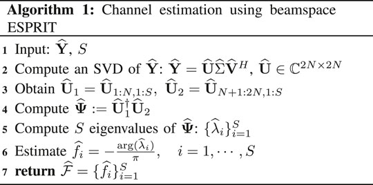
4 Review of Beamspace ESPRIT for mmWave Channel Estimation

In recent times, there has been a renewed interest in utilizing classical subspace-based techniques from array signal processing for mmWave channel estimation, due to similarities between the two measurement models at mmWave frequencies (Guo et al., 2017; Liao et al., 2017; Zhang and Haardt, 2017; Ma et al., 2020). An obvious advantage of these subspace-based algorithms is that they enable “gridless super-resolution” estimation of the AoAs that grid-based sparse techniques fail to achieve. Specifically, variants of subspace algorithms in the beamspace have been proposed that can produce high-resolution estimates of channel parameters even with a limited number of RF chains. In (Ma et al., 2020), Li et al. proposed a beamspace ESPRIT scheme which is applicable for any choice of beamformer, that satisfies some mild rank constraints. This approach requires only one antenna to be turned off at a time, and has several advantages such as a negligible drop in transmitted power and spatial coverage.

In this paper, we will analyze this variant of the beamspace ESPRIT algorithm. For ease of exposition, we will consider a flat-fading single carrier system, although extensions are possible. Our analysis will not require any specific assumptions on the distribution of noise, other than assuming it to be bounded. Unlike the prior asymptotic analysis in (Guanghan Xu et al., 1994; Mathews et al., 1996), we will not assume a large number of snapshots, or ignore higher-order perturbation terms (Roemer et al., 2014; Steinwandt et al., 2017). We first review the algorithm from (Ma et al., 2020) in the noiseless setting adapted to the flat-fading scenario.

The key idea behind the ESPRIT algorithm is exploiting the so-called shit invariance property, which refers to arrays with two identical subarrays that are separated by a common displacement. Let ${\mathbf{A}}_1(\mathcal{F})$, and ${\mathbf{A}}_2(\mathcal{F})$ denote two subarrays of $\mathbf{A}(\mathcal{F})$ comprising of the first and last M − 1 antenna elements. The array $\mathbf{A}(\mathcal{F})$ exhibits shit invariance property since

where $\mathbf{\Phi }(\mathcal{F})=\text{diag}(e^{-j\pi f_1},\dots ,e^{-j\pi f_S})$. One way to realize such subarrays and the corresponding shift invariance is by successively turning off the first and the last antennas. In (Ma et al., 2020), a two-stage approach was utilized to obtain this invariance structure. In the first stage, the Mth antenna is turned off, which corresponds to a beamforming matrix ${\tilde{\mathbf{W}}}_1≔{[{\mathbf{W}}^H,{\mathbf{0}}_N]}^H\in {\mathbb{C}}^{M\times N}$. In the second stage, the first antenna is turned off, yielding a beamforming matrix ${\tilde{\mathbf{W}}}_2≔{[{\mathbf{0}}_N,{\mathbf{W}}^H]}^H\in {\mathbb{C}}^{M\times N}$. Here $\mathbf{W}\in {\mathbb{C}}^{(M-1)\times N}$ is an analog beamforming matrix which satisfies the following rank condition:

A necessary condition for Eq. 6 is N ≥ S. Let ${\tilde{\mathbf{Y}}}_1={\tilde{\mathbf{W}}}_1^H{\mathbf{A}}_M(\mathcal{F})\mathbf{X}$, and ${\tilde{\mathbf{Y}}}_2={\tilde{\mathbf{W}}}_2^H{\mathbf{A}}_M(\mathcal{F})\mathbf{X}$ be the beamspace measurements acquired using this scheme. We define an augmented observation $\tilde{\mathbf{Y}}$ as

Define

where $\mathbf{\Phi }(\mathcal{F})=\text{diag}(e^{-j\pi f_1},\dots ,e^{-j\pi f_S})$, and ${\mathbf{A}}_1(\mathcal{F})\in {\mathbb{C}}^{(M-1)\times S}$, ${\mathbf{A}}_2(\mathcal{F})\in {\mathbb{C}}^{(M-1)\times S}$ comprise of the first and last M − 1 rows of ${\mathbf{A}}_M(\mathcal{F})$, respectively. For the rest of paper, we suppress the dependence on $\mathcal{F}$ and simply use A₁, A₂, Φ. Thus, Eq. 7 can be represented as

Note that under the assumption Eq. 6, we have rank(B) = S. We further assume that X has full row rank which together with rank(B) = S implies that $\text{rank}(\tilde{\mathbf{Y}})=S$. Let ${\mathbf{U}}_y{\mathbf{\Sigma }}_y{\mathbf{V}}_y^H=\tilde{\mathbf{Y}}$ be a reduced singular value decomposition (SVD) of $\tilde{\mathbf{Y}}\in {\mathbb{C}}^{2N}$, where ${\mathbf{U}}_y\in {\mathbb{C}}^{2N\times S},{\mathbf{\Sigma }}_y\in {\mathbb{C}}^{S\times S},{\mathbf{V}}_y\in {\mathbb{C}}^{T\times S}$. Since rank(B) = S, its columns form a basis for $\mathcal{R}(\tilde{\mathbf{Y}})$⁴ (which coincides with $\mathcal{R}({\mathbf{U}}_y)$). Thus, there exists an invertible matrix $\mathbf{P}\in {\mathbb{C}}^{S\times S}$ which provides a mapping between these two bases for $\mathcal{R}(\tilde{\mathbf{Y}})$,

Let U₁, and U₂ be two submatrices of U_y, comprising of its first and last N rows, respectively. Then,

Notice that $\mathbf{\Psi }≔{\mathbf{U}}_1^{†}{\mathbf{U}}_2={\mathbf{P}}^{-1}\mathbf{\Phi }\mathbf{P}$.⁵ Since Ψ is diagonalized by P, we can determine the AoAs (contained in Φ) from the S eigenvalues ${\{{\lambda }_i\}}_{i=1}^S$ of Ψ as follows:

where arg(λ) ∈ [−π, π) denotes the phase of the complex number λ.

The noiseless beamspace ESPRIT described above can be directly extended to a noisy setting. Consider the following noisy version of the measurement model introduced in Eq. 7:

where $\mathbf{N}\in {\mathbb{C}}^{M\times T}$ denotes the additive noise. The noisy version of the beamspace ESPRIT algorithm follows on similar lines as its noiseless version, and is summarized in Algorithm 1.

5 Performance Analysis of Beamspace ESPRIT

We will analyze the performance of the noisy beamspace ESPRIT algorithm. Our analysis extends the recent results from (Li et al., 2020) (for single-snapshot ESPRIT), to beamspace and multi-snapshot scenarios. Our error bounds will explicitly capture the role of the beamforming matrix W, and provide insights into how the error is shaped by the interaction between the AOA ($\mathcal{F}$) and beamforming matrix (W). We will use this characterization to develop new criteria for robust beamformer design in Section 2.

We first define some key quantities and metrics. The wrap around distance between two spatial frequencies f_i, f_j ∈ [0, 1] over the unit interval is defined as:

Our error metric will be the “matching distance” between the estimated $\widehat{\mathcal{F}}$ and ground truth $\mathcal{F}$, defined as:

where ψ is taken over all permutations of {1, 2, … , S}. Matching distance between the eigenvalues of $\widehat{\mathbf{\Psi }}$ and Ψ is similarly defined as

We will use the notation σ_k(Q) to denote the kth largest singular value of a matrix Q.

The following theorem provides an upper bound on the matching distance error between the true AoAs $\mathcal{F}$ and its estimate $\widehat{\mathcal{F}}$ obtained from beamspace ESPRIT:

Theorem 1. Consider the noisy measurement model Eq. 14. Let $\widehat{\mathcal{F}}$ be the estimated frequencies obtained from the beamspace ESPRIT algorithm (Algorithm 1). Assume that rank(BX) = S. If the noise level is moderately small such that

then the matching distance error between $\widehat{\mathcal{F}}$ and $\mathcal{F}$ is bounded as

Here C is a universal constant, and ${\mathbf{U}}_1\in {\mathbb{C}}^{N\times S}$ is defined in Eq. 11.

Proof. The proof follows by combining Lemma 6 and 8 of Appendix. See Supplementary Appendix for the details.

Remark 1. When S = 1, the bound Eq. 18 can be simplified to

where C′ is a constant. The quantity ‖W^Ha (f₁)‖₂ controls the error bound and represents the beamformer response to the spatial frequency f₁ (direction θ₁). Note that a simple scaling of the beamforming matrix W cannot improve performance since it boosts both the noise and signal components. For N = 1, ‖W^Ha (f₁)‖₂ = |w^Ha (f₁)| represents the beamforming gain in direction θ₁. Of course, if we knew f₁, we would choose w = a (f₁) to maximize |w^Ha (f₁)|. In that case, $\Vert {\mathbf{W}}^H\mathbf{a}(f_1){\Vert }_2/\Vert \mathbf{W}{\Vert }_2=\sqrt{M}$, and the error will scale as $1/\sqrt{M}$. However, during channel sensing, f₁ is unknown and w needs to be designed to ensure that a certain beamforming gain is achieved over a target sector of interest. Such a design will also decrease the error bound uniformly over that region. In the next section, this will be the basis for beamformer design.

6 Analog Beamformer Design for Maximizing the Minimum Gain

6.1 Review of Existing Beamformer Design Approaches

As explained earlier, the choice of the beamformer is implicitly tied to $\mathcal{F}$. However, prior to channel estimation, the AoAs ($\mathcal{F}$) of the multipaths are unknown, and it becomes impossible to beamform along these directions. As an alternative, in order to ensure beamforming gain over all possible multipath angles, it is common to assume that the AoAs belong to a sector of interest (Alkhateeb et al., 2014b; Ma et al., 2020). Let $\mathbb{T}:[f_{\text{min}},f_{\text{max}}]$ be a spatial sector of interest, and suppose we have prior knowledge that the AoAs $f_i\in \mathbb{T}$. We will now review beamformer designs that utilize this prior information to enhance the performance of channel estimation algorithms when AoAs are within this sector of interest (Chen et al., 2019; Ma et al., 2020). The most widely used criterion for designing a hybrid beamformer for mmWave channel sensing is to ensure (i) a constant beamforming gain over the sector of interest, and (ii) zero gain outside the region $\mathbb{T}$, i.e.,

where g is the desired gain. The criterion Eq. 20 represents an ideal brick-wall filter, and it cannot be realized in practice. A common approach is to ensure the desired gain g only on a finite grid of discretized frequencies (Chen et al., 2019; Alkhateeb et al., 2014b; Ma et al., 2020). Specifically, Let ${\mathbf{A}}_g=[{\mathbf{a}}_{{\tilde{f}}_1},{\mathbf{a}}_{{\tilde{f}}_2},\dots ,{\mathbf{a}}_{{\tilde{f}}_{N_g}}]\in {\mathbb{C}}^{M\times N_g}$ be a dictionary of steering vectors $\mathbf{a}({\tilde{f}}_k)$ corresponding to N_g grid points with

Suppose k₁ and k₂ are respectively the smallest and largest integers such that ${\tilde{f}}_{k_1},{\tilde{f}}_{k_2}\in \mathbb{T}$. We introduce a vector $\mathbf{g}\in {\mathbb{C}}^{N_g}$:

which enforces the gain constraints Eq. 20 at the discretized directions ${\tilde{f}}_k$. Note that a phase term ϕ_i is introduced to the response to provide additional flexibility of design. The first step towards designing the desired beamformer w involves estimating an ideal beamformer (v*) design by solving the following least square problem (Alkhateeb et al., 2014b; Chen and Qi, 2018; Chen et al., 2019; Ma et al., 2020):

Typically, the grid is chosen to satisfy N_g > M, which implies that rank (A_g) = M, and a closed form solution for the design is given by ${\mathbf{v}}^{*}={({\mathbf{A}}_g{\mathbf{A}}_g^H)}^{-1}{\mathbf{A}}_g\mathbf{g}=1/M{\mathbf{A}}_g\mathbf{g}$. The beamformers are normalized to obtain v₀ = v*/‖v*‖₂. In a typical hybrid mmWave system, the beamformer v₀ is realized by a hybrid structure where ${\mathbf{W}}_{\text{RF}}\in {\mathbb{C}}^{M\times N}$ is an RF (analog) beamformer implemented using phase shifters, i.e.

and a digital beamformer ${\mathbf{w}}_{\text{BB}}\in {\mathbb{C}}^{N\times 1}$. Therefore, the second stage of the beamformer design involves approximating the ideal design v₀ under these additional constraints imposed by the hardware, resulting in the following optimization problem (Alkhateeb et al., 2014b; Chen et al., 2019)

Several algorithms have been proposed to approximately solve Eq. 22 based on Orthogonal Matching Pursuit (Ayach et al., 2014; Alkhateeb et al., 2014b), alternating minimization (Yu et al., 2016; Chen et al., 2019), and fast search based techniques (Chen and Qi, 2018; Chen et al., 2019) using suitable initialization schemes.

Recently, instead of enforcing the constraint Eq. 20, the authors in (Ma et al., 2020) consider parametric beamformers of the following form, parameterized by $a\in \mathbb{R}$

where each beamformer is responsible for a partition of $\mathbb{T}$ determined by ${\{f_{(n)}\}}_{n=0}^N\in \mathbb{T}$. They propose to maximize the following ratio as a function of the parameter a

The numerator of S(a) represents the power concentrated in the sector of interest $\mathbb{T}$, and the denominator represents the total power. This criterion is maximized by performing a grid-based search over a after simplifying the ratio Eq. 24. One drawback of both of the aforementioned beamforming strategies is that the design is not guaranteed to ensure a constant gain of g even on the grid points. More importantly, the beamforming gain can drop below the desired level (g) at several regions in $\mathbb{T}$. There is no analytical characterization of how small the gain can become in these regions. This can lead to significant performance degradation of beamspace channel sensing techniques, especially if the multipath directions are aligned with the above regions where gain is small. In order to overcome these drawbacks, in the next section, we will propose a new “max-min” criterion for beamformer design to boost the minimum beamforming gain over $\mathbb{T}$. Such a criterion will allow more robust channel estimation uniformly over $\mathbb{T}$.

6.2 Beamformer Design Strategy

We motivate our approach for beamformer design by focusing on the quantity σ_S(W^HA), and relate it to the beamforming gain. It can be seen from Eq. 18 that larger the value of σ_S(W^HA), smaller the error of beamspace ESPRIT. Hence, one can aim to design W that maximizes σ_S(W^HA). But such a W will depend on $\mathbf{A}(\mathcal{F})$, and we do not know the AoA’s $\mathcal{F}$ to begin with. In many cases however, we can assume that the AoA belong to a region/sector of interest given by $\mathbb{T}≔[f_{\text{min}},f_{\text{max}}]$. In other words

In this case, we wish to ensure that ${\sigma }_S({\mathbf{W}}^H\mathbf{A}(\mathcal{F}))$ stays uniformly large over the entire set $\mathbb{T}$. Let α_W be the smallest value that ${\sigma }_S({\mathbf{W}}^H\mathbf{A}(\mathcal{F}))$ can assume over $\mathbb{T}$, i.e.,

We wish to design W in order to maximize α_W (under constant modulus constraints on W), which leads to the following problem:

This problem belongs to the family of non-convex max-min optimization problems, and it is challenging to solve it for the most general setting. In the next section, we focus on providing the solution of such an optimization problem for the scenario when there is a single source S = 1, single RF chain N = 1, and contrast the distinctions between the proposed criteria to the existing beamformer designs reviewed in Section 1.

6.3 Optimal Solution for Single Source and Single RF Chain

We consider the single path scenario (S = 1) where the channel is given by h_t = α_ta(f). This model has been widely used in the mmWave communication literature where the path losses are high and the channel is assumed to have only a single Line of Sight (LOS) path that is dominant (Alkhateeb et al., 2014b; Chiu et al., 2019). Our goal will be to optimize the design of a single RF chain (N = 1), which is again motivated by typical hybrid mmWave hardware systems that are equipped with large antenna arrays but often just 1 RF chain (Roh et al., 2014). For S = 1, N = 1, it can be verified that ${\sigma }_S({\mathbf{W}}^H\mathbf{A}(\mathcal{F}))={\sigma }_1({\mathbf{w}}^H\mathbf{a}(f))=|{\mathbf{w}}^H\mathbf{a}(f)|$. We first develop a framework for designing w that is optimized to maximize the minimum gain over the entire sector of interest. Specifically, this yields the following max-min problem:

Notice that Eq. 26 aims to maximize the minimum (or worst case) gain of the beamformer over the sector $\mathbb{T}$. At this point, we will like to distinguish the criterion Eq. 26 from those discussed in Section 1. Although the quantity of interest is w^Ha(f) in both cases, the design criteria reviewed in Section 1 are fundamentally different from Eq. 26. Firstly, the approaches in (Alkhateeb et al., 2014b; Chen and Qi, 2018; Chen et al., 2019) solve a grid-based least square loss Eq. 21, and therefore the obtained design is not guaranteed to ensure constant gain g even on the grid points. Indeed, there could be an adversarial multipath angle $f_0\in \mathbb{T}$ where the observed gain is lower:

In contrast, the criterion Eq. 26 can uniformly guarantee beamforming gain of at least ${\eta }_{\mathbb{T}}^{\star }$ in the entire sector $\mathbb{T}$. This is illustrated in Figure 1 where we plot the gain of two different beamformers against the max-min design over the sector of interest $\mathbb{T}=[\mathrm{0,0.2}]$. As can be seen, the gain for “power-ratio” (Ma et al., 2020) and “constant gain” designs (Chen et al., 2019) both significantly fall below the desired level along several directions in the sector $\mathbb{T}$, whereas for the max-min design the smallest (worst case) gain is larger than the other designs.

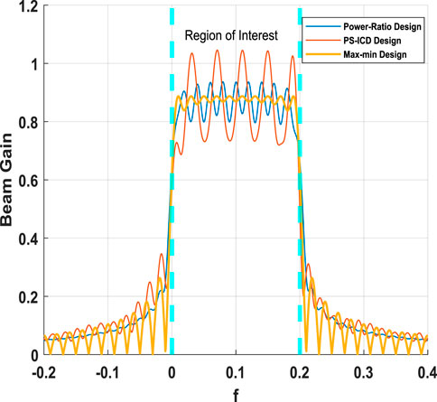
FIGURE 1. Comparison of beam patterns of two different beamformer designs against the max-min design. Here N = 10, M = 128, $\mathbb{T}=[\mathrm{0,0.2}]$.

Solving Eq. 26 over the set of all unimodular w can be a challenging problem, and it can be difficult to quantify and analyze the optimal solution. To make Eq. 26 tractable so that we can obtain a closed form solution with “quantifiable” minimum beamforming gain over the entire sector $\mathbb{T}$, we propose to choose w from a parametric class ${\mathcal{W}}_{\mathbb{T}}$ of beamformers, which already obey the unimodular constraints. We define ${\mathcal{W}}_{\mathbb{T}}$ as follows. Given a “center frequency” $f_c\in \mathbb{T}$, and an integer m_a, 1 ≤ m_a ≤ M, define $\mathbf{b}(f_c,m_a)\in {\mathbb{C}}^M$ as

Hence, b (f_c, m_a) represents a DFT beamformer with m_a active antennas and whose pass band is centered at f_c. Let $m_r≔\min \{\frac{4}{f_{\text{max}}-f_{\text{min}}},M\}$. Given an integer m_a satisfying 1 ≤ m_a ≤ m_r, we define ${\mathcal{C}}_{m_a,\mathbb{T}}\subset {\mathbb{C}}^M$ as the set of all DFT beamformers with m_a active antennas, generated by varying the center frequency f_c over the interval $[f_{\text{max}}-\frac{2}{m_a},f_{\text{min}}+\frac{2}{m_a}]$:

All beamformers in ${\mathcal{C}}_{m_a,\mathbb{T}}$ therefore have the same beamwidth determined by m_a with the flexibility of shifting the beam centers to any location f_c such that the desired coverage region $\mathbb{T}$ remains in the main lobe of the beam, i.e., $\mathbb{T}\subset [f_c-\frac{2}{m_a},f_c+\frac{2}{m_a}]$. Finally, we define the set ${\mathcal{W}}_{\mathbb{T}}$ that comprises of DFT beamformers of all possible mainlobe widths, i.e.,

Using this class ${\mathcal{W}}_{\mathbb{T}}$, we propose to solve

Notice that the class of beamformers ${\mathcal{W}}_{\mathbb{T}}$ is quite broad, consisting of multi-resolution beams of varying beam widths (determined by m_a), and for each resolution/beamwidth the permissible beams are shifted copies of each other. Such beamformers have two fold-advantages (i) they inherently satisfy the desired constant modulus constraint for hardware implementation using phase shifters and switches, and (ii) they are amenable to theoretical analysis due to the parametric structure. A key distinction compared to the designs described in Section 1 is that we are only considering purely RF or analog beamformers, without any baseband processing. As will be shown in the simulations, with the same budget of RF chains, this max-min design strategy yields superior performance compared to the hybrid designs, especially for adversarial multipath configurations.

The max-min design criterion involves a natural trade-off between gain and coverage. As shown in Figure 2, when m_a is large the resulting beams are sharper and can offer higher gains. Despite their higher gain, their coverage is limited owing to the narrow main lobes. Since our goal is to ensure a certain minimum gain uniformly across the entire sector $\mathbb{T}$, we must design the beam centers and select the widths appropriately to satisfy this objective. The parametric structure of ${\mathcal{W}}_{\mathbb{T}}$ allows us to obtain the following expression for the beamforming gain for w = b (f_c, m_a):

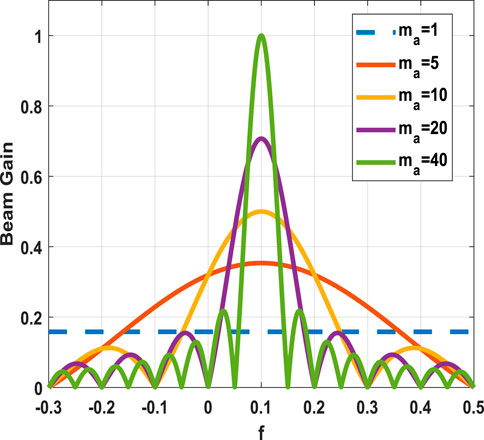
FIGURE 2. Effect of the number of active antennas on the realizable beam patterns in ${\mathcal{W}}_{\mathbb{T}}$ with a single RF chain (N = 1, M = 40).

Owing to the structure of ${\mathcal{W}}_{\mathbb{T}}$, searching for the optimum w reduces to finding the optimum center f_c and active antennas m_a that jointly maximize the minimum gain over the entire sector of interest $\mathbb{T}$. Theorem 2 provides the optimal choice of this design.

Theorem 2. Let $\mathbb{T}=[f_{\text{min}},f_{\text{max}}]\in [\mathrm{0,1}]$, Δ_f≔f_max − f_min. Given the class of beamformers ${\mathcal{W}}_{\mathbb{T}}$ defined in Eq. 27, the optimal value of Eq. 28 is given by

The optimal value is attained by the beamformer $\mathbf{b}(f_c^{*},m_a^{*})\in {\mathcal{W}}_{\mathbb{T}}$ where

where notation [x] refers to the closest integer to x.

Proof. The problem Eq. 28 is equivalent to the following problem

where ${\mathcal{D}}_{M,\mathbb{T}}$ denotes the set of (f_c, m_a) pairs such that $\mathbf{b}(f_c,m_a)\in {\mathcal{W}}_{\mathbb{T}}$:

Fix m_a. Define $g_{(f_c,m_a)}:\mathbb{T}\to {\mathbb{R}}_{+}$ as:

The function $g_{(f_c,m_a)}(f)$ is symmetric around f_c, and is monotonically increasing for f ∈ [f_c − 2/m_a, f_c] and monotonically decreasing for f ∈ [f_c, f_c + 2/m_a]. Since $(f_c,m_a)\in {\mathcal{D}}_{M,\mathbb{T}}$, we have $\mathbb{T}\subset [f_c-2/m_a,f_c+2/m_a]$ for all $(f_c,m_a)\in {\mathcal{D}}_{M,\mathbb{T}}$. Therefore, it holds that

We first consider

Based on the definition of $g_{(f_c,m_a)}(f)$, for all $(f_c,m_a)\in {\mathcal{D}}_{M,\mathbb{T}}$ we have

Further the fact $(f_c,m_a)\in {\mathcal{D}}_{M,\mathbb{T}}$ along with Eq. 34 implies that

Thus

Using Eqs 33–35, 37 we have

where the inequality (a) follows from the monotonically increasing behavior of g over the interval [f_c − 2/m_a, f_c], and Eq. 36 which implies f_min ∈ [f_c − 2/m_a, f_c]. The inequality (b) follows from the fact that $f_{\min }\in \mathbb{T}$. Hence, we get

Using a similar argument we can show that Eq. 38 also holds when f_c ≤ f_mid.Notice Eq. 32 implies that

Therefore, it can be easily verified that the maximum value of $g_{(f_{\text{mid}},m_a)}(f_{\text{min}})$ over all $(f_c=f_{\text{mid}},m_a)\in {\mathcal{D}}_{M,\mathbb{T}}$ pairs is given as

which will be attained at

Optimality of $(f_{mid},m_a^{*})$ implies that for all $(f_c=f_{mid},m_a)\in {\mathcal{D}}_{M,\mathbb{T}}$ we have,

Hence as the result of Eq. 38, and Eq. 43, for any $(f_c,m_a)\in {\mathcal{D}}_{M,\mathbb{T}}$ we have

which completes the proof.

6.4 A Sub-band Splitting Design for Multiple RF Chains

We now develop a heuristic for N > 1 RF chains that utilizes the optimal design from Theorem 2. When N > 1, let $\mathbf{W}=[{\mathbf{w}}_1,{\mathbf{w}}_2,\dots ,{\mathbf{w}}_N]\in {\mathbb{C}}^{M\times N}$ be the analog beamforming matrix. In this case, σ_S(W^Ha(f)) assumes the form

Similar to our prior objective, we now wish to ensure the minimum value of $\Vert {\mathbf{W}}^H\mathbf{a}(f){\Vert }_2^2$ is maximized:

Instead of exactly solving Eq. 44, we will use our design for 1 RF chain to develop a subband splitting approach for designing w₁, w₂, … , w_N. In particular, given the interval $\mathbb{T}$ and a budget of N RF-chains, we partition $\mathbb{T}$ into N subbands,

where ${\mathbb{T}}_k≔[f_{\text{min}}+({\mathrm{\Delta }}_f)\frac{k-1}{N},f_{\text{min}}+({\mathrm{\Delta }}_f)\frac{k}{N}]$ represents the kth partition or subband of the sector. Such a subband design was also considered in (Ma et al., 2020), but the criterion was different. In particular, in (Ma et al., 2020), each beamformer is responsible for maximizing the ratio Eq. 24 in the subband. Instead of maximizing the power-ratio, we propose to maximize the worst-case gain within each subband, which will prove to be more robust, especially for adversarial settings. We solve N different optimization problems to find w_i, i = 1, 2, … , N as follows

As a result of the partition (Stewart, 1990), we can adopt the optimal design obtained from Theorem 2 for each of the N problems in (Hansen, 1987). This approach greedily designs the columns of the matrix W such that the kth beamformer w_k maximizes the minimum gain over ${\mathbb{T}}_k$. Let $f_c^{(k)}$ and $m_a^{(k)}$ be the center and number of active antenna for the optimum w_k that solves Eq. 46. Then, Theorem 2 dictates

This design follows from Theorem 2, where each of the N intervals ${\{{\mathbb{T}}_k\}}_{k=1}^N$ are of length Δ_f/N, hence the optimal value of $m_a^{(k)}$ is given by Eq. 30. In this case, we can obtain a lower bound on $\Vert {\mathbf{W}}^H\mathbf{a}(f){\Vert }_2^2$ by using the gain characterization from Theorem 2.

An example of this sub-band max-min design scheme is illustrated in Figure 3, where the sector of interest $\mathbb{T}=[\mathrm{0,0.5}]$ is partitioned into 5 subbands (partitions are shown using the dotted lines). Each of the available 5 RF chains maximize the beamforming gain in each subband. The solid line indicates the overall gain in the sector of interest showing reduced gain drop over $\mathbb{T}$.

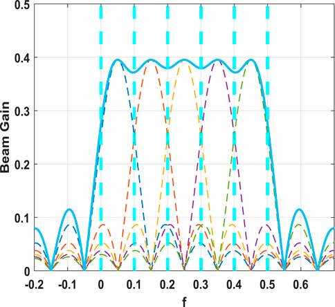
FIGURE 3. Subband splitting approach for designing N = 5 beamfomers by partitioning the region of interest into N = 5 subbands and choosing the optimal beamformer within each subband. A single RF chain is responsible for maximizing the minimum gain in each subband/partition.

7 Numerical Results

In this section, we experimentally validate our analysis of beamspace ESPRIT (in Theorem 1), and also evaluate the performance of the max-min beamformer proposed in Section 2.

In the first experiment, we study the effect of varying the number (M) of antennas on the matching distance error. We fix the AOAs of the channel paths to be $\mathcal{F}=\{0.21,0.29,0.36,0.38\}$, which belong to the region of interest $\mathbb{T}=[0.2,0.4]$. For each M, the channel gains X are normalized to satisfy ‖X‖₂ = 1. The received signal in Eq. 4 is corrupted by bounded random noise, normalized to satisfy ‖N‖₂ = ϵ. We keep X fixed and only the noise is randomly generated during the Monte Carlo experiments. We compute the average matching distance error of beamspace ESPRIT for this channel configuration averaged over L = 500 different noise realizations. In Figure 4, we plot the average matching distance error of the beamspace ESPRIT algorithm using the max-min beamformer proposed in Section 2. Although the design was proposed for S = 1, it can be deployed for channels with S > 1 multipath components as well. We vary the number of antennas from M = 32 to M = 128 for two different noise levels ϵ = 0.1, 0.5. From Theorem 1, for a fixed channel configuration (fixed S, and $\mathcal{F}$), the matching distance error bound is proportional to β_M(W, N), given by

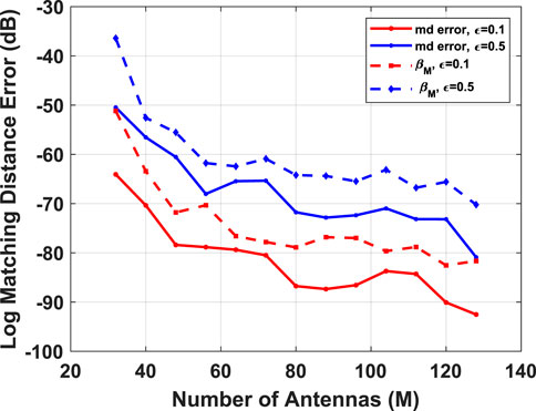
FIGURE 4. Comparative study of matching distance error as a function of the number of antennas M, using the max-min beamforming scheme for a multipath channel with S = 4 paths, N = 20 RF chains, T = 50 Snapshots. The dotted lines illustrate the trend predicted by the bounds in Theorem 1.

In order to validate the trend predicted by our theoretical result, we overlay the average β_M(W, N) (averaged over the noise realizations), scaled by a factor of 10^–3. As shown in Figure 4, the average matching distance error follows the trend predicted by the bound in Theorem 1. As expected, both the empirical error and the trend based on β_M(W, N) increase with ϵ. The fluctuations in error (which are also consistent with the fluctuations in the bound) can be attributed to the fact that as we vary M, the gain of the beamformers at the (fixed) AoAs also fluctuate.

We now compare the proposed max-min beamformer against three other beamformer design strategies (Li et al., 2020; Chen et al., 2019) which were reviewed in Section 1. In all of the following experiments, we choose $\mathbb{T}=[\mathrm{0,0.2}]$ as our region of interest. In all figures, “Power-Ratio” refers to the beamformer designed using Eq. 23 (Li et al., 2020), “PS-ICD” refers to the design in (Chen et al., 2019) which approximates the solution of Eq. 21 using phase shifters, and “DFT” refers to a sub-selection of the columns of a DFT matrix (according to the region of interest and number of available RF chains). “Max-Min design” denotes the beamformer described in Section 2, where we partition the region of interest $\mathbb{T}$ and construct the optimal beamformers corresponding to each region.

We first generate a single LOS path with $\mathcal{F}=\{0.18\}\in \mathbb{T}=[\mathrm{0,0.2}]$, and a fixed channel gain matrix X satisfying ‖X‖₂ = M. Similar to the previous setting, we consider bounded noise with ‖N‖₂ = ϵM to ensure that the ratio ‖X‖₂/‖N‖₂ is fixed. In Figure 5, we plot the average matching distance error for three different beamformers, and overlay the average trend predicted by β_M(W, N). The empirical average matching distance error exhibits a similar trend as predicted by β_M(W, N). The performance gap observed between the bounds is also reflected in the actual matching distance error, hence, illustrating the effectiveness of the proposed beamformer design by leveraging the error analysis.

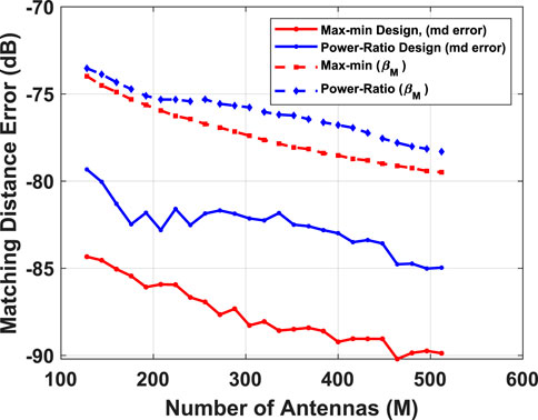
FIGURE 5. Comparative study of matching distance error as a function of the number of antennas M, using the max-min and power ratio beamforming schemes for a LOS channel with S = 1 path along $\mathcal{F}=[0.18]$, N = 10 RF chains, T = 5 snapshots, and noise level ϵ = 0.5. The dotted lines illustrate the trend predicted by the bounds in Theorem 1.

In Figures 6–12, we assume that the path gains are i. i.d random variables distributed as $x_{s,t}\sim \mathcal{N}C(0,{\sigma }_x)$. Furthermore, the noise are assumed to be i. i.d random variables distributed as $n_{m,t}\sim \mathcal{N}C(0,{\sigma }_n)$ and independent from the channel gains. We define SNR as

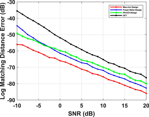
FIGURE 6. Comparison of performance of max-min beamformer against power-ratio, PS-ICD and DFT beamformers as a function of SNR, with channel path directions given by $\mathcal{F}=[0.18]$. Each beamformer design is realized with N = 5 RF chains where M = 64.

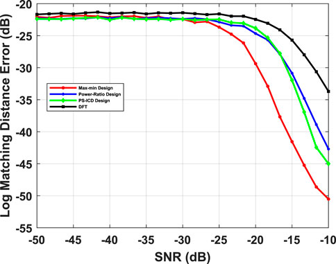
FIGURE 7. Comparison of channel estimation performance of max-min beamformer against power-ratio, PS-ICD and DFT beamformers in the SNR regime of −50 dB to −10 dB, with channel path directions given by $\mathcal{F}=[0.18]$. Each beamformer design is realized with N = 5 RF chains where M = 64.

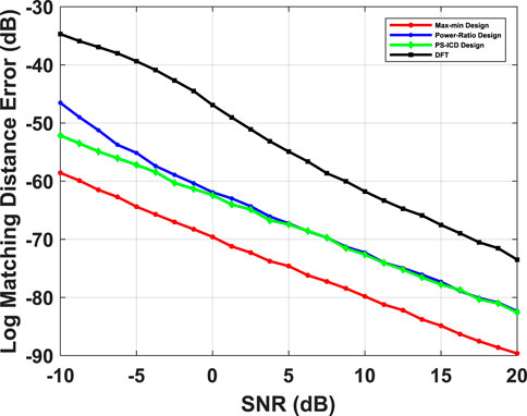
FIGURE 8. Comparison of performance of max-min beamformer against power-ratio, PS-ICD and DFT beamformers as a function of SNR, with channel path directions given by $\mathcal{F}=[0.02,0.1,0.16,0.18]$. Each beamformer design is realized with N = 10 RF chains where M = 128.

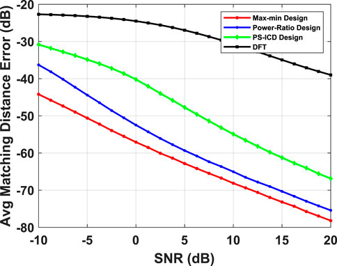
FIGURE 9. Comparison of beamspace channel estimation performance for a LOS channel with S = 1 path, M = 64 antennas, N = 5 RF chains as a function of SNR. The plot shows the matching distance error averaged over K = 100 different channel realizations by varying one of the AOAs uniformly on a grid in the region of interest.

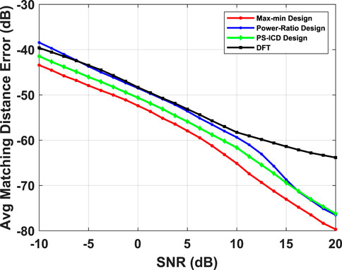
FIGURE 10. Comparison of beamspace channel estimation performance for a multipath channel with S = 4 path, M = 128 antennas, N = 10 RF chains as a function of SNR. The plot shows the matching distance error averaged over K = 100 different channel realizations by varying the one AOA uniformly on a grid in the region of interest while three other AOAs are fixed at [0.02, 0.1, 0.18].

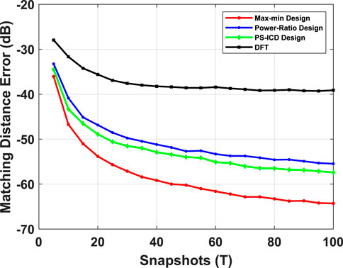
FIGURE 11. Matching distance error vs. the number of snapshots for max-min beamformer and power-ratio, PS-ICD and DFT beamformers. The channel path directions are given by $\mathcal{F}=[0.02,0.1,0.16,0.18]$. Each beamformer design is realized with N = 10 RF chains where M = 128.

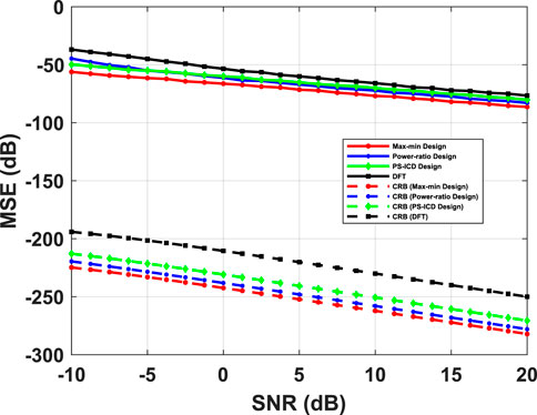
FIGURE 12. Comparative study of MSE and Cramér-Rao Bound (CRB) as a function of SNR, using the max-min and power ratio beamforming schemes for a LOS channel with S = 1 path along $\mathcal{F}=[0.18]$, N = 5 RF chains, M = 64 Antennas, T = 100 snapshots. The dotted lines denote beamspace CRB.

In Figures 6–8, we compare the average Matching Distance error of beamspace ESPRIT as a function of SNR, using different beamformers. In Figures 6, 7, the channel is assumed to have a single LOS path, with M = 64 antennas, N = 5 RF chains, and T = 50 snapshots. In Figure 8, we consider a multi-path channel with S = 4 paths, M = 128 antennas, N = 10 RF chains, and T = 50 temporal snapshots. We considered a specific channel configuration where the AoAs are chosen from the set $\mathcal{F}=\{0.02,0.1,0.16,0.18\}$. As can be observed, the max-min design outperforms other schemes uniformly over the entire range of SNR, maintaining a gap in error of about 10 dB. In Figure 7, we further show how the performance of all the beamformers degrade when the SNR becomes very small. In such a low SNR regime, the matching distance error of one channel path converges to half of the length of the region of interest, i. e 20 log ₁₀ (0.1) = −20 dB.

In the next experiment, we investigate the performance of max-min beamformer with respect to different path directions over the region of interest. In order to do so, we choose the path angles from a uniform grid of size K = 100 over the region of interest $\mathbb{T}$, and plot the average matching distance error (Avg-md) over all possible channel configurations. For a single path LOS channel, let ${\mathcal{F}}_k=\left\{\frac{0.2(k-1)}{K}\right\}$ be the AoA direction while ${\widehat{\mathcal{F}}}_{k,l}$ refers to the estimate of ${\mathcal{F}}_k$ for the lth realization. The Avg-md is given as follows

In Figure 9 we plot the Avg-md as a function of SNR, under a similar setting as Figure 6. In Figure 10, we repeat this for a multi-path channel, where three path directions are fixed, and the AoA of the fourth path is varied over $\mathbb{T}$, i. e, ${\mathcal{F}}_k=\left\{0.02,0.1,0.18,\frac{0.2(k-1)}{K}\right\}$. The superior performance of the Max-Min beamformer can be attributed to the fact that its minimum gain over $\mathbb{T}$ is always larger than that of the other beamformers.

Owing to a higher “worst-case gain” over the region of interest, max-min beamformers enable a more robust channel estimation in face of certain (adversarial) channel configurations/multipath directions, compared to the other beamformers whose pass-band gain can drop significantly below the desired (constant) level for these directions, resulting in an overall degradation of the average error.

In Figure 11, we demonstrate the effect of the total number of temporal snapshots on the ESPRIT matching distance error for different beamforming schemes. In this experiment, we fix the SNR at −5 dB, and the other parameters are identical to those used in Figure 8. The plot shows that our schemes is effective even in the limited snapshot regime. Additionally, the gap between the performance of Min-Max design and the other beamformers steadily increases with the number of snapshots.

Finally, Figure 12 compares the MSE of beamspace ESPRIT against the beamspace Cramér-Rao Bound (CRB) for different beamformers (Van Trees, 2004), under a similar setting as Figure 6. As we can observe, the trend exhibited by the empirical MSE is consistent with the trend shown by the CRB, and the max-min beamformers exhibit a smaller CRB compared to other beamformers.

8 Conclusion

In this work, we have extended the analysis of single-snapshot ESPRIT for beamspace and multi-snapshot scenarios. Our analysis is non-asymptotic in the number of snapshots, and provides an upper bound on the matching distance error without requiring any specific distribution for the noise. The error analysis revealed the role of the beamformer design. Based on our theoretical analysis, we have proposed a novel max-min criterion for designing beamformers which ensures a minimum beamforming gain uniformly over a region of possible path directions. We have considered a family of multi-resolution beamformers which can be implemented with phase shifters, and proposed the optimal beamformers from this family with respect to the new max-min criteria. By conducting several numerical experiments, we have empirically established the superior performance of our designed beamformers compared to other beamformers. In future, an interesting question would be to extend the max-min design over a broader class of beamformers.

Data Availability Statement

The raw data supporting the conclusions of this article will be made available by the authors, without undue reservation.

Author Contributions

SS, PS, and PP developed the main conceptual idea and theoretical results presented in paper. SS, PS, and PP planned the experiments and numerical results presented in the manuscript. All authors contributed in writing the manuscript and approved the content of the submitted version.

Conflict of Interest

The authors declare that the research was conducted in the absence of any commercial or financial relationships that could be construed as a potential conflict of interest.

Publisher’s Note

All claims expressed in this article are solely those of the authors and do not necessarily represent those of their affiliated organizations, or those of the publisher, the editors and the reviewers. Any product that may be evaluated in this article, or claim that may be made by its manufacturer, is not guaranteed or endorsed by the publisher.

Supplementary Material

The Supplementary Material for this article can be found online at: https://www.frontiersin.org/articles/10.3389/frsip.2021.820617/full#supplementary-material

Footnotes

¹This work was supported in part by the Office of Naval Research under Grants ONR N00014-19-1-2256 and ONR N00014-19-1-2227, and in part by the National Science Foundation under Grant NSF CAREER ECCS 1700 506.

²The results can also be extended to channels that exhibit frequency selectivity by considering orthogonal frequency-division multiplexing (OFDM), where the channel vector at each subcarrier can be described by Eq. 1.

³For multi-user system, we can reduce the problem to single-user using orthogonal pilots.

⁴$\mathcal{R}(\tilde{\mathbf{Y}})$ denotes the range space of $\tilde{\mathbf{Y}}$.

⁵${\mathbf{U}}_1^{†}$ denotes the Moore-Penrose Pseudo-inverse of the rectangular matrix U₁.

References

A. Proof of Auxiliary Lemmas for Theorem 1

Our proof follows similar arguments as [1] with necessary modifications for beamspace and multi-snapshot scenario. For completeness, we provide all auxiliary lemmas used.

Preliminaries

Let S₁, S₂ be any orthonormal bases for $\mathcal{R}({\mathbf{U}}_y)$ and $\mathcal{R}({\widehat{\mathbf{U}}}_y)$, respectively. The principal (or canonical) angles between the subspaces $\mathcal{R}({\mathbf{U}}_y)$ and $\mathcal{R}({\widehat{\mathbf{U}}}_y)$ are defined as the $\mathbf{\Theta }({\mathbf{S}}_1,{\mathbf{S}}_2)≔{[{\omega }_1,{\omega }_2,\dots ,{\omega }_S]}^T$ where ω_k ∈ [0, π/2] satisfies:

References

Alkhateeb, A., El Ayach, O., Leus, G., and Heath, R. W. (2014). Channel Estimation and Hybrid Precoding for Millimeter Wave Cellular Systems. IEEE J. Sel. Top. Signal. Process. 8 (5), 831–846. doi:10.1109/jstsp.2014.2334278
Alkhateeb, A., and Heath, R. W. (2016). Frequency Selective Hybrid Precoding for Limited Feedback Millimeter Wave Systems. IEEE Trans. Commun. 64 (5), 1801–1818. doi:10.1109/tcomm.2016.2549517
Alkhateeb, A., Mo, J., Gonzalez-Prelcic, N., and Heath, R. W. (2014). Mimo Precoding and Combining Solutions for Millimeter-Wave Systems. IEEE Commun. Mag. 52 (12), 122–131. doi:10.1109/mcom.2014.6979963
Ayach, O. E., Rajagopal, S., Abu-Surra, S., Pi, Z., and Heath, R. W. (2014). Spatially Sparse Precoding in Millimeter Wave Mimo Systems. IEEE Trans. Wireless Commun. 13 (3), 1499–1513. doi:10.1109/twc.2014.011714.130846
Bai, T., and Heath, R. W. (2014). Coverage and Rate Analysis for Millimeter-Wave Cellular Networks. IEEE Trans. Wireless Commun. 14 (2), 1100–1114.
Bauer, F. L., and Fike, C. T. (1960). Norms and Exclusion Theorems. Numer. Math. 2 (1), 137–141. doi:10.1007/bf01386217
Bogale, T. E., Le, L. B., and Wang, X. (2015). Hybrid Analog-Digital Channel Estimation and Beamforming: Training-Throughput Tradeoff. IEEE Trans. Commun. 63 (12), 5235–5249. doi:10.1109/tcomm.2015.2495191
Chen, K., and Qi, C. (2018). “Beam Design with Quantized Phase Shifters for Millimeter Wave Massive Mimo,” in 2018 IEEE Global Communications Conference (GLOBECOM) (IEEE), 1–7. doi:10.1109/glocom.2018.8647641
Chen, K., Qi, C., and Li, G. Y. (2019). Two-step Codeword Design for Millimeter Wave Massive Mimo Systems with Quantized Phase Shifters. IEEE Trans. Signal Process. 68, 170–180.
Chiu, S.-E., Ronquillo, N., and Javidi, T. (2019). Active Learning and Csi Acquisition for Mmwave Initial Alignment. IEEE J. Select. Areas Commun. 37 (11), 2474–2489. doi:10.1109/jsac.2019.2933967
Gao, Z., Hu, C., Dai, L., and Wang, Z. (2016). Channel Estimation for Millimeter-Wave Massive Mimo with Hybrid Precoding over Frequency-Selective Fading Channels. IEEE Commun. Lett. 20 (6), 1259–1262. doi:10.1109/lcomm.2016.2555299
González-Coma, J. P., Rodriguez-Fernandez, J., González-Prelcic, N., Castedo, L., and Heath, R. W. (2018). Channel Estimation and Hybrid Precoding for Frequency Selective Multiuser Mmwave Mimo Systems. IEEE J. Sel. Top. Signal. Process. 12 (2), 353–367. doi:10.1109/jstsp.2018.2819130
Guanghan Xu, G., Silverstein, S. D., Roy, R. H., and Kailath, T. (1994). Beamspace Esprit. IEEE Trans. Signal. Process. 42 (2), 349–356. doi:10.1109/78.275607
Guo, Z., Wang, X., and Heng, W. (2017). Millimeter-wave Channel Estimation Based on 2-d Beamspace Music Method. IEEE Trans. Wireless Commun. 16 (8), 5384–5394. doi:10.1109/twc.2017.2710049
Haardt, M., and Nossek, J. A. (1995). Unitary Esprit: How to Obtain Increased Estimation Accuracy with a Reduced Computational burden. IEEE Trans. Signal. Process. 43 (5), 1232–1242. doi:10.1109/78.382406
Haghighatshoar, S., and Caire, G. (2016). Massive Mimo Channel Subspace Estimation from Low-Dimensional Projections. IEEE Trans. Signal Process. 65 (2), 303–318.
Han, S., I, C.-l., Xu, Z., and Rowell, C. (2015). Large-scale Antenna Systems with Hybrid Analog and Digital Beamforming for Millimeter Wave 5g. IEEE Commun. Mag. 53 (1), 186–194. doi:10.1109/mcom.2015.7010533
Hansen, P. C. (1987). The Truncatedsvd as a Method for Regularization. Bit 27 (4), 534–553. doi:10.1007/bf01937276
Hur, S., Kim, T., Love, D. J., Krogmeier, J. V., Thomas, T. A., and Ghosh, A. (2013). Millimeter Wave Beamforming for Wireless Backhaul and Access in Small Cell Networks. IEEE Trans. Commun. 61 (10), 4391–4403. doi:10.1109/tcomm.2013.090513.120848
Junyi Wang, J., Zhou Lan, Z., Chang-woo Pyo, C.-w., Baykas, T., Chin-sean Sum, C.-s., Rahman, M. A., et al. (2009). Beam Codebook Based Beamforming Protocol for Multi-Gbps Millimeter-Wave Wpan Systems. IEEE J. Select. Areas Commun. 27 (8), 1390–1399. doi:10.1109/jsac.2009.091009
Lee, J., Gil, G.-T., and Lee, Y. H. (2016). Channel Estimation via Orthogonal Matching Pursuit for Hybrid Mimo Systems in Millimeter Wave Communications. IEEE Trans. Commun. 64 (6), 2370–2386. doi:10.1109/tcomm.2016.2557791
Li, W., Liao, W., and Fannjiang, A. (2020). Super-resolution Limit of the Esprit Algorithm. IEEE Trans. Inform. Theor. 66 (7), 4593–4608. doi:10.1109/tit.2020.2974174
Liao, A., Gao, Z., Wu, Y., Wang, H., and Alouini, M.-S. (2017). 2d Unitary Esprit Based Super-resolution Channel Estimation for Millimeter-Wave Massive Mimo with Hybrid Precoding. IEEE Access 5, 24747–24757. doi:10.1109/access.2017.2768579
Ma, W., Qi, C., and Li, G. Y. (2020). High-resolution Channel Estimation for Frequency-Selective Mmwave Massive Mimo Systems. IEEE Trans. Wireless Commun. 19 (5), 3517–3529. doi:10.1109/twc.2020.2974728
Mathews, C. P., Haardt, M., and Zoltowski, M. D. (1996). Performance Analysis of Closed-form, Esprit Based 2-d Angle Estimator for Rectangular Arrays. IEEE Signal. Process. Lett. 3 (4), 124–126. doi:10.1109/97.489068
Méndez-Rial, R., Rusu, C., González-Prelcic, N., Alkhateeb, A., and Heath, R. W. (2016). Hybrid MIMO Architectures for Millimeter Wave Communications: Phase Shifters or Switches. Ieee Access 4, 247–267. doi:10.1109/access.2015.2514261
Park, S., Ali, A., González-Prelcic, N., and Heath, R. W. (2019). Spatial Channel Covariance Estimation for Hybrid Architectures Based on Tensor Decompositions. IEEE Trans. Wireless Commun. 19 (2), 1084–1097.
Park, S., and Heath, R. W. (2018). Spatial Channel Covariance Estimation for the Hybrid Mimo Architecture: A Compressive Sensing-Based Approach. IEEE Trans. Wireless Commun. 17 (12), 8047–8062. doi:10.1109/twc.2018.2873592
Raghavan, V., and Sayeed, A. M. (2010). Sublinear Capacity Scaling Laws for Sparse Mimo Channels. IEEE Trans. Inf. Theor. 57 (1), 345–364.
Rakhimov, D., Zhang, J., de Almeida, A., Nadeev, A., and Haardt, M. (2019). “Channel Estimation for Hybrid Multi-Carrier Mmwave Mimo Systems Using 3-d Unitary Tensor-Esprit in Dft Beamspace,” in 2019 53rd Asilomar Conference on Signals, Systems, and Computers (IEEE), 447–451. doi:10.1109/ieeeconf44664.2019.9048951
Rodríguez-Fernández, J., González-Prelcic, N., Venugopal, K., and Heath, R. W. (2018). Frequency-domain Compressive Channel Estimation for Frequency-Selective Hybrid Millimeter Wave Mimo Systems. IEEE Trans. Wireless Commun. 17 (5), 2946–2960. doi:10.1109/twc.2018.2804943
Roemer, F., Haardt, M., and Del Galdo, G. (2014). Analytical Performance Assessment of Multi-Dimensional Matrix-And Tensor-Based Esprit-type Algorithms. IEEE Trans. Signal Process. 62 (10), 2611–2625.
Roh, W., Seol, J.-Y., Park, J., Lee, B., Lee, J., Kim, Y., et al. (2014). Millimeter-wave Beamforming as an Enabling Technology for 5g Cellular Communications: Theoretical Feasibility and Prototype Results. IEEE Commun. Mag. 52 (2), 106–113. doi:10.1109/mcom.2014.6736750
Roy, R., and Kailath, T. (1989). Esprit-estimation of Signal Parameters via Rotational Invariance Techniques. IEEE Trans. Acoust. Speech, Signal. Process. 37 (7), 984–995. doi:10.1109/29.32276
Sarangi, P., Shahsavari, S., and Pal, P. (2020). “Robust Doa and Subspace Estimation for Hybrid Channel Sensing,” in 2020 54th Asilomar Conference on Signals, Systems, and Computers (IEEE), 236–240. doi:10.1109/ieeeconf51394.2020.9443309
Schmidt, R. (1986). Multiple Emitter Location and Signal Parameter Estimation. IEEE Trans. Antennas Propagat. 34 (3), 276–280. doi:10.1109/tap.1986.1143830
Steinwandt, J., Roemer, F., Haardt, M., and Galdo, G. D. (2017). Performance Analysis of Multi-Dimensional Esprit-type Algorithms for Arbitrary and Strictly Non-circular Sources with Spatial Smoothing. IEEE Trans. Signal. Process. 65 (9), 2262–2276. doi:10.1109/tsp.2017.2652388
Van Trees, H. L. (2004). Optimum Array Processing: Part IV of Detection, Estimation, and Modulation Theory. John Wiley & Sons.
Venugopal, K., Alkhateeb, A., Heath, R. W., and Prelcic, N. G. (2017). ““Time-domain Channel Estimation for Wideband Millimeter Wave Systems with Hybrid Architecture,” in 2017 IEEE International Conference on Acoustics, Speech and Signal Processing (ICASSP) (IEEE), 6493–6497. doi:10.1109/icassp.2017.7953407
Wedin, P. Å. (1972). Perturbation Bounds in Connection with Singular Value Decomposition. Bit 12 (1), 99–111. doi:10.1007/bf01932678
Wen, F., Garcia, N., Kulmer, J., Witrisal, K., and Wymeersch, H. (2018). “Tensor Decomposition Based Beamspace Esprit for Millimeter Wave Mimo Channel Estimation,” in 2018 IEEE Global Communications Conference (GLOBECOM) (IEEE), 1–7. doi:10.1109/glocom.2018.8647176
Yu, X., Shen, J.-C., Zhang, J., and Letaief, K. B. (2016). Alternating Minimization Algorithms for Hybrid Precoding in Millimeter Wave Mimo Systems. IEEE J. Sel. Top. Signal. Process. 10 (3), 485–500. doi:10.1109/jstsp.2016.2523903
Zhang, J., and Haardt, M. (2017). “Channel Estimation for Hybrid Multi-Carrier Mmwave Mimo Systems Using Three-Dimensional Unitary Esprit in Dft Beamspace,” in 2017 IEEE 7th International Workshop on Computational Advances in Multi-Sensor Adaptive Processing (CAMSAP) (IEEE), 1–5. doi:10.1109/camsap.2017.8313174
Zhang, J., Rakhimov, D., and Haardt, M. (2021). Gridless Channel Estimation for Hybrid Mmwave Mimo Systems via Tensor-Esprit Algorithms in Dft Beamspace. IEEE J. Sel. Top. Signal. Process. 15 (3), 816–831. doi:10.1109/jstsp.2021.3063908
Zoltowski, M. D., Haardt, M., and Mathews, C. P. (1996). Closed-form 2-d Angle Estimation with Rectangular Arrays in Element Space or Beamspace via Unitary Esprit. IEEE Trans. Signal. Process. 44 (2), 316–328. doi:10.1109/78.485927
[1] W. Li, W. Liao, and A. Fannjiang, “Super-resolution limit of the esprit algorithm,” IEEE Transactions on Information Theory, vol. 66, no. 7, pp. 4593–4608, 2020.
[2] P.-A. Wedin, “Perturbation bounds in connection with singular value decomposition,” BIT Numerical Mathematics, vol. 12, no. 1, pp. 99–111, 1972.
[3] J. N. Franklin, Matrix theory. Courier Corporation, 2012.
[4] G. W. Stewart, “Matrix perturbation theory,” 1990.
[5] P. C. Hansen, “The truncatedsvd as a method for regularization,” BIT Numerical Mathematics, vol. 27, no. 4, pp. 534–553, 1987.
[6] F. L. Bauer and C. T. Fike, “Norms and exclusion theorems,” Numerische Mathematik, vol. 2, no. 1, pp. 137–141, 1960.
Keywords: millimeter wave, beamspace ESPRIT, massive MIMO, channel estimation, beamformer design
Citation: Shahsavari S, Sarangi P and Pal P (2022) Beamspace ESPRIT for mmWave Channel Sensing: Performance Analysis and Beamformer Design. Front. Sig. Proc. 1:820617. doi: 10.3389/frsip.2021.820617
Received: 23 November 2021; Accepted: 31 December 2021;
Published: 11 February 2022.
Edited by:
Maria Sabrina Greco, University of Pisa, ItalyCopyright © 2022 Shahsavari, Sarangi and Pal. This is an open-access article distributed under the terms of the Creative Commons Attribution License (CC BY). The use, distribution or reproduction in other forums is permitted, provided the original author(s) and the copyright owner(s) are credited and that the original publication in this journal is cited, in accordance with accepted academic practice. No use, distribution or reproduction is permitted which does not comply with these terms.
*Correspondence: Piya Pal, pipal@eng.ucsd.edu