Retrieving BRDFs from UAV-based radiometers for fiducial reference measurements: caveats and recommendations
 Sebastian Schunke
 Vincent Leroy
 Yves Govaerts
- Rayference SRL, Brussels, Belgium
Surface Bidirectional reflectance distribution function (BRDF) is a key intrinsic geophysical variable depending only on the characteristics of the observed medium. It is therefore the most suitable measurand to support the definition of fiducial reference measurements (FRM). Field acquisition of surface reflectance data relies on substantial assumptions and simplifications, often without accounting for their impact. For example, the BRDF is a theoretical concept and can never be measured in the field. In contrast, the hemispherical conical reflectance factor (HCRF), which is the measurand obtained during field campaigns, is impacted by all scene elements and is not intrinsic to the surface. This study analyses the impact of four parameters (atmospheric scattering, measurement device field of view cropping, acquisition duration, non-Lambertian reference panels) on HCRF estimation. Simulations are performed on a 3D vegetation scene, using the new radiative transfer model Eradiate. It is found that among the aforementioned parameters, atmospheric scattering alone leads to a relative root-mean-square error (RRMSE) of more than 10% between HCRF and reference Bidirectional reflectance factor (BRF).
1 Introduction
Earth Observation (EO) aims at retrieving information about the state of the Earth system, including vegetation, sea, atmosphere, snow and ice covers and other surface types. The validation of the retrieved information requires independent knowledge about the Earth system, which is obtained through fiducial reference measurements (FRM) (Sterckx et al., 2020; Goyens et al., 2021). Dedicated test sites are set up for these various FRMs, including vegetated areas (Bouvet et al., 2019). Among these FRMs, surface reflectance is a key measurand used to characterize the state of the vegetation. Laboratory measurements of vegetation and surface properties, simulation of surrogate vegetative canopies and empirical models can provide useful approximations to real world surface reflectance (Jacquemoud and Baret, 1990). However, in situ measurements are the ultimate way to provide surface reflectance FRMs.
A variety of approaches for the acquisition of surface reflectance has been developed and employed over time (Sandmeier et al., 1995; Abdou et al., 2001; Grenzdörffer and Niemeyer, 2012). Surface samples can be measured in a laboratory setting, using photogoniometers, if the surface material allows for this approach. Samples of sand or concrete can be placed in laboratory measurement devices, since their surfaces are homogeneous even on relatively small scales, and can be relocated without introducing changes to material properties influencing the retrieved reflectance (Viallefont-Robinet et al., 2019). The reflectance of a canopy however, can not easily be retrieved in a laboratory. Vegetated surfaces are usually highly inhomogeneous on the scales which are accessible to photogoniometers. Larger plants like bushes or trees cannot be placed under laboratory based photogoniometers at all.
To solve this, measurement devices have been developed which can be placed on or near the actual surface of interest and estimate surface reflectance in situ. Approaches using surface mounted radiometers deliver high precision measurements and dense sampling of the reflecting hemisphere (Painter et al., 2003). Those devices face difficulties of their own, however. Surface mounted devices can be hard to relocate and their proximity to the surface limits the applicability to highly inhomogeneous surfaces. Another approach, which uses radiometers deployed on unmanned aerial vehicles (UAVs) to estimate surface reflectance, has received a lot of attention lately (Grenzdörffer and Niemeyer, 2012; Burkart et al., 2015; Origo et al., 2020; Deng et al., 2021; Latini et al., 2021; Jurado et al., 2022). With the UAV’s relatively small size and weight, the measurement setup can easily be relocated to any human accessible location on Earth and their flight elevation, on the order of magnitude of 100 m allows for reflectance retrievals in even the tallest vegetation settings, such as corn fields and mature forests.
Experimental protocols only provide access to the HCRF, while the BRF is a purely theoretical quantity. However, under specific experimental conditions on illumination and sensor, the HCRF can become a proxy to the BRF. Such conditions are only met in a laboratory setup, where the experiment can be restricted to a single collimated light source and a detector with very narrow field of view. In particular, UAV-based field measurements do not satisfy these conditions. Lighting from the sky adds a significant diffuse part to solar illumination and radiometers can employ large fields of view. However, few ground-level reflectance retrieval protocols acknowledge this fact (Origo et al., 2020) and many assume that the measured HCRF is a direct proxy to the BRF.
This study analyses under which conditions the retrieved HCRF deviates the most from the desired BRF. This analysis relies on UAV observations simulated with Eradiate, a state-of-the-art 3D radiative transfer model. Section 2 discusses why BRF should be considered as a measurand for surface reflectance FRM instead of HCRF. For that purpose, a set of parameters is selected and its relevance for this objective is discussed (Section 3). These parameters are combined into a set of experimental scenarios, described in Section 4. Section 5 explains how UAV simulations are performed using Eradiate. Results of the simulation campaign are presented and subsequently discussed in Section 6. Finally, Section 8 features recommendations for future attempts at estimating the BRDF of a surface from in situ measurements.
2 Surface reflectance FRM
The acquisition and elaboration of FRM is a key aspect of calibration and validation (Cal/Val) activities. FRMs provide a suite of independent, fully characterized and traceable ground measurements that follow the guidelines outlined by the Quality Assurance framework for Earth Observation defined by the Committee on Earth Observation Satellites (CEOS) (Coll et al., 2019). Surface reflectance is however a loose concept that needs first to be defined following metrological standards (Nicodemus et al., 1977). This requires selecting a measurand that depends only on the state of the surface.
Among all the reflectance quantities defined by Nicodemus et al. (1977), only the bidirectional reflectance distribution function (BRDF), directional hemispherical reflectance (DHR) and bihemispherical reflectance (BHR) are intrinsic to the surface—the DHR and BHR being easily recoverable from the BRDF. However, using the BRDF as the measurand is impracticable for field measurements for two reasons. Firstly, reflected radiance can only be measured within a solid angle of finite size, i.e., a cone. Secondly, it is not possible to discriminate the unscattered (direct) and scattered (diffuse) downwelling surface radiation. Consequently, experimentally accessible reflectance quantities are integrated over illumination directions, i.e., the HCRF and BHR (Schaepman-Strub et al., 2006; Milton et al., 2009).
Using the HCRF as surface reflectance FRM leads to some limitations as this measurand depends on the states of both the surface and atmosphere. Interpreting it might therefore be challenging. This study focuses on the uncertainty resulting from the use of HCRF as a proxy for in situ BRDF retrievals. The BRDF is defined as (Nicodemus et al., 1977)
where dLr is the reflected radiance, and dEi is the incoming irradiance. It depends on the zenith and azimuth angles (θi and φi) of the incoming irradiance, and on the zenith and azimuth angles (θr and φr) of the reflected radiance. Closely related to the BRDF, expressed in SR−1, is the dimensionless bidirectional reflectance factor BRF, defined as the ratio for the BRDF by the reference BRDF of a perfectly reflecting Lambertian surface (equal to 1/π):
As infinitesimal directional observations are not possible, only the biconical reflectance factor (BCRF)
where Ωill and Ωobs are the finite solid angles of the cones of illumination and observation, can be measured. The BDRF is integrated over finite solid angles Ωill and Ωobs for illumination and observation directions and averaged by dividing by those same solid angles. The integration measure Ω is the projected solid angle and is defined as
Equation 3 applies for illumination only originating from illumination direction ωi. In the field, incident irradiance originates from multiple directions, as a result of atmospheric scattering. Consequently, it is not possible to separate the incident irradiance contribution originating from ωi from all other incident directions. This leads to the definition of the final quantity used in this study, the hemispherical-conical reflectance factor (HCRF), defined as
by integrating the BRDF over all incident directions ωi and over a finite solid angle Ωobs for the outgoing directions.
Importantly, an HCRF (Eq. 5) estimate can, under specific conditions, be used to retrieve the BRF (Eq. 2) of a surface. For this to be possible, the incident radiance field must cover a single direction and the observation geometry must cover a single direction: only then the dEi and dLr terms of Eq. 1 become experimentally accessible.
3 Review of the parameters affecting HCRF
3.1 Approach
Different types of devices have been developed to acquire HCRF in the field [e.g., (Sandmeier et al., 1995; Abdou et al., 2001; Grenzdörffer and Niemeyer, 2012)]. This study focuses on the acquisition of surface HCRFs using UAV-borne radiometers. The UAV-based approach is seen as the most relevant, as it is highly flexible and can be employed in many places and under a variety of conditions. Acquiring the HCRF of a region of interest with a UAV is, by nature, a process which depends not only on the target surface alone, but is always a combined observation of the surface and the atmosphere. It is therefore of highest importance to identify all surface and atmosphere related parameters as well as those of the measurement apparatus and to quantify their influence on the HCRF acquisition. In the following, we distinguish dependent parameters (which depend on the measurement technique) and independent parameters (which are only determined by the observed scene).
The general approach is to identify the parameters that critically influence the difference between the desired measurand, i.e., the surface BRF as expressed by Eq. 2, and the HCRF, the proxy measurand used in the field defined by Eq. 5. To keep the focus of the study clear, a series of parameters directly related to UAV hardware have been omitted such as the positioning and pointing accuracy of the measurement device, radiometric noise and image post-processing. There is abundant literature, covering different aspects of airborne reflectance retrieval methods (Miura and Huete, 2009; Yusoff et al., 2017; Hutton et al., 2020; Maguire et al., 2021). Since this study is concerned with acquiring reflectance based surface properties, the spectral sensitivity of the sensor was also omitted.
3.2 Measurement dependent parameters
3.2.1 Field of view (FOV)
The definition of the BRF implies an infinitesimal FOV for the recording sensor. Real sensors can only ever approximate this behavior. Typical radiometers or cameras used for field campaigns have a FOV reaching up to 30° (Pan et al., 2020; Li et al., 2021a; Li et al., 2021b). These values are unsuitable to accurately resolve the back scattering reflectance hotspot typical of vegetated surfaces, which is much narrower than that.
3.2.2 UAV flight duration
The multi-directional acquisition of radiometric data by means of a UAV flight requires time, during which the position of the Sun in the sky changes. Similar to atmospheric scattering, the changing celestial position of the Sun during the acquisition process undermines the assumption under which the incoming radiation is unidirectional.
3.2.3 Calibrated radiometric reference panel
According to Eq. 1, reflectance factors are based on the ratio of reflected radiance and incident irradiance. For practical reasons, the irradiance is not measured with an upward pointing irradiance sensor. Instead, a surface with reflectance close to 100% and close to Lambertian scattering properties, referred to as calibrated reference panel (CRP), is placed horizontally, and its reflected radiance is used as a replacement for the irradiance. While CRPs are usually assumed to have a perfectly Lambertian reflectance equal to 100%, the materials used to manufacture them [e.g., Spectralon (Bruegge et al., 1993)] do not have such ideal properties, despite careful selection. Laboratory measurements show a clear directionality of the material’s reflectance (Georgiev and Butler, 2008). Especially in conjunction with the celestial movement of the Sun, in situ measurements of the CRP will impact the accuracy of the radiometric calibration.
3.3 Measurement independent parameters
3.3.1 Atmospheric scattering
Radiation scattering by the atmosphere makes the incoming radiance field at the bottom of the atmosphere (BOA) more diffuse. This is in fundamental contradiction with the perfect directionality a true BRF retrieval through the proxy of the HCRF would require. In other words, the more the atmosphere scatters radiation at the BOA, the more diffuse the incoming radiance field at ground level, and the more the difference between RHCRF and RBRF increases. A thorough assessment of the impact of molecular (Rayleigh) and aerosol scattering is therefore of prime importance.
3.3.2 Omitted parameters
Since this study aims to illustrate the effects of the aforementioned parameters, other aspects of the simulation design are simplified. The parameters of the surface type and the Leaf area index (LAI) of the 3D vegetation are chosen such that the BRF shows a pronounced hotspot, but no specific type of vegetation is emulated. Finally, only a single type of vegetation is considered, which removes adjacency effects, due to different vegetation types entering the FOV of the sensor and multiple scattering of radiation between the neighboring surface and the atmosphere.
4 Experimental setup
4.1 General approach
This study relies on simulations of a realistic 3D scene, which was designed to be independent of the radiative transfer model (RTM). To ensure this, a set of simplifying assumptions were made during scene design. The scene is assumed to be translationally invariant and flat. Additionally, the simulated atmosphere is assumed to consist of discrete homogeneous layers of infinite horizontal extent and homogeneous optical properties. The value ranges for the various parameters of the experimental plan are determined in the subsequent sections.
4.2 Choice of parameter values
4.2.1 Field of view
Two values are used for the FOV parameter: in the narrow setting, the FOV is equal to 1°; in the wide setting, the FOV is equal to 30°. The wide setting is chosen based on the total FOV of typically employed sensors, while the narrow setting serves as an upper bound for approaches which treat the pixels in a multi pixel sensor individually (Pan et al., 2020; Latini et al., 2021).
4.2.2 UAV flight duration
The lower value in the range of the flight duration is an instantaneous acquisition with no change in illumination direction. For the upper value, flight patterns of the studies in related literature were investigated and a typical UAV flight duration to cover the hemisphere above a target area was found to take around 20 min (Pan et al., 2020; Latini et al., 2021). On 15 June 2023 10:15 a.m., in Brussels (location of the authors of this study) the Sun is located at around 50° zenith angle. To simulate the celestial movement of the Sun, three points with a temporal spacing of 20 min were chosen around this reference time. These three points are interpolated linearly, to approximate the continuous movement of the Sun. The corresponding illumination directions, given as (zenith, azimuth), are (48.39°, 104.61°), (50.0°, 102.36°), (51.48°, 100.17°). Figure 1 illustrates the observation and illumination geometries.
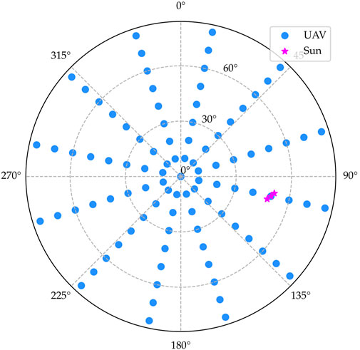
FIGURE 1. Polar plot of observation and illumination geometries.
4.2.3 Atmospheric scattering
Atmospheric scattering is described by two components in this study. First, the molecular atmosphere, modelled using the US Standard atmospheric profile from 1976 (Rodgers, 1976), exhibits Rayleigh scattering. This contributes an aerosol optical thickness (AOT) at 0.55 µm of 0.1. Second, an aerosol layer is added to the atmosphere, which simulates typical aerosol situations in Central Europe. The aerosol distribution was extracted from version 3 of the MAC dataset (Kinne, 2019). The distribution is illustrated in Figure 2. For the AOT at 0.55 µm, the values 0.1 (typical of clear days) and 0.3 [typical high value in Brussels (Sinyuk et al., 2020)] were chosen. Together with a setting that omits atmospheric scattering, this leads to three simulated cases.
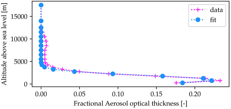
FIGURE 2. Vertical distribution of aerosols, extracted from version 3 of the MAC dataset. The blue line denotes a gaussian fit, with a mean value of 950 m and a standard deviation of 1,030 m.
4.2.4 Calibrated radiometric reference panel
Two cases are considered. In the first one the CRP is an ideal Lambertian surface with a BHR of 100%. In the second case, the CRP is a Spectralon panel with 99% BHR (Georgiev and Butler, 2008).
Unfortunately, Georgiev and Butler (2008) provide data only in the principal plane. To overcome this limitation, a fit of the MVBP model (Pinty et al., 1990) to the provided data is performed. The resulting parameters of the model are given in Table 1 and a comparison of the fit to the principal plane data is shown in Figure 3.
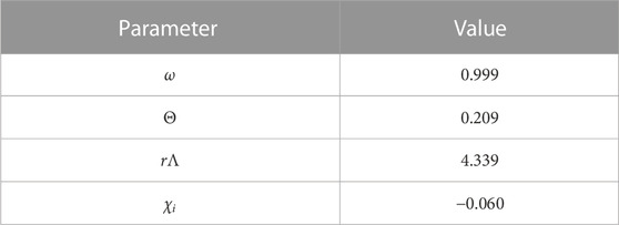
TABLE 1. MVBP parameters obtained by fitting the model to measured Spectralon reflectance at 0.3 µm. Data in Georgiev and Butler (2008) shows minimal variation in the material BRDF between 0.3 µm and 0.55 µm.
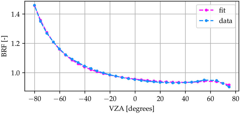
FIGURE 3. The principal plane BRF of the best fit of the MVBP model to the simulated reference panel data for a SZA value of 60°. Negative VZA values correspond to forward scattering. The BRF shows a strong tendency for forward scattering. Note that the BRF at the nadir is not 99%.
At this Sun zenith angle (SZA) value, the BRF of the CRP shows pronounced anisotropy, especially a strong tendency for forward scattering, as well as a slight back-scattering hotspot. Note that the reflectance at the nadir is not 99%. The assumption of 99% reflectance only holds if the total hemispherical reflectance is considered. This is critical, as this study adopts a measurement procedure from related literature (Latini et al., 2021). Here two measurements of the reference panel are taken, from the nadir, at the beginning and end of the 20-min flight duration. The retrieved reflectances are averaged. The actual nadir reflectance for this material is closer to 95%, which means, that unless special care is taken and the actual reflectance value is considered, this measurement approach will overestimate reflectance in the field.
4.3 Illumination
Sun displacement in the sky during the 20-min duration of the UAV flight is simulated by 3 points, shown in Figure 1. To approximate the continuous displacement of the Sun, its position is interpolated linearly between those three fixed points. For all simulations that do not consider the Sun’s movement, the central point (50.0, 0.0) is used for the illumination direction.
4.4 Vegetated surface
The surface in this study is designed in two parts, the soil and a layer of vegetation. The soil is modelled using Lambertian scattering, with a reflectance of 0.1 at 0.55 µm. The vegetation layer is created with a procedural model, which approximates grass (Govaerts, 1995). The individual blades of grass are modelled using bilambertian scattering, with a reflectance of 0.14 and a transmittance of 0.09 at 0.55 µm. The vegetated surface extends 40 m in all directions, which ensures, that the entire visible surface is covered in vegetation for all simulated geometries. Figure 4 shows the grass model rendered from both a very short and a very long distance.
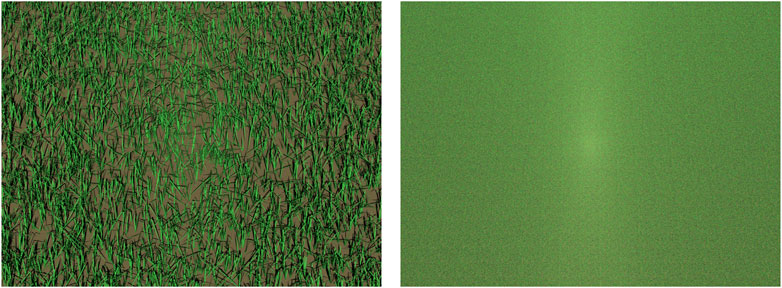
FIGURE 4. The grass surface rendered with a 20° FOV from a (left) 3 m and (right) 120 m distance, without an atmosphere. The solar zenith angle is equal to 50° and the camera points in the back scattering direction. The 120 m-distance view shows the back scattering hotspot, very visible due to the absence of an atmosphere in these simulations. The grass is created procedurally, with parametrizable distributions for the number of segments to each blade and the angle between the segments. Tufts, made up of several blades, are scattered randomly on the surface. Created with eradiate.eu.
4.5 UAV observation
To acquire the surface’s reflectance field, the hemisphere of outgoing directions is sampled every 10° for the zenith angles and 30° for the azimuth angles (Pan et al., 2020; Latini et al., 2021). These sampling densities correspond to 9 points along the viewing zenith angle (VZA) dimension and 12 points along the viewing azimuth angle (VAA) dimension. The sensor is pointed at the same location in the vegetated surface for all simulations and the footprint therefore changes with viewing geometry. Figure 1 illustrates the measurement geometries as well as the positions of the Sun over the 20-min period mentioned above.
4.6 Reference case
The simulated UAV observations, in which the HCRF is retrieved, are compared to a reference case in which access to the true BRF (Eq. 2) of the vegetated surface describe in Section 4.4 is guaranteed. This reference BRF, denoted REF in the following, is the quantity we want to have a proxy for through the HCRF. It is obtained through a simulation under ideal conditions, that is perfectly directional illumination at 50° zenith and 0° azimuth, in the absence of a participating medium and using a perfectly directional sensor.
4.7 Parameter combinations
The combinations of the four parameters chosen for this study (FOV, UAV flight duration, CRP, atmospheric scattering), lead to a total number of 24 simulated scenarios plus the reference BRF simulation. Since the combination of measured CRP and instantaneous acquisition is omitted, the number of scenarios reduces to 18. To help identify the different scenarios, each parameter’s values were assigned letters and each scenario is denoted by a combination of four letters.
Table 2 lists all parameter combinations and their respective shorthand. For further clarification on how the shorthand names are composed, Figure 5 details an example. For example, the scenario in which the parameters are closest to the reference case described in Section 4.6, with Lambertian CRP, static solar position, narrow FOV and no atmosphere would have a shorthand of LINN. The scenario in which the parameters are furthest from the reference case, with a Spectralon measured CRP, moving Sun, a wide FOV and a thick atmosphere would have a shorthand of MRWH. All possible combinations of the parameters were simulated. The only exception is the combination of the non-Lambertian CRP at instantaneous retrieval. The reason for simulating the non-Lambertian CRP is to assess the influence of the variation in reflectance due to the changing illumination across the time of flight of the UAV.
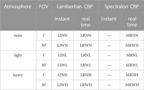
TABLE 2. Shorthand notations for the 18 simulated scenarios and their parameter combinations. The fist letter denotes the type of reference surface, the second letter denotes the acquisition time, the third letter denotes the measurement device’s FOV and the fourth and final letter denotes the type of atmospheric scattering.
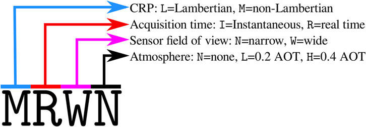
FIGURE 5. Shorthand notations for simulated scenarios. The first position describes the CRP variants, where L denotes the Lambertian CRP and M denotes the non-Lambertian CRP. The second position holds information on the acquisition time. Here, I denotes instantaneous acquisition, while R denotes real-time acquisition. The third position describes the sensor FOV, where N denotes a narrow FOV and W denotes a wide FOV. Finally, the fourth position describes the atmosphere. Here N denotes the absence of atmosphere, L denotes an atmosphere with an AOT of 0.2 and H denotes an atmosphere with an AOT of 0.4.
5 Simulation execution
5.1 The eradiate radiative transfer model
Simulations were performed with the Eradiate radiative transfer model (RTM), an open-source 3D Monte Carlo ray-tracing model, which supports explicit 3D geometry and vegetation as well as complex multi-component atmospheric models (Leroy et al., 2022). Its comprehensive Python interface makes it ideally suited to simulate a set of varying scenes with changing parameters such as the campaign described here.
5.2 Reference case simulation
To simulate the reference case, defined in Section 4.6, the reflected radiance is computed with zenith and azimuth angle steps of 1°. The irradiance from the Sun is known for the simulation and can therefore be used to compute the BRF as defined in Eqs 1, 2, as no atmospheric scattering and absorption are accounted for. Eradiate automates this process and outputs the BRF directly.
5.3 UAV observations
As mentioned in Section 3.2.3, reflectance values are computed as the ratio between the observed radiance reflected by the scene and the CRP. The reflectance is defined as
where Lveg is the reflected radiance from the vegetated surface and LCRP is the reflected radiance from the CRP. This approach can be motivated from Eq. 1 directly. For individual incident and exitant directions the derivative becomes the ratio. Under the assumption, that the CRP reflects light in a perfectly Lambertian manner, the reflected radiance from the panel can be identified as the incident irradiance in the BRDF definition.
The CRP is represented by a square shape of 1 m squared, with the scattering properties of either the fitted MVBP model (Section 4.2.4) or a Lambertian model.
The UAV observations are simulated using a sensor that emulates a multi-pixel perspective camera, positioned in the scene and pointing towards the ground. Since the FOV is fixed, the surface area which is visible in the rendered image changes with the sensor’s position. The multi-pixel images are averaged to produce one radiance value for the chosen observation geometry. This emulates a radiometer with a finite FOV, which records only one value. Two advantages of this approach are that the pixels lead to a stratification of the samples across the sensor plane and that the recorded radiance can be filtered by pixels. The former reduces variance, while the latter allows for cropping of the image to exclude regions of unwanted radiance, such as radiance entering the sensor directly from the sky, which can occur at large values of VZA.
The fixed FOV of the sensor introduces a problem. In oblique observation geometries, radiance from unwanted directions, such as the sky, can enter the sensor. A possible solution to this issue is manual cropping of the images, to exclude contributions from undesired directions. However, in a simulated campaign, cropping can be automated, by creating a mask, which is applied to the images.
The mask for the canopy simulations is created by replacing the vegetated surface with a flat surface with 100% Lambertian reflectance and removing the atmosphere. This will yield an image, which records high radiance values everywhere, where there is vegegation in the original image and zero radiance for the sky. Figure 6 illustrates an oblique observation for the canopy and the corresponding simulated mask.
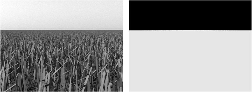
FIGURE 6. Left: A simulated canopy image, recorded at an oblique angle. A significant part of the image records radiance originating from scattering in the atmosphere. Right: A render of a white surface without an atmosphere. Note how the position of the horizon on the left coincides with separating line between the white and black areas on the right. The right image is used to mask the left and crop out unwanted radiance. Created with eradiate.eu
For the simulations of the CRP, the required cropping region is smaller. In this case, the mask is simulated by setting the reflectance of the soil and the canopy to zero and removing the atmosphere. The simulated image will show non-zero radiance values only for the pixels, which contain the CRP.
The deviation Dr of each scenario from the REF case is defined as the relative difference
where RBRF and RHCRF are defined by Eqs 2, 6. The overall deviation of the different scenarios from the REF case was quantified by using the relative root mean squared error between each scenario’s results and the reference BRF:
6 Results
6.1 Reference case
The result of the simulations performed for the REF case are presented in Figure 7, which shows the RBRF reference reflectance values defined in Eq. 7. This quantity is the surface FRM defined in Eq. 2.
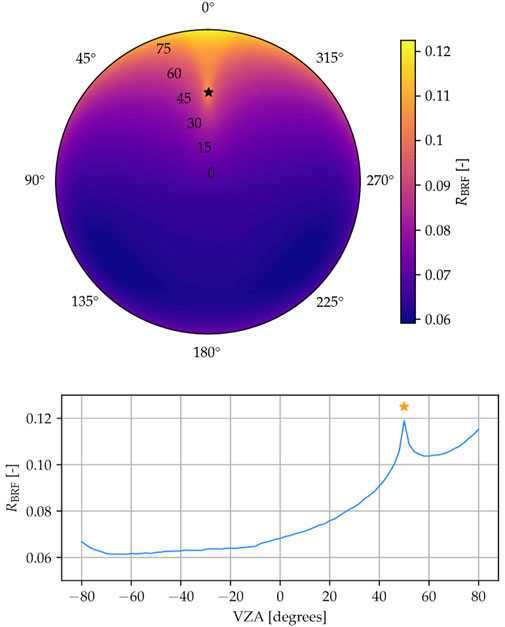
FIGURE 7. Simulated BRF for the REF case. Top: The full hemisphere. Bottom: The principal plane (negative azimuth values correspond to 180° viewing azimuth angle). Stars indicate the direction of illumination. The back scattering hotspot typical of vegetated surfaces is clearly visible.
The overall shape of the reflectance profile is dominated by the back-scattering hotspot (here at 50° zenith angle) typical of vegetated surfaces. The BRF shows high symmetry with respect to the principal plane, which is attributable to the statistical isotropy and uniformity of the vegetated cover.
The lower frame in Figure 7 shows the principal-plane transect of the overall reference BRF. As this typically contains the most distinct features of the BRF, the results of the simulated scenarios provided in the following sections will be similarly provided. However, all statistical quantities and relative differences between the scenarios and the reference are computed across all geometries listed in Section 4.5.
6.2 Narrow FOV (**N* scenarios)
The Lambertian CRP with a narrow FOV and instantaneous acquisition cases (LINN, LINL, LINH in Table 2) are presented first (Figure 8). The LINL and LINH cases illustrate the effects of atmospheric scattering on the HCRF values: increasing levels of atmospheric scattering result in a less intense hotspot in the profile.
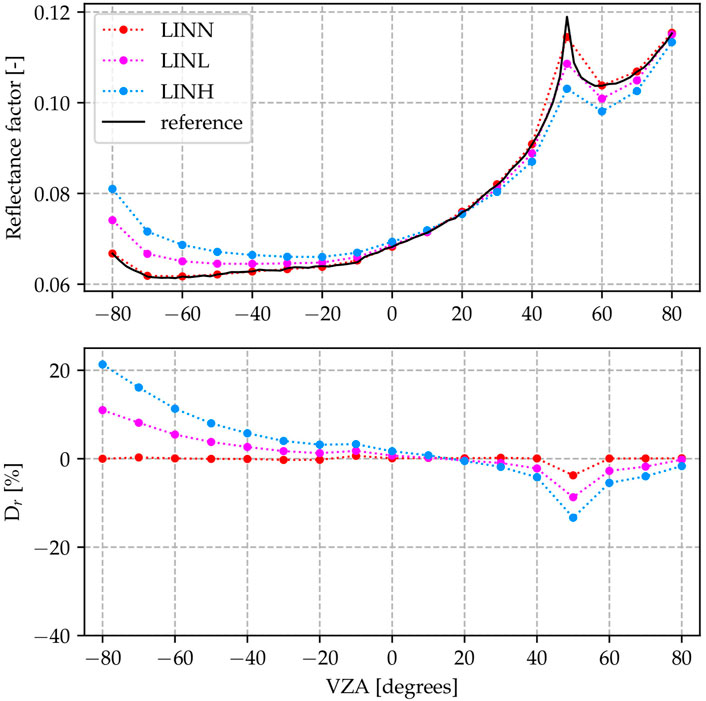
FIGURE 8. Results for the LIN* scenarios (Lambertian CRP, instantaneous acquisition and narrow FOV, varying atmospheric density). The LINN scenario matches the reference well, but the deviation increases with increasing atmospheric density.
The results for the scenarios with Lambertian CRP but non-zero acquisition time (LRN*) are shown in Figure 9. Visually these results differ only by a very small amount from those of the instantaneous acquisition scenarios (LIN*, Figure 8). Figure 10 shows the results for the MRN* scenarios, which include the non-Lambertian CRP. Compared to the LRN* and LIN* scenarios, the observed reflectance values are overall higher.
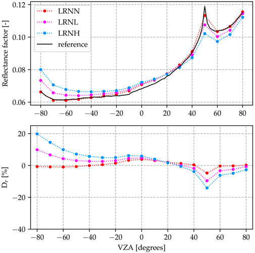
FIGURE 9. Results for the LRN* scenarios (Lambertian CRP, real acquisition time and narrow FOV, varying atmospheric density). The scenario data is lowered near the back-scattering hotspot, compared to the reference result. The difference to the reference increases with increasing atmospheric density.
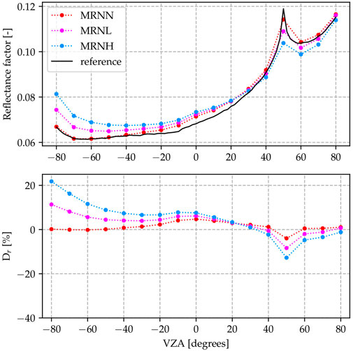
FIGURE 10. Results for the MRN* scenarios (non-Lambertian CRP, real acquisition time and narrow FOV, varying atmospheric density). Note the slight overall increase in values, as compared to the LRN* scenarios.
6.3 Wide FOV (**W* scenarios)
The different atmospheric variants for the wide FOV and otherwise ideal conditions, are shown in Figure 11. The high relative difference values in the back scattering direction suggest that simulations performed with such a wide FOV result in a poorly resolved hotspot. Quantitatively this results in an increased maximum Dr, which is higher than 13% for all cases, whereas it is below 5% for narrow field of view in the **N* scenarios.

FIGURE 11. Results for the LIW* scenarios (Lambertian CRP, instantaneous acquisition and wide FOV, varying atmospheric density). The back-scattering hotspot is much less resolved, than in the reference result.
Combining the wide FOV with the realistic flight duration yields the LRW* scenarios, which are shown in Figure 12. The changes in ΔRRMSE and maximum Dr, compared to the instantaneous scenarios (LIW*) is small. While ΔRRMSE decreases slightly, the maximum Dr increases.
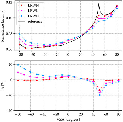
FIGURE 12. Results for the LRW* scenarios (Lambertian CRP, real acquisition time and wide FOV, varying atmospheric density). The back-scattering hotspot is much less resolved, than in the reference result. The difference to the reference result increases with atmospheric density.
Finally, the wide FOV scenarios with the non-Lambertian reference panel (MRW*) are shown in Figure 13. Between the LRW* scenarios and these, ΔRRMSE and maximum Dr,i increase for the no atmosphere scenario, but decrease significantly for the atmosphere scenarios.
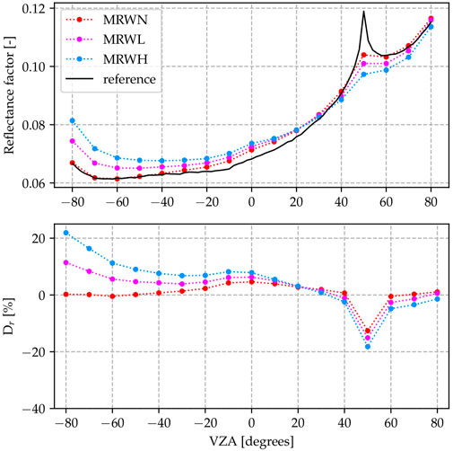
FIGURE 13. Results for the MRW* scenarios (non-Lambertian CRP, real acquisition time and wide FOV, varying atmospheric density). Note the slightly increased reflectance, compared to the LRW* scenarios. The back-scattering hotspot is much less resolved, than in the reference result. The difference to the reference case increases with atmospheric density.
Figures of the reflectances for all scenarios are available as Supplementary Material.
7 Discussion
As expected, the ΔRRMSE is smallest for the LITN scenario (0.4%), because the conditions encountered in this scenario (Lambertian CRP, instantaneous acquisition, tight sensor FOV, no atmosphere) are most similar to the conditions under which the BRF of the REF case is simulated. The largest, appears for the MRWH (non-Lambertian CRP, non-zero time of flight, wide sensor FOV, heavy atmosphere) scenario (8.7%). The influence of various parameters is quantitifed by evaluating the change in mean RRMSE and maximum deviation when changing a single parameter (Table 3). For example, adding light atmosphere means, in terms of scenario abbreviations, ***N → ***L.
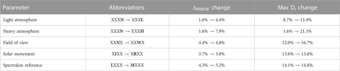
TABLE 3. Average increase in ΔRRMSE and maximum deviation for all parameters.
The measurement device’s FOV is found to have a significant impact. Here the values of 1° and 30° FOV were simulated. While the former might be an overly idealized situation for a real measurement device, the latter is typical for reviewed field measurement campaigns (Li et al., 2021b; Pan et al., 2020; Li et al., 2021a). Although the mean increase in ΔRRMSE when increasing the FOV is rather low at 0.4 percentage points, the maximum deviation increases by a significant amount (4.7 percentage points). In the individual cases it is found that a wide FOV under otherwise idealized conditions, the LIWN scenario, leads to a mean ΔRRMSE of 1.3% with a maximum deviation of around 13%. A close look at Figure 11 reveals that a measurement device with such a large FOV performs poorly at recording the back-scattering hotspot of the surface, even when an idealized case with no atmosphere is considered. Figure 4 can assist in the interpretation of these results: On this image, which shows a wide FOV (20°) render of the surface, the back scattering hotspot is visible. A wide FOV observation is equivalent to averaging all pixels in this image, which results in pixels near the hotspot being blended with the pixels outside the hotspot; in other words, the overall measured value contains the hotspot signal, but is muted due to contributions from adjacent pixels. On the other hand, an observation with a narrow FOV is equivalent to considering only the central portion of the image, which, in practice, means restricting the contributions to the measurement to the near-hotspot pixels.
The largest contribution to bias between HCRF and BRF originates from the scattering of light in the atmosphere. The atmosphere parametrization used for these simulations includes a molecular component featuring Rayleigh scattering (0.1 optical thickness (OT) in the considered spectral band), to which is added an aerosol component with an OT of 0.1 (***L scenarios) or 0.3 (***H scenarios), thus amounting for a total optical of 0.2 (***L scenarios) or 0.4 (***H scenarios). Already with a total OT of 0.2, typical of clear days, the mean ΔRRMSE increases by 3.5 percentage points. With a total OT of 0.4, typical of more hazy days, the mean ΔRRMSE increases by 7 percentage points. In the LINH scenario (ideal CRP, instantaneous acquisition, narrow FOV, atmosphere with 0.4 OT), the HCRF significantly deviates from the reference BRF with a RRMSE of 7.6% and a maximum deviation of 21.3% recorded in the back scattering direction. In the LINL scenario (similar with 0.2 OT, typical of clear days), the RRMSE (4.2%) and maximum deviation (11%), recorded in the back scattering direction are still high.
The celestial movement of the Sun is found to have a minor influence on the difference between HCRF and BRF with a mean increase in ΔRRMSE of 0.1 percentage points. Here, a look at the corresponding scenario LRTN, which uses idealized conditions aside from the solar movement, reveals a mean bias of 1.5% with a maximum deviation of 4.8%.
In terms of ΔRRMSE, the biggest deviation of 8.7% appears at the MRWH scenario, which implements the least ideal conditions. The highest maximum deviation at 21.9% occurs in the MRWH and LIWH scenarios, which further emphasizes the importance of atmospheric scattering.
8 Conclusion and outlook
This study illustrates the challenges of surface BRF estimation from UAV-borne observations. As the BRF is a purely theoretical quantity, in situ measurements can only approximate it and the HCRF should be chosen as the more appropriate quantity. The analysis relies on simulated UAV observations over a grassland with the open-source 3D radiative transfer model Eradiate.
If bottom of atmosphere measurements are to be used as FRMs, being able to estimate the uncertainty of the retrieved surface reflectance is essential. The variables and parameters of such a measurement approach have been discussed and a subset of four parameters with high expected impact on the HCRF acquisition has been selected. For those four parameters, the atmosphere, the FOV of the measurement device, the celestial movement of the Sun and the non-Lambertian reflectance of reference surfaces, typical and realistic values were chosen based on a literature review.
In the presented experimental plan, the acquisition of the HCRF of a highly realistic scene is recreated under different conditions. The bias for each scenario, determined through comparison with a reference BRF of the scene, is computed and from all scenarios the mean effect of each parameter is extracted (See Table 3). In each row the effect of one parameter is given, with the parameter name in the first column and the corresponding shorthands in the second. Here the two letters in bold print denote the parameters which were fixed, while capital X denotes a placeholder, as all variants were averaged. For example XXXN means LINN, LIWN, LRNN, LRWN, MRNN, and MRWN.
Based on the results of this simulation campaign, we issue recommendations for the preparation of future efforts aiming at retrieving BRF records through in situ HCRF retrievals: (i) perform the measurements at a date and time when atmospheric conditions are most favorable, i.e., diffuse sky radiation is as low as possible, and (ii) crop images acquired by UAVs and used for HCRF estimation to keep the effective FOV as small as possible. Recommendation (i) ensures that the illumination is as close as possible to an ideal directional light source, while recommendation (ii) ensures that the sensor is as close as possible to a directional radiance meter. Although meeting the ideal conditions of the reference BRF simulation case (perfectly directional illumination and sensor) is impossible, based upon our results this approach will minimize the magnitude of the issues encountered when attempting to use field HCRF estimations as a proxy for surface BRFs.
Future developments could include the design of a protocol to retrieve the intrinsic surface BRF from bottom of atmosphere HCRF measurements, based on available data characterizing the atmosphere at the date and time of the acquisition. This should be facilitated if the aforementioned recommendations are applied.
Data availability statement
The raw data supporting the conclusion of this article will be made available by the authors, without undue reservation.
Author contributions
SS: Software, Visualization, Writing–original draft, Data curation, Investigation, Methodology. VL: Supervision, Writing–review and editing. YG: Conceptualization, Funding acquisition, Investigation, Methodology, Project administration, Writing–review and editing, Supervision.
Funding
The author(s) declare financial support was received for the research, authorship, and/or publication of this article. This project has received funding from the European Union’s Horizon 2020 research and innovation programme under the grant agreement No. 101004242 (Copernicus CAL/VAL Solution).
Conflict of interest
Authors SS, VL, and YG were employed by Rayference SRL.
Publisher’s note
All claims expressed in this article are solely those of the authors and do not necessarily represent those of their affiliated organizations, or those of the publisher, the editors and the reviewers. Any product that may be evaluated in this article, or claim that may be made by its manufacturer, is not guaranteed or endorsed by the publisher.
Supplementary material
The Supplementary Material for this article can be found online at: https://www.frontiersin.org/articles/10.3389/frsen.2023.1285800/full#supplementary-material
References
Abdou, W. A., Helmlinger, M. C., Conel, J. E., Bruegge, C. J., Pilorz, S. H., Martonchik, J. V., et al. (2001). Ground measurements of surface BRF and HDRF using PARABOLA III. J. Geophys. Res. Atmos. 106, 11967–11976. doi:10.1029/2000JD900654
Bouvet, M., Thome, K., Berthelot, B., Bialek, A., Czapla-Myers, J., Fox, N., et al. (2019). Radcalnet: a radiometric calibration network for earth observing imagers operating in the visible to shortwave infrared spectral range. Remote Sens. 11, 2401. doi:10.3390/rs11202401
Bruegge, C. J., Stiegman, A. E., Rainen, R. A., and Springsteen, A. W. (1993). Use of Spectralon as a diffuse reflectance standard for in-flight calibration of earth-orbiting sensors. Opt. Eng. 32, 805–814. doi:10.1117/12.132373
Burkart, A., Aasen, H., Alonso, L., Menz, G., Bareth, G., and Rascher, U. (2015). Angular dependency of hyperspectral measurements over wheat characterized by a novel uav based goniometer. Remote Sens. 7, 725–746. doi:10.3390/rs70100725
Coll, C., Niclòs, R., Puchades, J., García-Santos, V., Galve, J. M., Pérez-Planells, L., et al. (2019). Laboratory calibration and field measurement of land surface temperature and emissivity using thermal infrared multiband radiometers. Int. J. Appl. Earth Observation Geoinformation 78, 227–239. doi:10.1016/j.jag.2019.02.002
Deng, L., Chen, Y., Zhao, Y., Zhu, L., Gong, H.-L., Guo, L.-J., et al. (2021). An approach for reflectance anisotropy retrieval from UAV-based oblique photogrammetry hyperspectral imagery. Int. J. Appl. Earth Observation Geoinformation 102, 102442. doi:10.1016/j.jag.2021.102442
Georgiev, G. T., and Butler, J. J. (2008)., 7081. SPIE, 46–54. doi:10.1117/12.795931Brdf study of gray-scale spectralonEarth Obs. Syst. XIII
Govaerts, Y. M. (1995). A Model of light Scattering in three-dimensional plant canopies: a Monte Carlo ray tracing approach. Ph.D. Thesis, université catholique de Louvain. Ph.D. Thesis.
Goyens, C., De Vis, P., and Hunt, S. E. (2021). “Automated generation of hyperspectral fiducial reference measurements of water and land surface reflectance for the hypernets networks,” in 2021 IEEE international geoscience and Remote sensing symposium IGARSS (Germany: IEEE), 7920.
Grenzdörffer, G. J., and Niemeyer, F. (2012). Uav based brdf-measurements of agricultural surfaces with pfiffikus. In Int. Archives Photogrammetry, Remote Sens. Spatial Inf. Sci. (Copernicus GmbH),vol. XXXVIII-1-C22, 229–234. doi:10.5194/isprsarchives-xxxviii-1-c22-229-2011
Hutton, J. J., Lipa, G., Baustian, D., Sulik, J., and Bruce, R. W. (2020). High accuracy direct georeferencing of the altum multi-spectral uav camera and its application to high throughput plant phenotyping. Int. Archives Photogrammetry, Remote Sens. Spatial Inf. Sci. XLIII-B1-2020, 451–456. doi:10.5194/isprs-archives-XLIII-B1-2020-451-2020
Jacquemoud, S., and Baret, F. (1990). Prospect: a model of leaf optical properties spectra. Remote Sens. Environ. 34, 75–91. doi:10.1016/0034-4257(90)90100-z
Jurado, J. M., Jiménez-Pérez, J. R., Pádua, L., Feito, F. R., and Sousa, J. J. (2022). An efficient method for acquisition of spectral BRDFs in real-world scenarios. Comput. Graph. 102, 154–163. doi:10.1016/j.cag.2021.08.021
Kinne, S. (2019). The macv2 aerosol climatology. Tellus B Chem. Phys. Meteorology 71, 1623639–1623721. doi:10.1080/16000889.2019.1623639
Latini, D., Petracca, I., Schiavon, G., Niro, F., Casadio, S., and Del Frate, F. (2021). UAV-based observations for surface BRDF characterization. 8193–8196. doi:10.1109/IGARSS47720.2021.9554496
Leroy, V., Nollet, Y., Schunke, S., Misk, N., and Govaerts, Y. (2022). Eradiate radiative transfer model. doi:10.5281/zenodo.7224315
Li, L., Mu, X., Qi, J., Pisek, J., Roosjen, P., Yan, G., et al. (2021a). Characterizing reflectance anisotropy of background soil in open-canopy plantations using UAV-based multiangular images. ISPRS J. Photogrammetry Remote Sens. 177, 263–278. doi:10.1016/j.isprsjprs.2021.05.007
Li, W., Jiang, J., Weiss, M., Madec, S., Tison, F., Philippe, B., et al. (2021b). Impact of the reproductive organs on crop BRDF as observed from a UAV. Remote Sens. Environ. 259, 112433. doi:10.1016/j.rse.2021.112433
Maguire, M. S., Neale, C. M. U., and Woldt, W. E. (2021). Improving accuracy of unmanned aerial system thermal infrared remote sensing for use in energy balance models in agriculture applications. Remote Sens. 13, 1635. doi:10.3390/rs13091635
Milton, E. J., Schaepman, M. E., Anderson, K., Kneubühler, M., and Fox, N. (2009). Progress in field spectroscopy. Remote Sens. Environ. 113, S92–S109. doi:10.1016/j.rse.2007.08.001
Miura, T., and Huete, A. R. (2009). Performance of three reflectance calibration methods for airborne hyperspectral spectrometer data. Sensors (Basel, Switz. 9, 794–813. doi:10.3390/s90200794
Nicodemus, F. E., Richmond, J. C., Hsia, J. J., Ginsberg, I. W., and Limperis, T. (1977). Geometrical considerations and nomenclature for reflectance, 160. Gaithersburg, MD: NBS MONO. doi:10.6028/NBS.MONO.160
Origo, N., Gorroño, J., Ryder, J., Nightingale, J., and Bialek, A. (2020). Fiducial reference measurements for validation of sentinel-2 and proba-V surface reflectance products. Remote Sens. Environ. 241, 111690. doi:10.1016/j.rse.2020
Painter, T. H., Paden, B., and Dozier, J. (2003). Automated spectro-goniometer: a spherical robot for the field measurement of the directional reflectance of snow. Rev. Sci. Instrum. 74, 5179–5188. doi:10.1063/1.1626011
Pan, Z., Zhang, H., Min, X., and Xu, Z. (2020). Vicarious calibration correction of large FOV sensor using BRDF model based on UAV angular spectrum measurements. J. Appl. Remote Sens. 14, 027501. doi:10.1117/1.JRS.14.027501
Pinty, B., Verstraete, M. M., and Dickinson, R. E. (1990). A physical model of the bidirectional reflectance of vegetation canopies: 2. Inversion and validation. J. Geoph. Res. 95, 11767–11775. doi:10.1029/jd095id08p11767
Rodgers, C. D. (1976). Retrieval of atmospheric temperature and composition from remote measurements of thermal radiation. Rev. Geophys. Space Phys 14, 609–624. doi:10.1029/rg014i004p00609
Sandmeier, S., Sandmeier, W., Itten, K., Schaepman, M., and Kellenberger, T. (1995). The Swiss field-goniometer system (FIGOS). In 1995 International Geoscience and remote sensing Symposium, IGARSS ’95. Quantitative remote Sensing for Science and applications. vol. 3, 2078–2080. doi:10.1109/IGARSS.1995.524113
Schaepman-Strub, G., Schaepman, M., Painter, T., Dangel, S., and Martonchik, J. (2006). Reflectance quantities in optical remote sensing—definitions and case studies. Remote Sens. Environ. 103, 27–42. doi:10.1016/j.rse.2006.03.002
Sinyuk, A., Holben, B. N., Eck, T. F., Giles, D. M., Slutsker, I., Korkin, S., et al. (2020). The AERONET Version 3 aerosol retrieval algorithm, associated uncertainties and comparisons to Version 2. Atmos. Meas. Tech. 13, 3375–3411. doi:10.5194/amt-13-3375-2020
Sterckx, S., Brown, I., Kääb, A., Krol, M., Morrow, R., Veefkind, P., et al. (2020). Towards a european cal/val service for earth observation. Int. J. Remote Sens. 41, 4496–4511. doi:10.1080/01431161.2020.1718240
Viallefont-Robinet, F., Bacour, C., Bouvet, M., Kheireddine, M., Ouhssain, M., Idoughi, R., et al. (2019). Contribution to sandy site characterization: spectro-directional signature, grain size distribution and mineralogy extracted from sand samples. Remote Sens. 11, 2446. doi:10.3390/rs11202446
Keywords: fiducial reference measurement, UAV, BRDF, quality control, Earth observation
Citation: Schunke S, Leroy V and Govaerts Y (2023) Retrieving BRDFs from UAV-based radiometers for fiducial reference measurements: caveats and recommendations. Front. Remote Sens. 4:1285800. doi: 10.3389/frsen.2023.1285800
Received: 30 August 2023; Accepted: 30 October 2023;
Published: 20 November 2023.
Edited by:
Agnieszka Bialek, National Physical Laboratory, United KingdomReviewed by:
Dmitry Efremenko, German Aerospace Center (DLR), GermanyRaymond Soffer, National Research Council Canada (NRC), Canada
Andreas Hueni, University of Zurich, Switzerland
Copyright © 2023 Schunke, Leroy and Govaerts. This is an open-access article distributed under the terms of the Creative Commons Attribution License (CC BY). The use, distribution or reproduction in other forums is permitted, provided the original author(s) and the copyright owner(s) are credited and that the original publication in this journal is cited, in accordance with accepted academic practice. No use, distribution or reproduction is permitted which does not comply with these terms.
*Correspondence: Sebastian Schunke, sebastian.schunke@rayference.eu
†ORCID: Sebastian Schunke, orcid.org/0000-0002-5304-2410; Vincent Leroy, orcid.org/0000-0002-5407-0237; Yves Govaerts, orcid.org/0000-0002-9476-9595