Knowledge-informed data-driven modeling for sparse identification of governing equations for microbial inactivation processes in food

1 Introduction

Food is vulnerable to contamination by pathogens and spoilers. Pathogens in contaminated food induce foodborne diseases, while spoilers deteriorate the quality of food by changing the biochemical properties of food materials (Lianou et al., 2016). The invasion of those harmful microorganisms can take place anytime throughout the lifecycle of food including production, processing, distribution, storing, and preservation (Lianou et al., 2016). Treatment of food with extreme conditions is known to render microbes inert, which is however not an ideal solution due to adverse effects on texture, taste, and flavor, denaturation of nutrients (e.g., vitamin A), as well as excessive energy demand (Amit et al., 2017). As complete removal of pathogens and spoilers from food is often infeasible as such, their suppression to a safe low level by refining treatment methods and conditions is essential for ensuring food safety and quality. Therefore, determination of optimal conditions to control the growth of harmful microorganisms requires meeting multiple objectives that are often contradictory (Madoumier et al., 2019). While many alternative microbial inactivation technologies with temperate processing conditions have emerged, such as high-pressure processing (Podolak et al., 2020), pulsed light inactivation (Artíguez et al., 2011), and various non-thermal methods (Mañas and Pagán, 2005), accurate evaluation of the relative influences of the associated process factors remains challenging due to the lack of a tractable and generalizable approach to analyze the process mechanics.

Mathematical models are indispensable tools for predicting and optimizing microbial inactivation processes in food. Accurate modeling of microbial growth or inactivation is a difficult task due its complex dependence on numerous internal (such as water activity, pH, composition, and preservatives) and external food conditions (e.g., temperature and humidity) (Akkermans et al., 2020). Appropriate consideration of the functional relationships between microbial populations and such intrinsic and extrinsic parameters is critical for model performance. Microbial inactivation models are often built on fitted polynomial equations, while other forms such as Arrhenius or square root relationships have also been considered (Whiting, 1995; Ross and Dalgaard, 2003). Typical modeling efforts using the polynomial equations have focused on determining optimal parameter values (i.e., coefficients of pre-chosen terms) through data fit. However, this approach cannot ensure robust development of microbial inactivation models because inadequate representation of equations can lead to poor performance in data fit and prediction due to intrinsic structural error that cannot be compensated through parameter estimation (Kaplan, 2002). Moreover, empirical determination of governing terms often lacks expandability with increasing number of process variables, necessitating a more systematic, rational approach.

Sparse Identification of Nonlinear Dynamics (SINDy) (Brunton et al., 2016) is a promising approach that enables automatic discovery of model equations without having to assume model structure a priori, making it distinct from typical approaches that focus on estimating optimal values of the parameters through data fit in a pre-defined function. SINDy allows the use of a library of input variables (that potentially affect the output variables of interest) to identify the model structure by linear combinations of the terms in the library. Following the Occam’s razor principle postulating that the simplest explanation generally tends to be the correct representation (Blumer et al., 1987; Song et al., 2013), SINDy promotes parsimony in model identification based on a minimal subset of terms.

In this work, we present a data-driven modeling pipeline utilizing SINDy for robust development of microbial inactivation models for application in food safety and quality. While the original goal of SINDy is to identify sparse models of nonlinear dynamical systems, we apply it to non-dynamical systems through appropriate reformulation (see Methods). For demonstration, we considered case studies of modeling the change in D-values—the time taken for a 90% reduction in microbial population—under the variations of multiple factors including temperature, pH, water activity, NaCl content, and phosphate level. Built on SINDy, our modeling pipeline has three major additional features: 1) Incorporation of theoretical knowledge on the relationships between basic input and output variables, e.g., by accounting for the temperature dependence of D-value following the Arrhenius equation; 2) rational determination of hyperparameters (such as the polynomial order and sparsity-controlling parameter) based on information-theoretic metric for an optimal balance between model accuracy and sparsity, and 3) integration with global sensitivity analysis to evaluate the effects of key factors on model outputs. Our analysis showed that the benchmark models in the literature considered in this work are mostly over- or underfitted. Using our approach, therefore, we were able to propose better structured models with improved accuracy and less complexity.

2 Materials and methods

Identification of model structure (i.e., functional forms of the relationship between input and output variables) is challenging as there are many possible solutions to formulate a specific model from a given dataset. In this section, we describe how systematic identification of model equations and key variables/terms governing microbial inactivation can be enabled by an advanced data-driven approach called SINDy (Brunton et al., 2016) in conjunction with global sensitivity analysis, respectively.

2.1 Essence of sparse identification of nonlinear dynamics

The original motivation of SINDy is to discover governing equations for nonlinear dynamical systems, which is reconfigured here to apply to non-dynamical systems as follows:

where $\mathbf{x}$ is the vector of state variables, and $\mathbf{f}$ denotes the nonlinear relationship between the input ($\mathbf{x}$) and output variables ($\mathit{y}$). SINDy approximates $\mathbf{f}$ by a weighted linear combination of nonlinear terms, e.g., for the $i^{th}$ output variable:

where ${\theta }_k\left(\mathbf{x}\right)$ and ${\xi }_{k,i}$ denote the $k^{th}$ term and its weight, respectively. The above equations can be represented in a more succinct form as matrices, i.e.,

where $\mathbf{X}=\left[{\mathbf{x}}_{\mathbf{1}}{\mathbf{x}}_{\mathbf{2}}\cdots {\mathbf{x}}_{\mathbf{m}}\right]$, $\mathbf{Y}=\left[{\mathbf{y}}_{\mathbf{1}}{\mathbf{y}}_{\mathbf{2}}\cdots {\mathbf{y}}_{\mathbf{n}}\right]$, $\mathbf{\Theta }\left(\mathbf{X}\right)$ is a library of candidate functions of $\mathbf{X}$ and the matrix of weights $\mathbf{\Xi }=\left[{\mathit{\xi }}_{\mathit{1}}{\mathit{\xi }}_{\mathit{2}}\cdots {\mathit{\xi }}_m\right]$. In SINDy, the library $\mathbf{\Theta }\left(\mathbf{X}\right)$ is built by polynomial expansion of input variables $\mathbf{X}$, i.e., $\mathbf{\Theta }\left(\mathbf{X}\right)=\left[\mathbf{1}\mathbf{X}{\mathbf{X}}^{\mathit{2}}\cdots {\mathbf{X}}^d\cdots \right]$ where ${\mathbf{X}}^d$ denotes a matrix with column vectors of all possible $d^{th}$degree monomials in the state variable $\mathbf{x}$.

SINDy seeks a parsimonious model composed with minimal number of terms as possible without compromising model accuracy. Sparse regression methods such as Sequentially Thresholded Least Squares (STLS) and Least Absolute Shrinkage and Selection Operator (LASSO) are useful algorithms that can be used in SINDy for this purpose (Brunton et al., 2016). In this work, we employ STLS where $\mathbf{\Xi }$ in Eq. 3 retains the coefficients (weights) greater than the prescribed parameter $\lambda$ (otherwise, zero weights are assigned), such that only the terms in the library with significant influence on the outputs are included in the final model structure. Here, $\lambda$ is known as sparsity-promoting knob because the model sparsity increases with higher values of $\lambda$, while model accuracy may decrease.

2.2 Application of SINDy to microbial inactivation modeling

We use SINDy to formulate microbial inactivation as functions of various process variables including temperature ($T$), pH, water activity ($a_w$), NaCl content ($C_N$), and phosphate level ($C_P$), which are all known to significantly influence microbial growth rate (Juneja et al., 1995; Cerf et al., 1996). We employ D-value (i.e., the time for microbial population to shrink to 10% of initial level) as a standard measure for microbial inactivation, which is taken as our target variable to predict in applying SINDy. With a single target variable chosen, Eq. 3 is reduced to the following equation, i.e.,

While SINDy offers flexibility to pick any nonlinear terms for input and output variables, we determine the inclusion of their specific functional forms following the known mechanistic knowledge and characteristics of the system. Therefore, we used a vector of $\log \mathbf{D}$ as $\mathbf{y}$ (instead of a vector of $\mathbf{D}$) and determined $\mathbf{X}$ to be [$\mathit{1}/\mathbf{T}$, pH, ${\mathbf{a}}_{\mathbf{w}}$, ${\mathbf{C}}_{\mathbf{N}}$, ${\mathbf{C}}_{\mathbf{P}}$] (i.e., the use of 1/T, instead of $\mathbf{T}$). The rationale for our choice of functional forms of output and input variables are detailed in Section 3.1.

2.3 Tuning model sparsity and accuracy based on an information-theoretic criterion

We tune the order of combination of primitive process variables and the sparsity index, $\lambda$, in stages. We first determine the maximum order of combination with $\lambda =\mathit{0}$ (which will result in a non-parsimonious model), beyond which there are no significant improvements to model accuracy. Subsequently, by retaining the maximum polynomial order, we employ the maximum $\lambda$ that does not significantly compromise the model accuracy. To facilitate determining optimal polynomial order and $\lambda$ values for a balanced compromise between model accuracy and sparsity, we use an information-theoretic metric, Akaike Information Criterion (AIC) (Akaike, 1998). Specifically, we use the second-order information criterion that includes a correction term to alleviate the bias that may arise if the number of model parameters is large relative to the sample datapoints (Burnham and Anderson, 2002):

where MSE denotes mean squared error, $n$ is the number of sample datapoints, $K$ is the number of model parameters and the third term on the RHS corrects the bias where it tends to zero when $n\gg K$. Generally, a model with the least AIC score is ideal as AIC penalizes the model based on the relative balance between error and complexity ($K$). The formulation above is often denoted as AICc in the literature. The methodical implementation of the general guidelines to develop microbial inactivation models is demonstrated in Section 3.2.

2.4 Density-based global sensitivity analysis

We perform sensitivity analyses on our models as an alternative to arduous assessment of the relative effects of the process variables on microbial inactivation directly from highly distributed experimental data. As the models are linear combinations of nonlinear terms and the datasets used in this work span over a wide parameter space, the possibility of model forming stiff parameter dependency is high. Therefore, we employ a density-based global sensitivity analysis approach called PAWN (Pianosi and Wagener, 2015), instead of local sensitivity approach. Based on this approach, absolute deviation is calculated between an unconditional cumulative density function of model output, $F\left(y\right)$, where all input variables in the model are randomly sampled simultaneously over the whole parameter space, and conditional cumulative density functions, $F\left(y|{\overline{X}}_{i,k}\right)$, which are constructed by randomly sampling all but a single model variable of interest fixed at the $k^{th}$ nominal value, $X_i={\overline{X}}_{i,k}$. The sensitivity index for $i$-th model variable, $S_i$, is characterized as the maximum value across the distribution of absolute deviations collected for a range of $k$ nominal values:

Here, $KS$ is the Kolmogorov—Smirnov statistic, $y$ is the model-estimated D-values and the variable $X_i$ is the $i^{th}$ element of $\mathbf{X}=\left\{T,\mathrm{p}\mathrm{H},a_w,C_N,C_P\right\}$.

2.5 Experimental datasets

The experimental datasets used for microbial inactivation modeling in this work are collated in Table 1. We chose datasets that are predominantly distinct in terms of microorganisms, media, process variables, and parameter space to demonstrate the tractability of our knowledge-informed data-driven pipeline for model development. We also found that the structure of the literature models developed from these datasets was under- or over-determined, rather than optimally determined. Consequently, the datasets and benchmark models we chose serve as an ideal testbed for evaluating the robustness of our approach.

Table 1. Experimental datasets used in this study.

2.6 Computational implementation

Numerical codes were developed using MATLAB^® R2021a by adapting the prototype codes of SINDy provided in Brunton and Kutz (2019) and PAWN global sensitivity analysis given in Pianosi and Wagener (2015) and Pianosi et al. (2015).

3 Results

3.1 Development of a knowledge-informed data-driven modeling pipeline

Our data-driven modeling approach combines SINDy and global sensitivity analysis to identify model equations and key factors that govern microbial inactivation in food. As a main feature, users can define any functional forms of input variables ($T,pH,a_w,C_N,C_P)$, i.e., $g_T\left(T\right),g_{pH}\left(pH\right),$ $g_{a_w}\left(a_w\right)$, $g_{C_N}\left(C_N\right)$, $g_{C_P}(C_P$), and output variables (i.e., $g_D(D$)). As explained below, we set $g_D\left(D\right)=\log D$ (instead of $D$) and determined $g_T\left(T\right)=\mathit{1}/T$ based on the Arrhenius equation, while using first-order terms for the other input variables, i.e., $g_{pH}\left(pH\right)=pH,$ $g_{a_w}\left(a_w\right)=a_w$, $g_{C_N}\left(C_N\right)=C_N$, and $g_{C_P}\left(C_P\right)=C_P$. Subsequently, a library of input terms is generated through polynomial combinations of those basic input variables provided from the user. SINDy, then, identifies a sparse model by choosing a minimum number of input terms (included in the library) that is required to represent the output variable with an acceptable accuracy (cf. Section 2.1). The resulting equations derived by SINDy takes the form of a linear combination of nonlinear terms, and therefore, explicitly show the impacts of environmental variables on D-values. The impact of individual primitive input variables (not the combined terms) can be identified through PAWN global sensitivity analysis. The two complementary tools together identify key model equations and factors that govern D-value for a given pathogen or spoiler. The modeling workflow is illustrated in Figure 1. We term our approach knowledge-based data-driven modeling as we incorporate known insights of system characteristics (such as Arrhenius equation) as a key component to determine basic form of input and output variables as described in detail below.

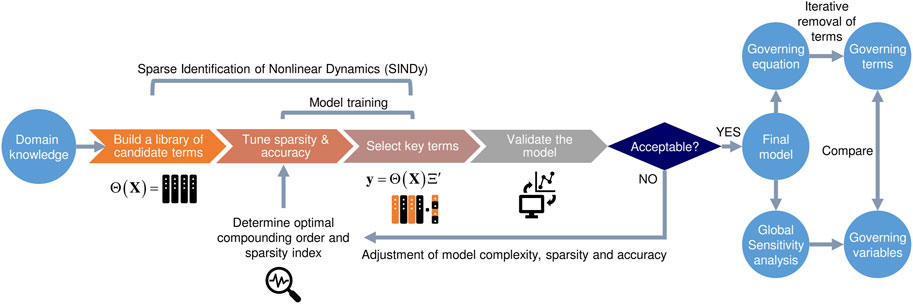
FIGURE 1. Flowchart depicting our knowledge-informed data-driven model development pipeline. The weights assigned to the columns of experimental input variables curated to the functional forms of candidate terms in the library instruct the choice of terms to be included in the final model structure through Sequentially Thresholded Least Squares (STLS) regression (more details in main texts).

The development of data-driven microbial inactivation model can be facilitated by known characteristics of the system. While first-order representation is a typical choice for input and output variables, it is possible to improve model performance by a more appropriate choice of their functional forms. For this purpose, we leverage mechanistic microbial growth models (Whiting, 1995) to inform our choice of functional forms for microbial inactivation dynamics as follows:

where $N$ is population density and $k\left(>\mathit{0}\right)$ is the deactivation rate constant, which is given as a function of a vector of environmental variables ($\mathbf{p}$). If we maintain environmental variables constant over time, we can get the solution in an analytical form, i.e.,

By definition, the population density is $N=\mathit{0.1}{N}_{\mathit{0}}$ when $t=D$, i.e.,

Therefore, D-value is simply:

Subsequently, applying logarithm to the equation above yields:

where $C$ is a constant. Given that many prior Arrhenius-based models produce reasonable fit to growth data by relating the growth rate to various environmental variables as $\ln k=f\left(\mathit{1}/T,pH,a_w,\cdots \right)$ (Whiting, 1995; Ross and Dalgaard, 2003), we similarly re-write Eq. 11 as:

Consequently, the functional forms of output variable and input variables provided for SINDy implementations are $\mathbf{y}=\log \mathbf{D}$ and $\mathbf{X}=\left[\mathit{1}/\mathbf{T},\mathbf{p}\mathbf{H},{\mathbf{a}}_{\mathbf{w}},{\mathbf{C}}_{\mathbf{N}},{\mathbf{C}}_{\mathbf{P}}\right]$ in $\mathbf{\Theta }\left(\mathbf{X}\right)$, respectively, in reference to the generalized form in Eq. 4.

3.2 Optimization of model complexity: Setting polynomial order and model sparsity

To substantiate our choice of functional forms for input and output variables in the preceding section, we compare the model performance per our approach (orange lines in Figure 2) against another base case with non-logarithmic D-values and non-reciprocal temperature and other process variables (blue lines in Figure 2). Here, complete non-parsimonious models are used to ensure fair comparison of the models without the influence of sparse regression. Our approach consistently performed better in terms of MSE calculated based on logarithmic D-values for both cases across different datasets and orders of polynomial combinations of input variables. For all the results that follow henceforth, our choice of the functional forms (i.e., orange lines in Figure 2) are adopted.

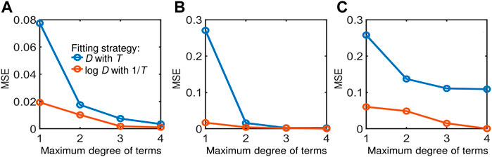
FIGURE 2. Comparison of model performance between different choices of functional forms for input and output variables using datasets from: (A) Cerf et al. (1996), (B) Juneja et al. (1995), and (C) Villa-Rojas et al. (2013). The blue line represents a model with D (chosen as the target variable) and $T,\mathrm{p}\mathrm{H},a_w,C_N,C_P$ (chosen as input variables), whereas the orange line is our choice of functional forms by taking log D as the target variable and $\mathit{1}/T,\mathrm{p}\mathrm{H},a_w,C_N,C_P$ as input variables. The non-parsimonious models ($\lambda =\mathit{0}$) were developed for increasing orders of polynomial combinations of input variables producing monomial terms with various degrees.

With $\log D$ chosen as the target variable, we identify the optimal model structure that balances both accuracy and sparsity. We first determine the order of polynomial combination without accounting for model sparsity (i.e., with $\lambda =\mathit{0}$) and subsequently choose the appropriate value of $\lambda$ (now to promote sparsity). This two-step process is demonstrated through the case study of the dataset from Cerf et al. (1996) (Figures 3, 4). In doing this, we used three major criteria including AIC values, MSE, and the number of terms. The analysis based on the first criterion suggested us to choose the third order polynomial combination (Figure 3A) and $\lambda =\mathit{0}$ (Figure 3B) where the AIC scores are minimal. In contrast, determination of the order of polynomial combination is not clear based on MSE because it keeps decreasing as the order increases (Figure 4A), highlighting the utility of information-theoretic criterion. While the third-order model with $\lambda =\mathit{0}$ may be a desirable choice from a rigorous statistical point of view, we found that the increase of MSE is not significant up to $\lambda =\mathit{1.36}$ (Figure 4B) where the number of terms can be further reduced from 20 to 17 (Figure 4C). MSE was significantly increased when $\lambda >\mathit{1.36}$ without significantly reducing the number of terms, leading us to choose the third-order model with $\lambda =\mathit{1.36}$.

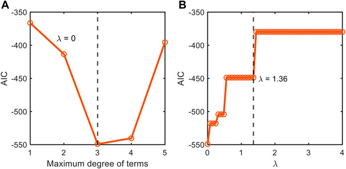
FIGURE 3. Stepwise tuning of model accuracy and sparsity through the comparison of information-theoretic metric (AIC) by first (A) fixing the order of polynomial combinations of input variables for non-parsimonious model ($\lambda =\mathit{0}$), followed by (B) setting the sparsity index, $\lambda$, that balances the model accuracy and desired sparsity. Vertical dashed lines indicate the chosen model settings. Here, the model tuning for dataset from Cerf et al. (1996) is shown as an example.

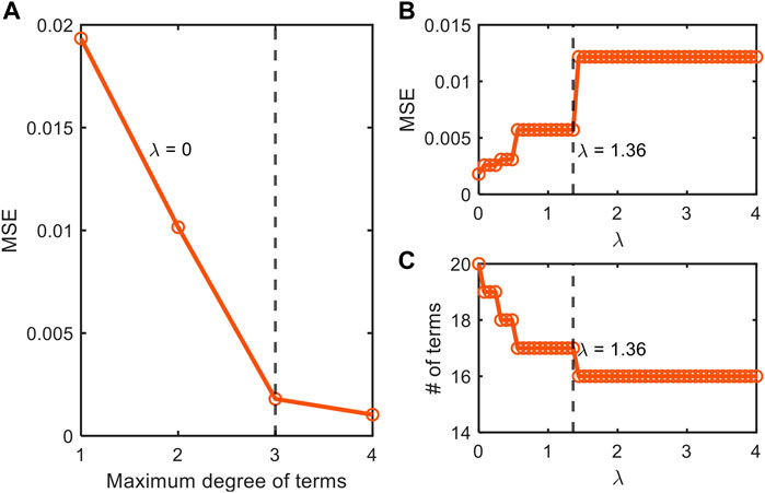
FIGURE 4. Depiction of our stepwise model tuning approach that minimizes model overfitting through the optimization of (A) the order of polynomial combinations of input variables for non-parsimonious model ($\lambda =\mathit{0}$), and (B/C) the sparsity index, $\lambda$. Vertical dashed lines indicate the chosen model settings. Here, the model tuning for dataset from Cerf et al. (1996) is shown as an example.

We also applied this stepwise model construction approach to the datasets from Juneja et al. (1995) (Supplementary Figures S1, S2) and Villa-Rojas et al. (2013) (Supplementary Figures S3, S4). The analysis for the dataset from Juneja et al. (1995) showed that AIC values have two local minima at the polynomial orders 2 and 4 (Supplementary Figure S1A). Through further checking with MSE and the number of terms, we chose the second-order model for better interpretability. After determining the polynomial order, we subsequently determined the optimal value of $\lambda$ to be 0.24 (Supplementary Figure S1B). The changes of MSE and the number of terms as polynomial orders and $\lambda$ values support our choice (Supplementary Figure S2). Lastly, the analysis of the dataset from Villa-Rojas et al. (2013) suggested the first-order model (Supplementary Figures S3, S4), which is because any further increase of model complexity would result in severe overfitting due to limited data points ($n=16$). In this case, we have not further reduced model complexity by fine tuning $\lambda$. The final model was therefore a simple equation with two input variables ($T$ and $a_w$).

3.3 Data-driven identification of governing equations for enhanced accuracy and expandability

Following the guidelines outlined in the preceding and Methods sections, we developed models for all experimental datasets considered in this work. The resulting model equations are summarized in Table 2. The individual models consist of varying number and degree of monomial terms as identified through our data-driven model development pipeline which are optimal to represent the output variable within the parameter space of the respective datasets. The identification of the optimal terms (especially higher-order terms) would not be possible with the previous approaches that rely on empirical choices of equation terms. The issues of model overfitting and uncertainties are also minimized with our stepwise approach in model design.

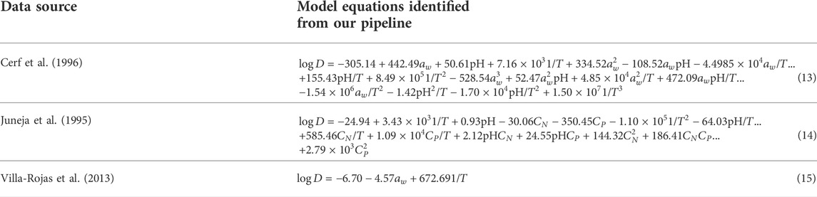
Table 2. Governing model equations identified by leveraging our knowledge-informed data-driven modeling pipeline.

We compare the performance of our models with existing models from the literature in Figure 5. Our models consistently perform better than the literature models across all datasets, particularly for the dataset from Juneja et al. (1995) that has considered additional process variables, i.e., $C_N$ and $C_P$. It is certainly possible that $C_N$ and $C_P$ have significant interaction effects with other process variables and are critical to characterize microbial inactivation dynamics, which explains the enhanced accuracy that accompanies their inclusion in the model. Quantitative information of the models is tabulated in Table 3. In all cases, our models perform adequately with reasonable error measures, i.e., MSE $\le \mathrm{O}\left({\mathit{10}}^{-\mathit{2}}\right)$ and low AIC scores. In two of the cases (models for datasets from Juneja et al. (1995) and Villa-Rojas et al. (2013)), our models gained more than ten-fold increase in accuracy with fewer number of functional terms in the model structures as compared to the literature models. Moreover, we demonstrate the opportunity to further enhance the model accuracy over two-folds for dataset from Cerf et al. (1996) by considering a more complex model equation (greater number of functional terms) without the risk of overfitting as shown by the lower AIC score as compared to the literature model. By carefully adopting the stepwise model tuning scheme as described in Section 3.2, we were able to optimally tune the models to achieve better accuracy while minimizing the chances of overfitting as compared to existing literature models.

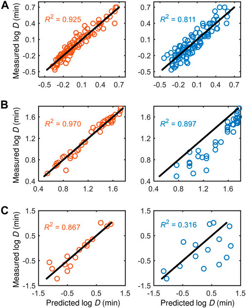
FIGURE 5. Comparison of the performance of our knowledge-informed data-driven models (left panels) against literature models (right panels) across different datasets: (A) Cerf et al. (1996), (B) Juneja et al. (1995), and (C) Villa-Rojas et al. (2013).

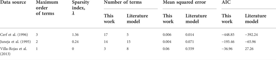
Table 3. Quantitative performance measures of models.

3.4 Integration of data-driven approach and sensitivity analysis for determining key governing process variables and model terms

While our model governing equations offer good representations of experimental data, the individual effects of process variables remain elusive. In addition to data-driven modeling, we leverage global sensitivity analysis (Pianosi and Wagener, 2015) using the model-derived governing equations to identify key governing process variables and possibly divulge the interactions between them. Here, the sensitivities are evaluated for the entire parameter space encompassed by the respective datasets (Table 1). Our results demonstrate highly disparate sensitivity measures for the process variables across datasets as shown in Figure 6, positing that the relative effects of the process variables may be highly environment dependent. For example, $T$ exhibited high sensitivity in the model for data from Cerf et al. (1996) but registered lower sensitivity than other process variables in the model for data from Juneja et al. (1995), although $T$ is often viewed as the primary process variable in most microbial inactivation experiments. Conversely, $a_w$ consistently displayed relatively lower sensitivity measures than other process variables across the models. While condition-specificity is one of the plausible explanations for contrasting sensitivity measures, it should also be noted that the global sensitivity analysis strictly represents the individual influence of process variables on output and are indifferent to interactions effects between process variables. Therefore, there may be instances where the sensitivity measures of the individual process variables are insignificant, whilst considerable interactions effects with other process variables exist. For instance, $T$ and pH registered low sensitivity in the model for data from Juneja et al. (1995) with statistically insignificant influence on the output variable (Figure 6), but the variables were repeatedly included in numerous terms in the governing equation identified through our knowledge-informed data driven approach (Table 2). This is expected given that SINDy retains the most influential terms irrespective of individual or interaction effects necessary for representation of output data.

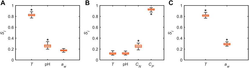
FIGURE 6. Distribution of global sensitivities of process variables on output variable, i.e., $\log D$, examined using models derived from different datasets: (A) Cerf et al. (1996), (B) Juneja et al. (1995), and (C) Villa-Rojas et al. (2013). The symbol * marks the model variables with significant influence on the output based on 95% confidence interval ($\mathrm{p}<0.05$).

To resolve this issue, we implement the combined use of data-driven approach and global sensitivity analysis that enables elucidation of the factors influencing the process dynamics from the contexts of governing equations, key process variables and critical model monomial terms. To this effect, we iteratively removed each term in the governing equations, and subsequently refitted the models with new MSEs as shown in Figure 7, whereby considerable increase in MSE (as compared to the original complete model, represented by horizontal dashed lines) indicates that the respective terms are essential to represent the output variable. In the model for data from Cerf et al. (1996), removal of terms containing $\mathrm{p}\mathrm{H}$ and $a_w$ results in considerable increase in MSEs though the variables had relatively insignificant influences on the output in global sensitivity analysis. Clearly, $\mathrm{p}\mathrm{H}$ and $a_w$ significantly influence the effects of $T$ on microbial inactivation through strong interaction effects, but the reverse is not necessarily true. The finding here is reinforced by the outcome from SINDy, where the terms with $\mathrm{p}\mathrm{H}$ and $a_w$ were unequivocally retained in the governing equations despite diminished main effects (individual effects), as the variables are still relevant to represent the output through their influence on $T$. Therefore, users can, hypothetically, fix the $\mathrm{p}\mathrm{H}$ and $a_w$ at arbitrary optimal levels and tune only $T$ as an alternative reduced-order experimental optimization.

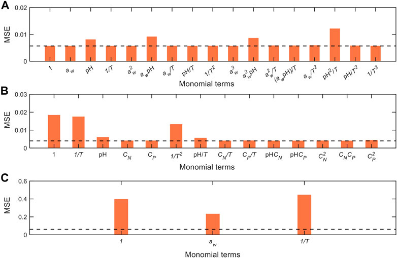
FIGURE 7. Comparison of model performance with iterative removal of terms from the model equations generated from different datasets: (A) Cerf et al. (1996), (B) Juneja et al. (1995), and (C) Villa-Rojas et al. (2013). MSEs are recalculated after refitting the model with the removal of each term, whereby a large increase in MSEs indicates that the respective terms are highly critical to represent the output data. The MSEs of the original complete model are denoted by the horizontal dashed lines (cf. MSEs in Table 3).

Conversely, in the model for data from Juneja et al. (1995), removal of terms with $C_N$ and $C_P$ does not significantly increase the MSE despite their elevated global sensitivity. Therefore, the effects of $C_N$ and $C_P$ on microbial inactivation are possibly dependent on other process variables but they do not impose similar magnitudes of influence in return. Nevertheless, SINDy has retained the terms with $C_N$ and $C_P$ as their substantial individual effects are critical to represent the output when other process variables are invariant. For this system, a stepwise process optimization will work best where $T$ and $\mathrm{p}\mathrm{H}$ is independently tuned first followed by the optimization of $C_N$ and $C_P$. Lastly, the model for data from Villa-Rojas et al. (2013) is fairly simple where both involved process variables possibly impose equivalent individual and interaction effects. While the global sensitivity analysis and reassessment of MSEs with iterative removal of terms offer additional insights that can aid process optimizations, we do not recommend the users to influence the model selection through these insights as they are model-derived contextual outcomes, and thus, the model should be thoroughly optimized beforehand, through the iterative feedback loop (Figure 1) as desired.

4 Discussion

Conventional modeling approaches that empirically ascertain model structures and parameter functional forms are forceful approximations as there exists an overwhelmingly large number of possible solutions. Using a systematic data-driven model development pipeline guided by knowledge-informed choices of parameter functional forms and methodical tuning of model sparsity and accuracy, we developed microbial inactivation models that outperformed existing models from the literature. Our approach not only ensures identifying the most plausible model structure by leveraging on domain knowledge of the system, but also elucidates the factors affecting the process dynamics through the combined use of global sensitivity analysis.

The sound choice of functional forms for input and output target variables as informed by mechanistic formulation (e.g., Arrhenius equation in this work) can be integral in optimizing model structure and performance. The inclusion of the reciprocal functional form for temperature is fitting as it resembles the inverse relationship between logarithmic rate and temperature in linear Arrhenius equation. We could not make such consideration for other variables in the absence of any literary basis or improvements to model fits with reciprocal terms. The choice of logarithmic output variable is also apt for several reasons: 1) Logarithmic D-values form linear relationships with temperature and other process variables that may assume the classical power-law form, which is realized through the linear combinations of monomial terms of various degrees through SINDy, and 2) training the model on logarithmic D-values ensure that the resulting model is sensitive and operates optimally in the small D-value regions which are especially critical for microbial inactivation dynamics. Although even empirical formulation may bear structural similarity to our models to a degree, we highlight that our choice of final terms to represent the output variable is guided by systematic sparse identification as described in Section 2.

The use of information-theoretic criterion such as AIC guided us to determine optimal levels of model complexity, while the literature models were inappropriately structured. Therefore, our approach allowed us to propose more accurate models with fewer number of terms as demonstrated through the cases with Juneja et al. (1995) and Villa-Rojas et al. (2013) in Table 3. In contrast, in the case of underfitted models such as the one from Cerf et al. (1996), we showed how to further reduce the error by adding extra terms. The inclusion of higher-order terms (polynomial combinations of individual process variables) in the model is critical to account for mixed effects between the process variables. For example, a lower temperature is generally observed to increase the effects of pH but the effects on water activity are contradictory in the literature (Villa-Rojas et al., 2013). Despite potential importance, those mixed effects have been overlooked in microbial inactivation studies except the well-known interaction between temperature and pH. Even in the case of accounting for combinatorial effects of multiple process variables, determination of their functional forms remains largely elusive. In contrast, our pipeline evaluates interaction effects through the higher-order terms, which are subsequently compared with individual effects through global sensitivity analysis to divulge complex associations between the process variables. Our approach is particularly useful to handle systems with many process variables as all possible interactions are simultaneously handled in the library matrix, which otherwise would be inefficient in conventional approaches. As highlighted here and above, therefore, our approach complements SINDy by providing additional guidance towards selection of basic functional forms for input and output variables and determination of the optimal level of model complexity, ensuring the robust performance across different cases.

While our knowledge-informed data-driven modeling pipeline worked well for all the datasets considered in this work, user may further tweak the model design to their desired complexity, sparsity, and accuracy through the feedback loop in Figure 1. For example, one may employ a larger $\lambda$ while retaining the order of polynomial combination to produce a sparser model at the expense of model accuracy. Conversely, a lower order of polynomial combinations with a more lenient $\lambda$ setting is also a viable alternative. While higher-order complex models may enhance the accuracy, their inherent complexity impacts the elucidation and interpretability of the system dynamics. Hence, sparse lower-order models are often desired for most applications.

Beyond achieving enhanced performance of data fit compared to existing models, our approach provides a systematic and generalizable pipeline for high-throughput development of microbial growth and inactivation models applicable to various types of datasets. This capability should prove useful for food manufacturers and researchers to assess the efficacy of their existing food production stratagem and to identify new necessary conditions for effective microbial inactivation in a yet unexamined food. Further, our approach also serves as a future basis to model new microbial inactivation processing technologies that steer away from conventional processing conditions to more intricate parameters such as pressure, light pulses and degree of exposure, and various non-thermal variables (Mañas and Pagán, 2005; Artíguez et al., 2011; Podolak et al., 2020). Moreover, our approach can be readily extended to develop primary (dynamic) inactivation models when appropriate and adequate time-series microbial inactivation data becomes available to render the model reasonably identifiable. Lastly, the combined use of data-driven modeling and global sensitivity analysis in the pipeline is also useful for rational model-based optimization of operating conditions and design of control systems, not only for microbial inactivation processes but any non-linear systems for a wide range of applications.

Data availability statement

The MATLAB codes and literature data used in this study can be found in the GitHub repository at https://github.com/hyunseobsong/sindy4inactivation. Further inquiries can be directed to the corresponding author for additional information.

Author contributions

H-SS conceptualized the data-driven modeling pipeline and designed the study. FA contributed to the formulation of the framework and performed global sensitivity analysis. SZ built SINDy models to compare with literature results. SZ and FA drafted the manuscript, which was edited by H-SS to its final version. All authors contributed to the interpretation and analysis of the results.

Funding

This work was supported by Nebraska Tobacco Settlement Biomedical Research Enhancement Funds to H-SS.

Conflict of interest

The authors declare that the research was conducted in the absence of any commercial or financial relationships that could be construed as a potential conflict of interest.

Publisher’s note

All claims expressed in this article are solely those of the authors and do not necessarily represent those of their affiliated organizations, or those of the publisher, the editors and the reviewers. Any product that may be evaluated in this article, or claim that may be made by its manufacturer, is not guaranteed or endorsed by the publisher.

Supplementary material

The Supplementary Material for this article can be found online at: https://www.frontiersin.org/articles/10.3389/frfst.2022.996399/full#supplementary-material

References

Akaike, H. (1998). Information theory and an extension of the maximum likelihood principle, 199–213. doi:10.1007/978-1-4612-1694-0_15
Akkermans, S., Smet, C., Valdramidis, V., and Van Impe, J. (2020). Microbial inactivation models for thermal processes. Food Eng. Ser., 399–420. doi:10.1007/978-3-030-42660-6_15
Amit, S. K., Uddin, M. M., Rahman, R., Islam, S. M. R., and Khan, M. S. (2017). A review on mechanisms and commercial aspects of food preservation and processing. Agric. Food Secur. 6, 1–22. doi:10.1186/s40066-017-0130-8
Artíguez, M. L., Lasagabaster, A., and Marañón, I. M. de (2011). Factors affecting microbial inactivation by Pulsed Light in a continuous flow-through unit for liquid products treatment. Procedia Food Sci. 1, 786–791. doi:10.1016/j.profoo.2011.09.119
Blumer, A., Ehrenfeucht, A., Haussler, D., and Warmuth, M. K. (1987). Occam’s Razor. Inf. Process. Lett. 24, 377–380. doi:10.1016/0020-0190(87)90114-1
Brunton, S. L., and Kutz, J. N. (2019). Data-Driven Sci. Eng. Cambridge University Press, Cambridge, UK, doi:10.1017/9781108380690
Brunton, S. L., Proctor, J. L., Kutz, J. N., and Bialek, W. (2016). Discovering governing equations from data by sparse identification of nonlinear dynamical systems. Proc. Natl. Acad. Sci. U. S. A. 113, 3932–3937. doi:10.1073/pnas.1517384113
Burnham, K. P., and Anderson, D. R. (2002). Model selection and multimodel inference: A practical information-theoretic approach. Springer Science & Business Media, Berlin/Heidelberg, Germany, 2nd ed. doi:10.1016/j.ecolmodel.2003.11.004
Cerf, O., Davey, K. R., and Sadoudi, A. K. (1996). Thermal inactivation of bacteria - a new predictive model for the combined effect of three environmental factors: Temperature, pH and water activity. Food Res. Int. doi:10.1016/0963-9969(96)00039-7
Juneja, V. K., Marmer, B. S., Phillips, J. G., and Miller, A. J. (1995). Influence of the intrinsic properties of food on thermal inactivation of spores of nonproteolytic Clostridium botulinum: Development of a predictive model. J. Food Saf. doi:10.1111/j.1745-4565.1995.tb00145.x
Kaplan, D. (2002). Structural equation modeling. Int. Encycl. Soc. Behav. Sci., 15215–15222. doi:10.1016/B0-08-043076-7/00776-2
Lianou, A., Panagou, E. Z., and Nychas, G. J. E. (2016). Microbiological spoilage of foods and beverages. Elsevier. Amsterdam, Netherlands, doi:10.1016/B978-0-08-100435-7.00001-0
Madoumier, M., Trystram, G., Sébastian, P., and Collignan, A. (2019). Towards a holistic approach for multi-objective optimization of food processes: A critical review. Trends Food Sci. Technol. 86, 1–15. doi:10.1016/j.tifs.2019.02.002
Mañas, P., and Pagán, R. (2005). Microbial inactivation by new technologies of food preservation. J. Appl. Microbiol. 98, 1387–1399. doi:10.1111/j.1365-2672.2005.02561.x
Pianosi, F., Sarrazin, F., and Wagener, T. (2015). A matlab toolbox for global sensitivity analysis. Environ. Model. Softw. 70, 80–85. doi:10.1016/j.envsoft.2015.04.009
Pianosi, F., and Wagener, T. (2015). A simple and efficient method for global sensitivity analysis based on cumulative distribution functions. Environ. Model. Softw. 67. doi:10.1016/j.envsoft.2015.01.004
Podolak, R., Whitman, D., and Black, D. G. (2020). Factors affecting microbial inactivation during high pressure processing in juices and beverages: A review. J. Food Prot. 83, 1561–1575. doi:10.4315/JFP-20-096
Ross, T., and Dalgaard, P. (2003). Secondary models. Model. Microb. Responses Food, 63–150. doi:10.1201/9780203503942.ch3
Song, H.-S., DeVilbiss, F., and Ramkrishna, D. (2013). Modeling metabolic systems: The need for dynamics. Curr. Opin. Chem. Eng. 2, 373–382. doi:10.1016/j.coche.2013.08.004
Villa-Rojas, R., Tang, J., Wang, S., Gao, M., Kang, D. H., and Mah, J. H., (2013). Thermal inactivation of salmonella enteritidis PT 30 in almond kernels as influenced by water activity. J. Food Prot. doi:10.4315/0362-028X.JFP-11-509
Keywords: food safety and security, data-driven modeling, microbial inactivation, global sensitivity analysis, information-theoretic criteria
Citation: Zhang S, Ahamed F and Song H-S (2022) Knowledge-informed data-driven modeling for sparse identification of governing equations for microbial inactivation processes in food. Front. Food. Sci. Technol. 2:996399. doi: 10.3389/frfst.2022.996399
Received: 17 July 2022; Accepted: 15 September 2022;
Published: 07 October 2022.
Edited by:
Muhammad Sajid Arshad, Government College University, Faisalabad, PakistanReviewed by:
Jiajia Chen, The University of Tennessee, Knoxville, United StatesQingli Dong, University of Shanghai for Science and Technology, China
Copyright © 2022 Zhang, Ahamed and Song. This is an open-access article distributed under the terms of the Creative Commons Attribution License (CC BY). The use, distribution or reproduction in other forums is permitted, provided the original author(s) and the copyright owner(s) are credited and that the original publication in this journal is cited, in accordance with accepted academic practice. No use, distribution or reproduction is permitted which does not comply with these terms.
*Correspondence: Hyun-Seob Song, hsong5@unl.edu
†These authors have contributed equally to this work and share first authorship