Mathematical frameworks for investigating fractional nonlinear coupled Korteweg-de Vries and Burger’s equations

Noor, Saima; Albalawi, Wedad; Shah, Rasool; Al-Sawalha, M. Mossa; Ismaeel, Sherif M. E.

doi:10.3389/fphy.2024.1374452

ORIGINAL RESEARCH article

Front. Phys., 05 April 2024
Sec. Mathematical Physics
Volume 12 - 2024 | https://doi.org/10.3389/fphy.2024.1374452

Mathematical frameworks for investigating fractional nonlinear coupled Korteweg-de Vries and Burger’s equations

Saima Noor^1,2* www.frontiersin.org

Wedad Albalawi³

Rasool Shah⁴* www.frontiersin.org

M. Mossa Al-Sawalha⁵ www.frontiersin.org

Sherif M. E. Ismaeel^6,7

¹Department of Basic Sciences, General Administration of Preparatory Year, King Faisal University, Al Ahsa, Saudi Arabia
²Department of Mathematics and Statistics, College of Science, King Faisal University, Al Ahsa, Saudi Arabia
³Department of Mathematical Sciences, College of Science, Princess Nourah bint Abdulrahman University, Riyadh, Saudi Arabia
⁴Department of Computer Science and Mathematics, Lebanese American University, Beirut, Lebanon
⁵Department of Mathematics, College of Science, University of Ha’il, Ha’il, Saudi Arabia
⁶Department of Physics, College of Science and Humanities in Al-Kharj, Prince Sattam Bin Abdulaziz University, Al-Kharj, Saudi Arabia
⁷Department of Physics, Faculty of Science, Ain Shams University, Cairo, Egypt

This article utilizes the Aboodh residual power series and Aboodh transform iteration methods to address fractional nonlinear systems. Based on these techniques, a system is introduced to achieve approximate solutions of fractional nonlinear Korteweg-de Vries (KdV) equations and coupled Burger’s equations with initial conditions, which are developed by replacing some integer-order time derivatives by fractional derivatives. The fractional derivatives are described in the Caputo sense. As a result, the Aboodh residual power series and Aboodh transform iteration methods for integer-order partial differential equations may be easily used to generate explicit and numerical solutions to fractional partial differential equations. The results are determined as convergent series with easily computable components. The results of applying this process to the analyzed examples demonstrate that the new technique is very accurate and efficient.

1 Introduction

Fractional calculus (FC) extends classical integration and differentiation to fractional derivatives and integrals, respectively. New notions of integration and differentiation have been developed that combine fractional differentiation with fractal derivatives. These concepts are based on the convolution of a power law, an exponential law, and the unique Mittag–Leffler law with fractal integrals and derivatives. This field has seen advancements in applied science and technology, including control theory, biological processes, groundwater flow, electrical networks, viscoelasticity, geo-hydrology, finance, fusion, rheology, chaotic processes, fluid mechanics, and wave propagation in different physical mediums such as plasma physics. Recent interest in fractional partial differential equations (FPDEs) stems from their diverse applications in physics and engineering [1–4]. The FPDEs accurately explain a wide range of phenomena in electromagnetics, acoustics, viscoelasticity, electrochemistry, and material science. Furthermore, the FPDEs are effective in describing some physical phenomena such as damping laws, rheology, diffusion processes, and so on [5, 6]. In general, no approach produces a precise solution to some FPDEs. The majority of nonlinear FPDEs cannot be solved correctly. Hence, approximations and numerical approaches must be utilized [7, 8].

This allows for a better understanding of difficult physical processes, including chaotic structures with extended memory, anomalous transport, and many more [9–13]. New ways of computing, analyzing, and working with geometry are needed to fully grasp the complicated dynamics of first-order partial differential equations (FPDEs) [14–18]. However, these efforts greatly improve scientific knowledge and technological advancement. The current work begins with a thorough evaluation of a specific type of fractional nonlinear partial differential equations, with the goal of obtaining solutions that explain the unique properties of these systems and demonstrate their fascinating complexity [19, 20].

The KdV-type equations and some other related equations with third-order dipersion can explain a wide range of different material science phenomena, such as plasma physics. These equations describe how nonlinear waves are created and propagated in nonlinear dispersive mediums. Korteweg and de Vries formulated the KdV equation to characterize shallow water waves with extended wavelengths and moderate amplitudes. Following its first application, the KdV equation has been expanded to span various physical domains, including collisionless hydromagnetic waves, plasma physics, stratified internal waves, and particle acoustic waves [21–24]. Moreover, the family of KdV-type equations was also used to model many nonlinear phenomena that arise in different plasma systems and to study the properties of these phenomena, especially solitary waves, shock wave, cnoidal waves, in addition to rogue waves, when converting this family to the nonlinear Schrödinger equation [25–41]. Moreover, El-Tantawy group presented several equations related to the KdV equation with third and/or fifth-order dispersive effect to describe many nonlinear waves in multiple plasma systems, and this group presented several methods for solving this family, whether analytical or approximate methods that give approximate analytical solutions. Furthermore, Various analytical and numerical techniques, including the Adomian decomposition transform method [42], Bernstein Laplace Adomian method [43], q-homotopy analysis transform method [44], and Homotopy perturbation Sumudu transform method [45].

The system of nonlinear KdV equations can be mathematically formulated using fractional derivatives as follows:

\begin{aligned} D_{η}^{p} α (ζ, η) - \frac{\partial^{3} α (ζ, η)}{\partial ζ^{3}} - 2 β (ζ, η) \frac{\partial α (ζ, η)}{\partial ζ} - α (ζ, η) \frac{\partial β (ζ, η)}{\partial ζ} = 0, \end{aligned} (1)

\begin{aligned} D_{η}^{p} β (ζ, η) - α (ζ, η) \frac{\partial α (ζ, η)}{\partial ζ} = 0, where 0 < p \leq 1 \end{aligned} (2)

with the following initial conditions:

\begin{aligned} α (ζ, 0) = q (ζ), β (ζ, 0) = w (ζ) . \end{aligned} (3)

However, Burgers’ equations [46–48] describe the nonlinear diffusion phenomenon using the most fundamental PDEs. Burgers’ equations find significant application in the domains of fluid mechanics, mathematical models of turbulence, and flow approximation in viscous fluids [49, 50]. Furthermore, Burger’s equation and some related equations have been utilized for modeling shock waves in various plasma models [51–54]. Modeling scaled volume concentrations in fluid suspensions is the definition of a one-dimensional version of the coupled Burgers’ equations, which differs depending on whether sedimentation or evolution is occurring. Earlier works have provided additional details regarding coupled Burgers’ equations [55, 56]. Sugimoto [57] introduced for the first time the Burgers’ equation with a fractional derivative in light of the development of FC. In the subsequent decades, a number of authors [58–68] have investigated fractional Burgers’ equation solutions utilizing approximate analytical methods.

The system of coupled nonlinear Burger’s equations can be mathematically formulated using fractional derivatives as follows:

\begin{aligned} D_{η}^{p} α (ζ, η) - \frac{\partial^{2} α (ζ, η)}{\partial ζ^{2}} - 2 α (ζ, η) \frac{\partial α (ζ, η)}{\partial ζ} + β (ζ, η) \frac{\partial α (ζ, η)}{\partial ζ} + α (ζ, η) \frac{\partial β (ζ, η)}{\partial ζ} = 0, \end{aligned} (4)

\begin{aligned} D_{η}^{p} β (ζ, η) - \frac{\partial^{2} β (ζ, η)}{\partial ζ^{2}} - 2 β (ζ, η) \frac{\partial β (ζ, η)}{\partial ζ} + β (ζ, η) \frac{\partial α (ζ, η)}{\partial ζ} + α (ζ, η) \frac{\partial β (ζ, η)}{\partial ζ} = 0, \\ where 0 < p \leq 1 . \end{aligned} (5)

with the following initial conditions

\begin{aligned} α (ζ, 0) = v (ζ), β (ζ, 0) = m (ζ) . \end{aligned} (6)

In 2013 [69], Omar Abu Arqub established the RPSM. Being a semi-analytical approach, the RPSM combines Taylor’s series with the residual error function. Both linear and nonlinear differential equations may be solved using convergence series techniques. Fuzzy DE resolution constituted the initial application of RPSM in 2013. For the efficient identification of power series solutions to complex DEs, Arqub et al. [70] developed a novel set of RPSM algorithms. Furthermore, a novel RPSM approach for solving nonlinear boundary value problems of fractional order has been created by Arqub et al. [71]. El-Ajou et al. [72] introduced an innovative RPSM method for the estimation of solutions to KdV-burgers equations of fractional order. Fractional power series have been proposed as a potential method for solving Boussinesq DEs of the second and fourth orders (Xu et al. [73]). A successful numerical approach was devised by Zhang et al. [74], who integrated RPSM and least square algorithms [75–77].

The most significant achievement of the 20th century about fractional PDEs was Aboodh’s transform iterative approach (NITM), developed by Aboodh. Because of their processing complexity and inability to converge, standard techniques are infamously useless for solving PDEs that incorporate fractional derivatives. Our distinctive technology surpasses these limitations by continually refining approximation solutions, reducing computational effort, and enhancing accuracy. The utilization of fractional derivative-specific iterations has resulted in improved solutions to intricate mathematical and physical problems [78–80]. The development of systems governed by complex fractional partial differential equations has emerged in recent times, enabling the investigation of engineering, physics, and applied mathematics challenges that were previously unsolvable.

The Aboodh residual power series method (ARPSM) [81, 82], and Aboodh transform iterative method (NITM) [78–80] are two fundamental approaches utilized in the resolution of fractional differential equations. These methodologies offer not only symbolic solutions in analytical terms that are readily accessible but also generate numerical approximations for linear and nonlinear differential equation solutions, obviating the necessity for discretization or linearization. The primary aim of this effort is to solve coupled Burger’s equations and the system of the KdV equations by employing two distinct methodologies, NITM and ARPSM. By combining these two techniques, numerous nonlinear fractional differential problems have been resolved.

2 Fundamental concepts

Definition 2.1. [83] The function α(ζ, η) is assumed to be of piecewise continuous and exponential order. In the case of τ ≥ 0, the Aboodh transform of α(ζ, η) is specified as follows:

A [α (ζ, η)] = Λ (ζ, ϵ) = \frac{1}{ϵ} \int_{0}^{\infty} α (ζ, η) e^{- η ϵ} d η, r_{1} \leq ϵ \leq r_{2} .

Aboodh inverse transform is given as:

A^{- 1} [Λ (ζ, ϵ)] = α (ζ, η) = \frac{1}{2 π i} \int_{u - i \infty}^{u + i \infty} Λ (ζ, η) ϵ e^{η ϵ} d η

Where $ζ = (ζ_{1}, ζ_{2}, \dots, ζ_{p}) \in R$ and $p \in N$

Lemma 2.1. [84, 85] The expressions α₁(ζ, η) and α₂(ζ, η) represent functions of exponential order. On the interval $[0, \infty [$ , they exhibit piecewise continuity. Consider the following: A[α₁(ζ, η)] = Λ₁(ζ, η), A[α₂(ζ, η)] = Λ₂(ζ, η) and λ₁, λ₂ are real numbers. These characteristics are therefore valid:

1. A[λ₁α₁(ζ, η) + λ₂α₂(ζ, η)] = λ₁Λ₁(ζ, ϵ) + λ₂Λ₂(ζ, η),

2. A⁻¹[λ₁Λ₁(ζ, η) + λ₂Λ₂(ζ, η)] = λ₁α₁(ζ, ϵ) + λ₂α₂(ζ, η),

3. $A [J_{η}^{p} α (ζ, η)] = \frac{Λ (ζ, ϵ)}{ϵ^{p}}$ ,

4. $A [D_{η}^{p} α (ζ, η)] = ϵ^{p} Λ (ζ, ϵ) - \sum_{K = 0}^{r - 1} \frac{α^{K} (ζ, 0)}{ϵ^{K - p + 2}}, r - 1 < p \leq r, r \in N$ .

Definition 2.2. [86] The fractional Caputo derivative of the function α(ζ, η) with respect to order p is defined as

D_{η}^{p} α (ζ, η) = J_{η}^{m - p} α^{(m)} (ζ, η), r \geq 0, m - 1 < p \leq m,

where $ζ = (ζ_{1}, ζ_{2}, \dots, ζ_{p}) \in R^{p}$ and $m, p \in R, J_{η}^{m - p}$ is the Riemann–Liouville integral of α(ζ, η)

Definition 2.3. [87] The form of the power series is as follows.

\sum_{r = 0}^{\infty} ℏ_{r} (ζ) {(η - η_{0})}^{r p} = ℏ_{0} {(η - η_{0})}^{0} + ℏ_{1} {(η - η_{0})}^{p} + ℏ_{2} {(η - η_{0})}^{2 p} + \dots,

where $ζ = (ζ_{1}, ζ_{2}, \dots, ζ_{p}) \in R^{p}$ and $p \in N$ . The term ”multiple fractional power series (MFPS) for η₀ is used to refer to this type of series, in which the variable is η and the series coefficients ℏ_r(ζ)′s.

Lemma 2.2. Assume that the exponential order function is denoted by α(ζ, η). A[α(ζ, η)] = Λ(ζ, ϵ) represents the definition of the Aboodh transform (AT) in this specific case. In light of this,

A [D_{η}^{r p} α (ζ, η)] = ϵ^{r p} Λ (ζ, ϵ) - \sum_{j = 0}^{r - 1} ϵ^{p (r - j) - 2} D_{η}^{j p} α (ζ, 0), 0 < p \leq 1, (7)

where $ζ = (ζ_{1}, ζ_{2}, \dots, ζ_{p}) \in R^{p}$ and $p \in N$ and $D_{η}^{r p} = D_{η}^{p} . D_{η}^{p} . \dots . D_{η}^{p} (r - t i m e s)$

Proof. Induction method can be employed to illustrate Eq. 2. By substituting r = 1 in Eq. 2, the subsequent results occur:

A [D_{η}^{2 p} α (ζ, η)] = ϵ^{2 p} Λ (ζ, ϵ) - ϵ^{2 p - 2} α (ζ, 0) - ϵ^{p - 2} D_{η}^{p} α (ζ, 0)

Lemma 2.1, part (4), proves the validity of Eq. 2 for the value of r = 1. By revising to use r = 2 in 2, we obtain

A [D_{r}^{2 p} α (ζ, η)] = ϵ^{2 p} Λ (ζ, ϵ) - ϵ^{2 p - 2} α (ζ, 0) - ϵ^{p - 2} D_{η}^{p} α (ζ, 0) . (8)

We can determine Eq. 8 is:

L . H . S = A [D_{η}^{2 p} α (ζ, η)] . (9)

Eq. 9 can be represented as follows:

L . H . S = A [D_{η}^{p} α (ζ, η)] . (10)

Assume that

z (ζ, η) = D_{η}^{p} α (ζ, η) . (11)

Therefore, Eq. 10 may be expressed as

L . H . S = A [D_{η}^{p} z (ζ, η)] . (12)

Eq. 12 is modified as a consequence of the use of the Caputo type fractional derivative.

L . H . S = A [J^{1 - p} z^{'} (ζ, η)] . (13)

It is possible to obtain the following by using the R-L integral for the AT, which can be found in Eq. 13.

L . H . S = \frac{A [z^{'} (ζ, η)]}{ϵ^{1 - p}} . (14)

Using characteristic of the AT, Eq. 14 is converted into the following form:

L . H . S = ϵ^{p} Z (ζ, ϵ) - \frac{z (ζ, 0)}{ϵ^{2 - p}}, (15)

As a result of Eq. 11, we obtain:

Z (ζ, ϵ) = ϵ^{p} Λ (ζ, ϵ) - \frac{α (ζ, 0)}{ϵ^{2 - p}},

where A[z(ζ, η)] = Z(ζ, ϵ). Therefore, Eq. 15 is converted to

L . H . S = ϵ^{2 p} Λ (ζ, ϵ) - \frac{α (ζ, 0)}{ϵ^{2 - 2 p}} - \frac{D_{η}^{p} α (ζ, 0)}{ϵ^{2 - p}}, (16)

Thus, Eq. 2 implies compatibility with Eq. 16. Assume that for r = K Eq. 2 holds. In Eq. 2, now put r = K.

A [D_{η}^{K p} α (ζ, η)] = ϵ^{K p} Λ (ζ, ϵ) - \sum_{j = 0}^{K - 1} ϵ^{p (K - j) - 2} D_{η}^{j p} D_{η}^{j p} α (ζ, 0), 0 < p \leq 1 . (17)

The next step is to prove Eq. 2 for the value of r = K + 1. We may write using Eq. 2 as a basis.

A [D_{η}^{(K + 1) p} α (ζ, η)] = ϵ^{(K + 1) p} Λ (ζ, ϵ) - \sum_{j = 0}^{K} ϵ^{p ((K + 1) - j) - 2} D_{η}^{j p} α (ζ, 0) . (18)

From the analysis of Eq. 18, we get

L . H . S = A [D_{η}^{K p} (D_{η}^{K p})] . (19)

Let consider

D_{η}^{K p} = g (ζ, η) .

From Eq. 19, we have

L . H . S = A [D_{η}^{p} g (ζ, η)] . (20)

R-L integral and the Caputo derivative is use to transform Eq. 20 into the subsequent expression.

L . H . S = ϵ^{p} A [D_{η}^{K p} α (ζ, η)] - \frac{g (ζ, 0)}{ϵ^{2 - p}} . (21)

Eq. 17 is unitized in order to get Eq. 21.

L . H . S = ϵ^{r p} Λ (ζ, ϵ) - \sum_{j = 0}^{r - 1} ϵ^{p (r - j) - 2} D_{η}^{j p} α (ζ, 0), (22)

In addition, the following outcome is obtained by using Eq. 22.

L . H . S = A [D_{η}^{r p} α (ζ, 0)] .

For r = K + 1, Eq. 2 holds. As a result, we demonstrated that Eq. 2 holds true for all positive integers using the mathematical induction technique.

To further illustrate Taylor’s formula, the following lemma is presented as an extension of the idea of multiple fractionals. This formula is going to be beneficial to the ARPSM, which will be discussed in further depth.

Lemma 2.3. Let us assume that α(ζ, η) has exponentially ordered behavior. The multiple fractional Taylor’s series representing the Aboodh transform of α(ζ, η) is A[α(ζ, η)] = Λ(ζ, ϵ).

Λ (ζ, ϵ) = \sum_{r = 0}^{\infty} \frac{ℏ_{r} (ζ)}{ϵ^{r p + 2}}, ϵ > 0, (23)

where, $ζ = (s_{1}, ζ_{2}, \dots, ζ_{p}) \in R^{p}, p \in N$ .

Proof. Considering the fractional Taylor’s series, we observe as

α (ζ, η) = ℏ_{0} (ζ) + ℏ_{1} (ζ) \frac{η^{p}}{Γ [p + 1]} + + ℏ_{2} (ζ) \frac{η^{2 p}}{Γ [2 p + 1]} + \dots . (24)

We obtain the following equality by transforming Eq. 24 using the AT:

A [α (ζ, η)] = A [ℏ_{0} (ζ)] + A [ℏ_{1} (ζ) \frac{η^{p}}{Γ [p + 1]}] + A [ℏ_{1} (ζ) \frac{η^{2 p}}{Γ [2 p + 1]}] + \dots

For this purpose, we make advantage of the properties of the AT.

A [α (ζ, η)] = ℏ_{0} (ζ) \frac{1}{ϵ^{2}} + ℏ_{1} (ζ) \frac{Γ [p + 1]}{Γ [p + 1]} \frac{1}{ϵ^{p + 2}} + ℏ_{2} (ζ) \frac{Γ [2 p + 1]}{Γ [2 p + 1]} \frac{1}{ϵ^{2 p + 2}} \dots

By using the Aboodh transform, we are able to get 23, which is an new version of Taylor’s series.

Lemma 2.4. For the function that is represented in the Taylor’s series 23, the MFPS representation needs to be defined as A[α(ζ, η)] = Λ(ζ, ϵ). Following that, we have

ℏ_{0} (ζ) = \lim_{ϵ \to \infty} ϵ^{2} Λ (ζ, ϵ) = α (ζ, 0) . (25)

Proof. The succeeding is taken from the transformed version of Taylor’s series, which is as follows:

ℏ_{0} (ζ) = ϵ^{2} Λ (ζ, ϵ) - \frac{ℏ_{1} (ζ)}{ϵ^{p}} - \frac{ℏ_{2} (ζ)}{ϵ^{2 p}} - \dots (26)

By applying the lim_ϵ→∞ to Eq. 25 and carrying out calculation, the desired outcome, which is represented by Eq. 26, may be achieved.

Theorem 2.5. Let us suppose that the function A[α(ζ, η)] = Λ(ζ, ϵ) has MFPS form given by

Λ (ζ, ϵ) = \sum_{0}^{\infty} \frac{ℏ_{r} (ζ)}{ϵ^{r p + 2}}, ϵ > 0,

where $ζ = (ζ_{1}, ζ_{2}, \dots, ζ_{p}) \in R^{p}$ and $p \in N$ . Then we have

ℏ_{r} (ζ) = D_{r}^{r p} α (ζ, 0),

where, $D_{η}^{r p} = D_{η}^{p} . D_{η}^{p} . \dots . D_{η}^{p} (r - t i m e s)$ .

Proof. We possess a new form of Taylor’s series.

ℏ_{1} (ζ) = ϵ^{p + 2} Λ (ζ, ϵ) - ϵ^{p} ℏ_{0} (ζ) - \frac{ℏ_{2} (ζ)}{ϵ^{p}} - \frac{ℏ_{3} (ζ)}{ϵ^{2 p}} - \dots (27)

By employing Eq. 27 and the lim_ϵ→∞, we can obtain

ℏ_{1} (ζ) = \lim_{ϵ \to \infty} (ϵ^{p + 2} Λ (ζ, ϵ) - ϵ^{p} ℏ_{0} (ζ)) - \lim_{ϵ \to \infty} \frac{ℏ_{2} (ζ)}{ϵ^{p}} - \lim_{ϵ \to \infty} \frac{ℏ_{3} (ζ)}{ϵ^{2 p}} - \dots

The following equality is obtained by taking limit:

ℏ_{1} (ζ) = \lim_{ϵ \to \infty} (ϵ^{p + 2} Λ (ζ, ϵ) - ϵ^{p} ℏ_{0} (ζ)) . (28)

The outcome obtained by applying Lemma 2.2 to Eq. 28 is as follows:

ℏ_{1} (ζ) = \lim_{ϵ \to \infty} (ϵ^{2} A [D_{η}^{p} α (ζ, η)] (ϵ)) . (29)

By applying Lemma 2.3 to Eq. 29, the equation is transformed into

ℏ_{1} (ζ) = D_{η}^{p} α (ζ, 0) .

Once again, assuming limit ϵ → ∞ and consider the new formulation of Taylor’s series, we get the following result:

ℏ_{2} (ζ) = ϵ^{2 p + 2} Λ (ζ, ϵ) - ϵ^{2 p} ℏ_{0} (ζ) - ϵ^{p} ℏ_{1} (ζ) - \frac{ℏ_{3} (ζ)}{ϵ^{p}} - \dots

Using Lemma 2.3, we get the following:

ℏ_{2} (ζ) = \lim_{ϵ \to \infty} ϵ^{2} (ϵ^{2 p} Λ (ζ, ϵ) - ϵ^{2 p - 2} ℏ_{0} (ζ) - ϵ^{p - 2} ℏ_{1} (ζ)) . (30)

Lemmas 2.2 and 2.4 enable the transformation of Eq. 30 into

ℏ_{2} (ζ) = D_{η}^{2 p} α (ζ, 0) .

The following outcomes are obtained when we use the same technique to the subsequent Taylor’s series:

ℏ_{3} (ζ) = \lim_{ϵ \to \infty} ϵ^{2} (A [D_{η}^{2 p} α (ζ, p)] (ϵ)) .

Lemma 2.4 may be used to get the final equation.

ℏ_{3} (ζ) = D_{η}^{3 p} α (ζ, 0) .

So, in general

ℏ_{r} (ζ) = D_{η}^{r p} α (ζ, 0) .

Thus, the proof comes to an end.

The next theorem establishes and goes into additional detail about the conditions that govern the convergence of the modified Taylor formula.

Theorem 2.6. The expression A[α(ζ, η)] = Λ(ζ, ϵ) represents the updated formula for multiple fractional Taylor’s, as stated in Lemma 2.3. The residual R_K(ζ, ϵ) of the modified multiple fractional Taylor’s formula meets the following inequality if $| ϵ^{a} A [D_{η}^{(K + 1) p} α (ζ, η)] 0 < p \leq 1$ is related to | ≤ T, on 0 < ϵ ≤ s:

| R_{K} (ζ, ϵ) | \leq \frac{T}{ϵ^{(K = 1) p + 2}}, 0 < ϵ \leq s .

Proof. For r = 0, 1, 2, … , K + 1, $A [D_{η}^{r p} α (ζ, η)] (ϵ)$ is defined on 0 < ϵ ≤ s. Let, $| ϵ^{2} A [D_{η^{K + 1}} α (ζ, t a u)] | \leq T, o n 0 < ϵ \leq s$ . The following relationship should be determined based on the new version of Taylor’s series:

R_{K} (ζ, ϵ) = Λ (ζ, ϵ) - \sum_{r = 0}^{K} \frac{ℏ_{r} (ζ)}{ϵ^{r p + 2}} . (31)

For the transformation of Eq. 31, the application of Theorem 2.5 is necessary.

R_{K} (ζ, ϵ) = Λ (ζ, ϵ) - \sum_{r = 0}^{K} \frac{D_{η}^{r p} α (ζ, 0)}{ϵ^{r p + 2}} . (32)

ϵ^(K+1)a+2 must be multiplied on both sides of Eq. 32.

ϵ^{(K + 1) p + 2} R_{K} (ζ, ϵ) = ϵ^{2} (ϵ^{(K + 1) p} Λ (ζ, ϵ) - \sum_{r = 0}^{K} ϵ^{(K + 1 - r) p - 2} D_{η}^{r p} α (ζ, 0)) . (33)

Lemma 2.2 applied to Eq. 33 yields

ϵ^{(K + 1) p + 2} R_{K} (ζ, ϵ) = ϵ^{2} A [D_{η}^{(K + 1) p} α (ζ, η)] . (34)

The expression 34 is converted to its absolute form.

| ϵ^{(K + 1) p + 2} R_{K} (ζ, ϵ) | = | ϵ^{2} A [D_{η}^{(K + 1) p} α (ζ, η)] | . (35)

The result that is shown below is the outcome of applying the condition specified in Eq. 35.

\frac{- T}{ϵ^{(K + 1) p + 2}} \leq R_{K} (ζ, ϵ) \leq \frac{T}{ϵ^{(K + 1) p + 2}} . (36)

The necessary outcome may be obtained using Eq, 36.

| R_{K} (ζ, ϵ) | \leq \frac{T}{ϵ^{(K + 1) p + 2}} .

Series convergence is therefore defined according to a new condition.

3 An outline of the propose methodology

3.1 The ARPSM method is used to solve time-fractional PDEs with variable coefficients

In this paper, we describe in detail the ARPSM rules that resolved our underlying model.

Step 1: Simplifying the general equation gives us.

D_{η}^{q p} α (ζ, η) + ϑ (ζ) N (α) - ζ (ζ, α) = 0, (37)

Step 2: Eq 37 are subjected to the AT to get

A [D_{η}^{q p} α (ζ, η) + ϑ (ζ) N (α) - ζ (ζ, α)] = 0, (38)

By using Lemma 2.2, Eq. 38 is transformed into.

Λ (ζ, s) = \sum_{j = 0}^{q - 1} \frac{D_{η}^{j} α (ζ, 0)}{s^{q p + 2}} - \frac{ϑ (ζ) Y (s)}{s^{q p}} + \frac{F (ζ, s)}{s^{q p}}, (39)

where, A[ζ(ζ, α)] = F(ζ, s), A[N(α)] = Y(s).

Step 3: It is important to examine the form in which the solution to Eq. 39 is expressed:

Λ (ζ, s) = \sum_{r = 0}^{\infty} \frac{ℏ_{r} (ζ)}{s^{r p + 2}}, s > 0,

Step 4: You will be required to complete the following procedures to continue:

ℏ_{0} (ζ) = \lim_{ϵ \to \infty} s^{2} Λ (ζ, s) = α (ζ, 0),

By applying Theorem 2.6, the subsequent results are obtained.

ℏ_{1} (ζ) = D_{η}^{p} α (ζ, 0),

ℏ_{2} (ζ) = D_{η}^{2 p} α (ζ, 0),

⋮

ℏ_{w} (ζ) = D_{η}^{w p} α (ζ, 0),

Step 5: Following Kth truncation, obtain the Λ(ζ, s) series as follows:

Λ_{K} (ζ, s) = \sum_{r = 0}^{K} \frac{ℏ_{r} (ζ)}{s^{r p + 2}}, s > 0,

Λ_{K} (ζ, s) = \frac{ℏ_{0} (ζ)}{s^{2}} + \frac{ℏ_{1} (ζ)}{s^{p + 2}} + \dots + \frac{ℏ_{w} (ζ)}{s^{w p + 2}} + \sum_{r = w + 1}^{K} \frac{ℏ_{r} (ζ)}{s^{r p + 2}},

Step 6: To obtain the following, separately consider the Aboodh residual function (ARF) from 39 and the Kth-truncated Aboodh residual function:

A R e s (ζ, s) = Λ (ζ, s) - \sum_{j = 0}^{q - 1} \frac{D_{η}^{j} α (ζ, 0)}{s^{j p + 2}} + \frac{ϑ (ζ) Y (s)}{s^{j p}} - \frac{F (ζ, s)}{s^{j p}},

and

A R e s_{K} (ζ, s) = Λ_{K} (ζ, s) - \sum_{j = 0}^{q - 1} \frac{D_{η}^{j} α (ζ, 0)}{s^{j p + 2}} + \frac{ϑ (ζ) Y (s)}{s^{j p}} - \frac{F (ζ, s)}{s^{j p}} . (40)

Step 7: Replace the expansion form of Λ_K(ζ, s) in Eq. 40.

\begin{aligned} A R e s_{K} (ζ, s) = (\frac{ℏ_{0} (ζ)}{s^{2}} + \frac{ℏ_{1} (ζ)}{s^{p + 2}} + \dots + \frac{ℏ_{w} (ζ)}{s^{w p + 2}} + \sum_{r = w + 1}^{K} \frac{ℏ_{r} (ζ)}{s^{r p + 2}}) \\ - \sum_{j = 0}^{q - 1} \frac{D_{η}^{j} α (ζ, 0)}{s^{j p + 2}} + \frac{ϑ (ζ) Y (s)}{s^{j p}} - \frac{F (ζ, s)}{s^{j p}} . \end{aligned} (41)

Step 8: Multiplying both sides of Eq. 41 by s^Kp+2 yields the solution.

\begin{aligned} s^{K p + 2} A R e s_{K} (ζ, s) = s^{K p + 2} (\frac{ℏ_{0} (ζ)}{s^{2}} + \frac{ℏ_{1} (ζ)}{s^{p + 2}} + \dots + \frac{ℏ_{w} (ζ)}{s^{w p + 2}} + \sum_{r = w + 1}^{K} \frac{ℏ_{r} (ζ)}{s^{r p + 2}} \\ - \sum_{j = 0}^{q - 1} \frac{D_{η}^{j} α (ζ, 0)}{s^{j p + 2}} + \frac{ϑ (ζ) Y (s)}{s^{j p}} - \frac{F (ζ, s)}{s^{j p}}) . \end{aligned} (42)

Step 9: By evaluating both sides of Eq. 42 with regard to lim_s→∞.

\begin{aligned} \lim_{ϵ \to \infty} s^{K p + 2} A R e s_{K} (ζ, s) = \lim_{ϵ \to \infty} s^{K p + 2} (\frac{ℏ_{0} (ζ)}{s^{2}} + \frac{ℏ_{1} (ζ)}{s^{p + 2}} + \dots + \frac{ℏ_{w} (ζ)}{s^{w p + 2}} + \sum_{r = w + 1}^{K} \frac{ℏ_{r} (ζ)}{s^{r p + 2}} \\ - \sum_{j = 0}^{q - 1} \frac{D_{η}^{j} α (ζ, 0)}{s^{j p + 2}} + \frac{ϑ (ζ) Y (s)}{s^{j p}} - \frac{F (ζ, s)}{s^{j p}}) . \end{aligned}

Step 10: Solve the given equation to determine the value of ℏ_K(ζ)

\lim_{ϵ \to \infty} (s^{K p + 2} A R e s_{K} (ζ, s)) = 0,

where K = w + 1, w + 2, ⋯.

Step 11: Get the K-approximate solution of Eq. 39 by placing a K-truncated series of Λ(ζ, s) for the values of ℏ_K(ζ).

Step 12: To get the K-approximate solution α_K(ζ, η), take the inverse AT to solve Λ_K(ζ, s).

3.2 Problem 1

Examine the following 1D system of 3rd-order nonlinear KdV equations:

\begin{aligned} D_{η}^{p} α (ζ, η) - \frac{\partial^{3} α (ζ, η)}{\partial ζ^{3}} - 2 β (ζ, η) \frac{\partial α (ζ, η)}{\partial ζ} - α (ζ, η) \frac{\partial β (ζ, η)}{\partial ζ} = 0, \end{aligned} (43)

\begin{aligned} D_{η}^{p} β (ζ, η) - α (ζ, η) \frac{\partial α (ζ, η)}{\partial ζ} = 0, where 0 < p \leq 1 \end{aligned} (44)

with the initial conditions listed below:

\begin{aligned} α (ζ, 0) = - \tanh (\frac{ζ}{\sqrt{3}}), \end{aligned} (45)

\begin{aligned} β (ζ, 0) = - \frac{1}{2} \tanh^{2} (\frac{ζ}{\sqrt{3}}) - \frac{1}{6}, \end{aligned} (46)

and exact solution

\begin{aligned} α (ζ, η) = - \tanh (\frac{ζ - η}{\sqrt{3}}) . \end{aligned} (47)

\begin{aligned} β (ζ, η) = - \frac{1}{2} \tanh^{2} (\frac{ζ - η}{\sqrt{3}}) - \frac{1}{6} . \end{aligned} (48)

After using Eqs 45, 46, we get by applying AT to Eqs 43, 44.

\begin{aligned} α (ζ, s) - \frac{- \tanh (\frac{ζ}{\sqrt{3}})}{s^{2}} - \frac{1}{s^{p}} [\frac{\partial^{3} α (ζ, s)}{\partial ζ^{3}}] - \frac{2}{s^{p}} A_{η} [A_{η}^{- 1} β (ζ, s) \times \frac{\partial A_{η}^{- 1} α (ζ, s)}{\partial ζ}] \\ - \frac{1}{s^{p}} A_{η} [A_{η}^{- 1} α (ζ, s) \times \frac{\partial A_{η}^{- 1} β (ζ, s)}{\partial ζ}] = 0, \end{aligned} (49)

\begin{aligned} β (ζ, s) - \frac{- \frac{1}{2} \tanh^{2} (\frac{ζ}{\sqrt{3}}) - \frac{1}{6}}{s^{2}} - \frac{1}{s^{p}} A_{η} [A_{η}^{- 1} α (ζ, s) \times \frac{\partial A_{η}^{- 1} α (ζ, s)}{\partial ζ}] = 0, \end{aligned} (50)

The k^th truncated term series is given as:

\begin{aligned} α (ζ, s) = \frac{- \tanh (\frac{ζ}{\sqrt{3}})}{s^{2}} + \sum_{r = 1}^{k} \frac{f_{r} (ζ, s)}{s^{r p + 1}}, r = 1,2,3,4 \dots . \end{aligned} (51)

\begin{aligned} β (ζ, s) = \frac{- \frac{1}{2} \tanh^{2} (\frac{ζ}{\sqrt{3}}) - \frac{1}{6}}{s^{2}} + \sum_{r = 1}^{k} \frac{g_{r} (ζ, s)}{s^{r p + 1}}, r = 1,2,3,4 \dots . \end{aligned} (52)

The residual function (ARF) are

\begin{aligned} A_{η} R e s (ζ, s) = α (ζ, s) - \frac{- \tanh (\frac{ζ}{\sqrt{3}})}{s^{2}} - \frac{1}{s^{p}} [\frac{\partial^{3} α (ζ, s)}{\partial ζ^{3}}] - \frac{2}{s^{p}} A_{η} [A_{η}^{- 1} β (ζ, s) \times \frac{\partial A_{η}^{- 1} α (ζ, s)}{\partial ζ}] \\ - \frac{1}{s^{p}} A_{η} [A_{η}^{- 1} α (ζ, s) \times \frac{\partial A_{η}^{- 1} β (ζ, s)}{\partial ζ}] = 0 \end{aligned} (53)

\begin{aligned} A_{η} R e s (ζ, s) = β (ζ, s) - \frac{- \frac{1}{2} \tanh^{2} (\frac{ζ}{\sqrt{3}}) - \frac{1}{6}}{s^{2}} - \frac{1}{s^{p}} A_{η} [A_{η}^{- 1} α (ζ, s) \times \frac{\partial A_{η}^{- 1} α (ζ, s)}{\partial ζ}] = 0 \end{aligned} (54)

and the kth-LRFs as:

\begin{aligned} A_{η} R e s_{k} (ζ, s) = α_{k} (ζ, s) - \frac{- \tanh (\frac{ζ}{\sqrt{3}})}{s^{2}} - \frac{1}{s^{p}} [\frac{\partial^{3} α_{k} (ζ, s)}{\partial ζ^{3}}] - \frac{2}{s^{p}} A_{η} [A_{η}^{- 1} β_{k} (ζ, s) \times \frac{\partial A_{η}^{- 1} α_{k} (ζ, s)}{\partial ζ}] \\ - \frac{1}{s^{p}} A_{η} [A_{η}^{- 1} α_{k} (ζ, s) \times \frac{\partial A_{η}^{- 1} β_{k} (ζ, s)}{\partial ζ}] = 0 \end{aligned} (55)

\begin{aligned} A_{η} R e s_{k} (ζ, s) = β_{k} (ζ, s) - \frac{- \frac{1}{2} \tanh^{2} (\frac{ζ}{\sqrt{3}}) - \frac{1}{6}}{s^{2}} - \frac{1}{s^{p}} A_{η} [A_{η}^{- 1} α_{k} (ζ, s) \times \frac{\partial A_{η}^{- 1} α_{k} (ζ, s)}{\partial ζ}] = 0 \end{aligned} (56)

f_r(ζ, s) and g_r(ζ, s) are obtained by multiplying the resulting equations by s^rp+1, substituting the r^th-truncated series Eqs 51, 52 into the r^th-residual functions Eqs 55, 56, and solving lim_s→∞(s^rp+1A_tRes_v,r(ζ, s)) = 0 and lim_s→∞(s^rp+1A_tRes_w,r(ζ, s)) = 0 for r = 1, 2, 3, ⋯ iteratively.

Listed below are the first few terms:

\begin{aligned} f_{1} (ζ, s) = \frac{(7 \cosh (\frac{2 ζ}{\sqrt{3}}) - 5) {sech}^{4} (\frac{ζ}{\sqrt{3}})}{6 \sqrt{3}}, \\ g_{1} (ζ, s) = \frac{\tanh (\frac{ζ}{\sqrt{3}}) {sech}^{2} (\frac{ζ}{\sqrt{3}})}{\sqrt{3}}, \end{aligned} (57)

\begin{aligned} f_{2} (ζ, s) = \frac{1}{216} (- 297 \sinh (\sqrt{3} ζ) + 386 \sinh (\frac{ζ}{\sqrt{3}}) + 37 \sinh (\frac{5 ζ}{\sqrt{3}})) \times {sech}^{7} (\frac{ζ}{\sqrt{3}}), \\ g_{2} (ζ, s) = \frac{1}{36} (- 62 \cosh (\frac{2 ζ}{\sqrt{3}}) + 7 \cosh (\frac{4 ζ}{\sqrt{3}}) + 51) {sech}^{6} (\frac{ζ}{\sqrt{3}}) . \end{aligned} (58)

and so on.

For each r = 1, 2, 3, … , we put the values of f_r(ζ, s) and g_r(ζ, s) in Eqs 51 and 52, and obtain

\begin{aligned} α (ζ, s) = \frac{(7 \cosh (\frac{2 ζ}{\sqrt{3}}) - 5) {sech}^{4} (\frac{ζ}{\sqrt{3}})}{(6 \sqrt{3}) s^{p + 1}} - \frac{\tanh (\frac{ζ}{\sqrt{3}})}{s} \\ + \frac{(- 297 \sinh (\sqrt{3} ζ) + 386 \sinh (\frac{ζ}{\sqrt{3}}) + 37 \sinh (\frac{5 ζ}{\sqrt{3}})) {sech}^{7} (\frac{ζ}{\sqrt{3}})}{216 s^{2 p + 1}} + \dots . \end{aligned} (59)

\begin{aligned} β (ζ, s) = \frac{(- 62 \cosh (\frac{2 ζ}{\sqrt{3}}) + 7 \cosh (\frac{4 ζ}{\sqrt{3}}) + 51) {sech}^{6} (\frac{ζ}{\sqrt{3}})}{36 s^{2 p + 1}} + \frac{\tanh (\frac{ζ}{\sqrt{3}}) {sech}^{2} (\frac{ζ}{\sqrt{3}})}{\sqrt{3} s^{p + 1}} \\ + \frac{- \frac{1}{2} \tanh^{2} (\frac{ζ}{\sqrt{3}}) - \frac{1}{6}}{s} + \dots . \end{aligned} (60)

Utilizing the inverse AT, we get

\begin{aligned} α (ζ, η) = \frac{37 η^{2 δ} \sinh (\frac{5 ζ}{\sqrt{3}}) {sech}^{7} (\frac{ζ}{\sqrt{3}})}{216 Γ (2 δ + 1)} - \frac{11 η^{2 δ} \sinh (\sqrt{3} ζ) {sech}^{7} (\frac{ζ}{\sqrt{3}})}{8 Γ (2 δ + 1)} + \frac{193 η^{2 δ} \tanh (\frac{ζ}{\sqrt{3}}) {sech}^{6} (\frac{ζ}{\sqrt{3}})}{108 Γ (2 δ + 1)} \\ - \frac{5 η^{δ} {sech}^{4} (\frac{ζ}{\sqrt{3}})}{6 \sqrt{3} Γ (δ + 1)} + \frac{7 η^{δ} \cosh (\frac{2 ζ}{\sqrt{3}}) {sech}^{4} (\frac{ζ}{\sqrt{3}})}{6 \sqrt{3} Γ (δ + 1)} - \tanh (\frac{ζ}{\sqrt{3}}) + \dots . \end{aligned} (61)

\begin{aligned} β (ζ, η) = \frac{17 η^{2 δ} {sech}^{6} (\frac{ζ}{\sqrt{3}})}{12 Γ (2 δ + 1)} + \frac{7 η^{2 δ} \cosh (\frac{4 ζ}{\sqrt{3}}) {sech}^{6} (\frac{ζ}{\sqrt{3}})}{36 Γ (2 δ + 1)} - \frac{31 η^{2 δ} \cosh (\frac{2 ζ}{\sqrt{3}}) {sech}^{6} (\frac{ζ}{\sqrt{3}})}{18 Γ (2 δ + 1)} \\ + \frac{η^{δ} \tanh (\frac{ζ}{\sqrt{3}}) {sech}^{2} (\frac{ζ}{\sqrt{3}})}{\sqrt{3} Γ (δ + 1)} - \frac{1}{2} \tanh^{2} (\frac{ζ}{\sqrt{3}}) - \frac{1}{6} + \dots . \end{aligned} (62)

Figure 1 shows, (a) the ARPSM solution for p = 1, (b) exact solution, (c) different fractional order comparison of α(ζ, η) for η = 0.1 of problem 1. Figure 2 illustrates, (a) the ARPSM solution for p = 1, (b) exact solution, (c) different fractional order comparison of β(ζ, η) for η = 0.1. In Table 1, the ARPSM fractional solution for various order of p for η = 0.1 of problem 1 α(ζ, η) is analyzed. In Table 2, the ARPSM fractional solution for various order of p for η = 0.1 of problem 1 β(ζ, η) is analyzed.

Figure 1

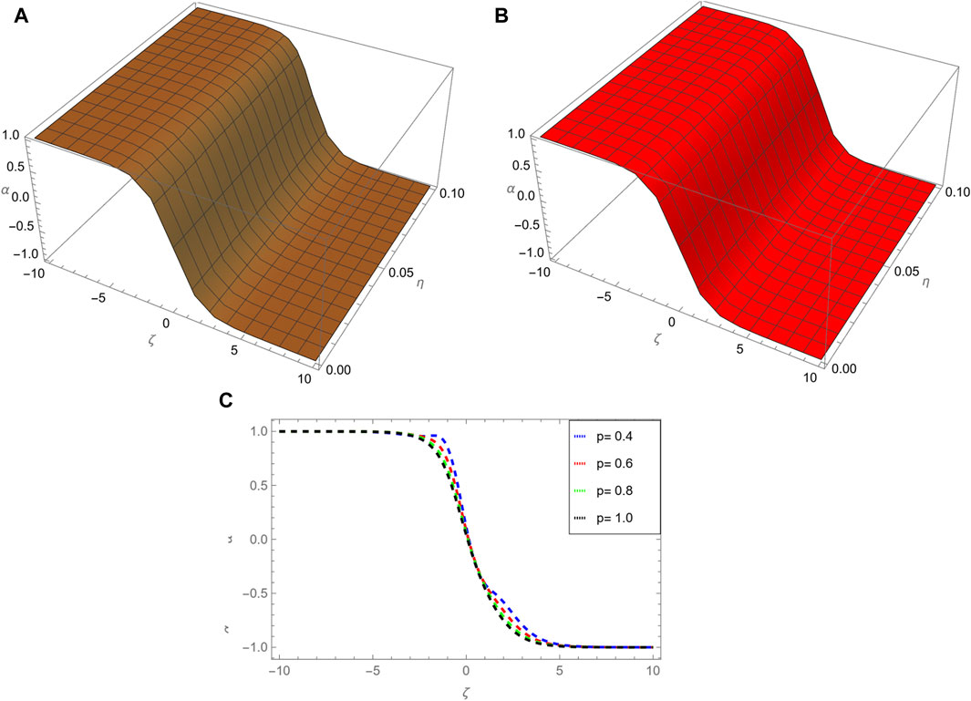
Figure 1. This figure shows, (A) the ARPSM solution for p = 1, (B) exact solution, (C) different fractional order comparison of α(ζ, η) for η = 0.1.

Figure 2

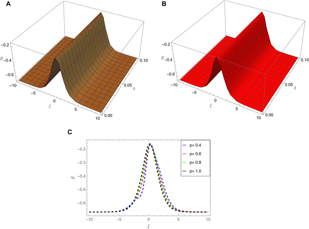
Figure 2. This figure demonstrates: (A) the ARPSM solution for p = 1, (B) exact solution, (C) different fractional order comparison of β(ζ, η) for η = 0.1.

Table 1

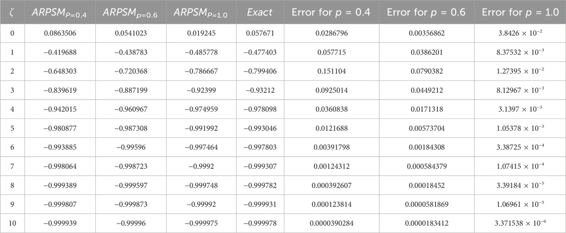
Table 1. The ARPSM fractional solution for various order of p for η = 0.1 of problem 1 α(ζ, η).

Table 2

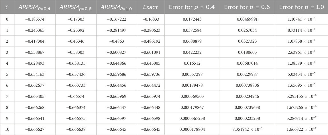
Table 2. The ARPSM fractional solution for various order of p for η =0.1 of problem 1 β(ζ, η).

3.3 Problem 2

Examine the system of homogeneous Burger’s equations as follows:

\begin{aligned} D_{η}^{p} α (ζ, η) - \frac{\partial^{2} α (ζ, η)}{\partial ζ^{2}} - 2 α (ζ, η) \frac{\partial α (ζ, η)}{\partial ζ} + β (ζ, η) \frac{\partial α (ζ, η)}{\partial ζ} + α (ζ, η) \frac{\partial β (ζ, η)}{\partial ζ} = 0, \end{aligned} (63)

\begin{aligned} D_{η}^{p} β (ζ, η) - \frac{\partial^{2} β (ζ, η)}{\partial ζ^{2}} - 2 β (ζ, η) \frac{\partial β (ζ, η)}{\partial ζ} + β (ζ, η) \frac{\partial α (ζ, η)}{\partial ζ} + α (ζ, η) \frac{\partial β (ζ, η)}{\partial ζ} = 0, \\ where 0 < p \leq 1 \end{aligned} (64)

with the following initial conditions:

\begin{aligned} α (ζ, 0) = c o s (ζ), \end{aligned} (65)

\begin{aligned} β (ζ, 0) = c o s (ζ), \end{aligned} (66)

and exact solution

\begin{aligned} α (ζ, η) = e^{- η} \cos (ζ), \end{aligned} (67)

\begin{aligned} β (ζ, η) = e^{- η} \cos (ζ) . \end{aligned} (68)

By applying Eqs 65, 66 and the AT on Eqs 63, 64, we are able to derive:

\begin{aligned} α (ζ, s) - \frac{c o s (ζ)}{s^{2}} - \frac{1}{s^{p}} [\frac{\partial^{2} α (ζ, s)}{\partial ζ^{2}}] - \frac{2}{s^{p}} A_{η} [A_{η}^{- 1} α (ζ, s) \frac{\partial A_{η}^{- 1} α (ζ, s)}{\partial ζ}] \\ + \frac{1}{s^{p}} A_{η} [A_{η}^{- 1} β (ζ, s) \frac{\partial A_{η}^{- 1} α (ζ, s)}{\partial ζ}] + \frac{1}{s^{p}} A_{η} [A_{η}^{- 1} α (ζ, s) \frac{\partial A_{η}^{- 1} β (ζ, s)}{\partial ζ}] = 0, \end{aligned} (69)

\begin{aligned} β (ζ, s) - \frac{c o s (ζ)}{s^{2}} - \frac{1}{s^{p}} [\frac{\partial^{2} β (ζ, s)}{\partial ζ^{2}}] - \frac{2}{s^{p}} A_{η} [A_{η}^{- 1} β (ζ, s) \frac{\partial A_{η}^{- 1} β (ζ, s)}{\partial ζ}] \\ + \frac{1}{s^{p}} A_{η} [A_{η}^{- 1} β (ζ, s) \frac{\partial A_{η}^{- 1} α (ζ, s)}{\partial ζ}] + \frac{1}{s^{p}} A_{η} [A_{η}^{- 1} α (ζ, s) \frac{\partial A_{η}^{- 1} β (ζ, s)}{\partial ζ}] = 0, \end{aligned} (70)

As a result, the following term series have been kth truncated:

\begin{aligned} α (ζ, s) = \frac{\cos (ζ)}{s^{2}} + \sum_{r = 1}^{k} \frac{f_{r} (ζ, s)}{s^{r p + 1}}, r = 1,2,3,4 \dots . \end{aligned} (71)

\begin{aligned} β (ζ, s) = \frac{\cos (ζ)}{s^{2}} + \sum_{r = 1}^{k} \frac{g_{r} (ζ, s)}{s^{r p + 1}}, r = 1,2,3,4 \dots . \end{aligned} (72)

The residual function are

\begin{aligned} A_{η} R e s (ζ, s) = α (ζ, s) - \frac{c o s (ζ)}{s^{2}} - \frac{1}{s^{p}} [\frac{\partial^{2} α (ζ, s)}{\partial ζ^{2}}] - \frac{1}{s^{p}} A_{η} [A_{η}^{- 1} α (ζ, s) \frac{\partial A_{η}^{- 1} α (ζ, s)}{\partial ζ}] \\ + \frac{1}{s^{p}} A_{η} [A_{η}^{- 1} β (ζ, s) \frac{\partial A_{η}^{- 1} α (ζ, s)}{\partial ζ}] + \frac{1}{s^{p}} A_{η} [A_{η}^{- 1} α (ζ, s) \frac{\partial A_{η}^{- 1} β (ζ, s)}{\partial ζ}] = 0, \end{aligned} (73)

\begin{aligned} A_{η} R e s (ζ, s) = β (ζ, η) - \frac{c o s (ζ)}{s^{2}} - \frac{1}{s^{p}} [\frac{\partial^{2} β (ζ, s)}{\partial ζ^{2}}] - \frac{2}{s^{p}} A_{η} [A_{η}^{- 1} β (ζ, s) \frac{\partial A_{η}^{- 1} β (ζ, s)}{\partial ζ}] \\ + \frac{1}{s^{p}} A_{η} [A_{η}^{- 1} β (ζ, s) \frac{\partial A_{η}^{- 1} α (ζ, s)}{\partial ζ}] + \frac{1}{s^{p}} A_{η} [A_{η}^{- 1} α (ζ, s) \frac{\partial A_{η}^{- 1} β (ζ, s)}{\partial ζ}] = 0, \end{aligned} (74)

and the kth-LRFs as:

\begin{aligned} A_{η} R e s_{k} (ζ, s) = α_{k} (ζ, s) - \frac{c o s (ζ)}{s^{2}} - \frac{1}{s^{p}} [\frac{\partial^{2} α_{k} (ζ, s)}{\partial ζ^{2}}] - \frac{1}{s^{p}} A_{η} [A_{η}^{- 1} α_{k} (ζ, s) \frac{\partial A_{η}^{- 1} α_{k} (ζ, s)}{\partial ζ}] \\ + \frac{1}{s^{p}} A_{η} [A_{η}^{- 1} β_{k} (ζ, s) \frac{\partial A_{η}^{- 1} α_{k} (ζ, s)}{\partial ζ}] + \frac{1}{s^{p}} A_{η} [A_{η}^{- 1} α_{k} (ζ, s) \frac{\partial A_{η}^{- 1} β_{k} (ζ, s)}{\partial ζ}] = 0, \end{aligned} (75)

\begin{aligned} A_{η} R e s_{k} (ζ, s) = β_{k} (ζ, s) - \frac{c o s (ζ)}{s^{2}} - \frac{1}{s^{p}} [\frac{\partial^{2} β_{k} (ζ, s)}{\partial ζ^{2}}] - \frac{1}{s^{p}} A_{η} [A_{η}^{- 1} β_{k} (ζ, s) \frac{\partial A_{η}^{- 1} β_{k} (ζ, s)}{\partial ζ}] \\ + \frac{1}{s^{p}} A_{η} [A_{η}^{- 1} β_{k} (ζ, s) \frac{\partial A_{η}^{- 1} α_{k} (ζ, s)}{\partial ζ}] + \frac{1}{s^{p}} A_{η} [A_{η}^{- 1} α_{k} (ζ, s) \frac{\partial A_{η}^{- 1} β_{k} (ζ, s)}{\partial ζ}] = 0, \end{aligned} (76)

To obtain f_r(ζ, s) and g_r(ζ, s), do the following procedures: The rth-truncated series from Eqs 71, 72 should be substituted into the rth-Aboodh residual function depicted in Eqs 75, 76, and the resultant equations should be multiplied by s^rp+1. The relations lim_s→∞(s^rp+1AηResα, r(ζ, s)) = 0 and lim_s→∞(s^rp+1AηResβ, r(ζ, s)) = 0 are then solved iteratively.in the case of r = 1, 2, 3, ⋯. Listed below are the first few terms:

\begin{aligned} f_{1} (ζ, s) = - \cos (ζ), \\ g_{1} (ζ, s) = - \cos (ζ), \end{aligned} (77)

\begin{aligned} f_{2} (ζ, s) = \cos (ζ), \\ g_{2} (ζ, s) = \cos (ζ) . \end{aligned} (78)

\begin{aligned} f_{2} (ζ, s) = - \cos (ζ), \\ g_{2} (ζ, s) = - \cos (ζ) . \end{aligned} (79)

and so on.For each r = 1, 2, 3, … , we put the values of f_r(ζ, s) and g_r(ζ, s) in Eqs 71 and 72, and obtain

\begin{aligned} α (ζ, s) = - \frac{\cos (ζ)}{s^{p + 1}} + \frac{\cos (ζ)}{s^{2 p + 1}} - \frac{\cos (ζ)}{s^{3 p + 1}} + \frac{\cos (ζ)}{s} + \dots . \end{aligned} (80)

\begin{aligned} β (ζ, s) = - \frac{\cos (ζ)}{s^{p + 1}} + \frac{\cos (ζ)}{s^{2 p + 1}} - \frac{\cos (ζ)}{s^{3 p + 1}} + \frac{\cos (ζ)}{s} + \dots . \end{aligned} (81)

Utilizing the inverse transform of Aboodh, we get

\begin{aligned} α (ζ, η) = \cos (ζ) + \frac{\cos (ζ) η^{2 p}}{Γ (2 p + 1)} - \frac{\cos (ζ) η^{3 p}}{Γ (3 p + 1)} - \frac{\cos (ζ) η^{p}}{Γ (p + 1)} + \dots . \end{aligned} (82)

\begin{aligned} β (ζ, η) = \cos (ζ) + \frac{\cos (ζ) η^{2 p}}{Γ (2 p + 1)} - \frac{\cos (ζ) η^{3 p}}{Γ (3 p + 1)} - \frac{\cos (ζ) η^{p}}{Γ (p + 1)} + \dots . \end{aligned} (83)

Figures 3A–C show comparative analysis of different fractional order p = 0.4, 0.6, 1.0 for α, β(ζ, η) at η = 0.1 respectively. The different fractional order graphs of two and three dimensional of problem 2 are introduced in Figure 4. In Table 3, we introduce an analysis for the ARPSM fractional solution for various p for η = 0.1 of problem 2 α(ζ, η) and β(ζ, η).

Figure 3

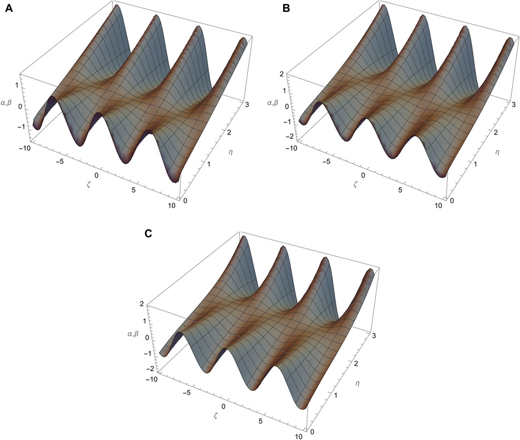
Figure 3. (A–C) show comparative analysis of different fractional order p = 0.4, 0.6, 1.0 for α, β(ζ, η) at η = 0.1, respectively.

Figure 4

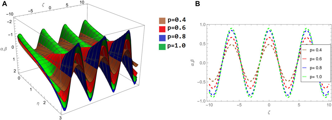
Figure 4. Comparative analysis of fractional order p in (A) 3D graph and (B) 2D graph.

Table 3

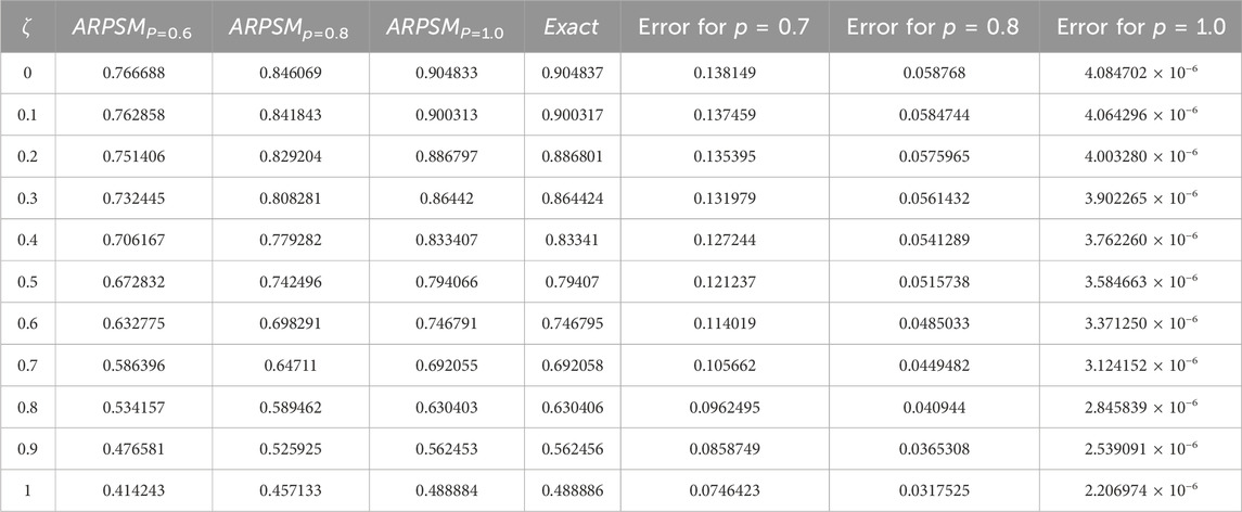
Table 3. The ARPSM fractional solution for various p for η =0.1 of problem 2 α(ζ, η) and β(ζ, η).

3.4 The Aboodh iterative transform Method’s concept

Our focus will be on a general space-time PDE of fractional order.

D_{η}^{p} α (ζ, η) = Φ (α (ζ, η), D_{ζ}^{η} α (ζ, η), D_{ζ}^{2 η} α (ζ, η), D_{ζ}^{3 η} α (ζ, η)), 0 < p, η \leq 1, (84)

With the following initial conditions:

α^{(k)} (ζ, 0) = h_{k}, k = 0,1,2, \dots, m - 1, (85)

Let $Φ (α (ζ, η), D_{ζ}^{η} α (ζ, η), D_{ζ}^{2 η} α (ζ, η), D_{ζ}^{3 η} α (ζ, η))$ be a nonlinear or linear operator of $α (ζ, η) D_{ζ}^{η} α (ζ, η), D_{ζ}^{2 η} α (ζ, η)$ and $D_{ζ}^{3 η} α (ζ, η)$ , and let α(ζ, η) be the assumed unknown function. The AT is applied to both sides of Eq. 84 to provide the following equation. α is used instead of α(ζ, η) for simplicity.

A [α (ζ, η)] = \frac{1}{s^{p}} (\sum_{k = 0}^{m - 1} \frac{α^{(k)} (ζ, 0)}{s^{2 - p + k}} + A [Φ (α (ζ, η), D_{ζ}^{η} α (ζ, η), D_{ζ}^{2 η} α (ζ, η), D_{ζ}^{3 η} α (ζ, η))]), (86)

Aboodh inverse transform gives:

α (ζ, η) = A^{- 1} [\frac{1}{s^{p}} (\sum_{k = 0}^{m - 1} \frac{α^{(k)} (ζ, 0)}{s^{2 - p + k}} + A [Φ (α (ζ, η), D_{ζ}^{η} α (ζ, η), {\times D}_{ζ}^{2 η} α (ζ, η), D_{ζ}^{3 η} α (ζ, η))]) . (87)

The solution through this method is represented as an infinite series.

α (ζ, η) = \sum_{i = 0}^{\infty} α_{i} . (88)

Since $Φ (α, D_{ζ}^{η} α, D_{ζ}^{2 η} α, D_{ζ}^{3 η} α)$ is either a nonlinear or linear operator which can be decomposed as follows:

\begin{aligned} Φ (α, D_{ζ}^{η} α, D_{ζ}^{2 η} α, D_{ζ}^{3 η} α) = Φ (α_{0}, D_{ζ}^{η} α_{0}, D_{ζ}^{2 η} α_{0}, D_{ζ}^{3 η} α_{0}) \\ + \sum_{i = 0}^{\infty} (Φ (\sum_{k = 0}^{i} (α_{k}, D_{ζ}^{η} α_{k}, D_{ζ}^{2 η} α_{k}, D_{ζ}^{3 η} α_{k})) - Φ (\sum_{k = 1}^{i - 1} (α_{k}, D_{ζ}^{η} α_{k}, D_{ζ}^{2 η} α_{k}, D_{ζ}^{3 η} α_{k})))) . \end{aligned} (89)

Eqs 88, 89 must be substituted into Eq. 87 in order to get the subsequent equation.

\begin{aligned} \sum_{i = 0}^{\infty} α_{i} (ζ, η) = A^{- 1} [\frac{1}{s^{p}} (\sum_{k = 0}^{m - 1} \frac{α^{(k)} (ζ, 0)}{s^{2 - p + k}} + A [Φ (α_{0}, D_{ζ}^{η} α_{0}, D_{ζ}^{2 η} α_{0}, D_{ζ}^{3 η} α_{0})])] \\ + A^{- 1} [\frac{1}{s^{p}} (A [\sum_{i = 0}^{\infty} (Φ \sum_{k = 0}^{i} (α_{k}, D_{ζ}^{η} α_{k}, D_{ζ}^{2 η} α_{k}, D_{ζ}^{3 η} α_{k}))])] \\ - A^{- 1} [\frac{1}{s^{p}} (A [(Φ \sum_{k = 1}^{i - 1} (α_{k}, D_{ζ}^{η} α_{k}, D_{ζ}^{2 η} α_{k}, D_{ζ}^{3 η} α_{k}))])] \end{aligned} (90)

\begin{aligned} α_{0} (ζ, η) = A^{- 1} [\frac{1}{s^{p}} (\sum_{k = 0}^{m - 1} \frac{α^{(k)} (ζ, 0)}{s^{2 - p + k}})], \\ α_{1} (ζ, η) = A^{- 1} [\frac{1}{s^{p}} (A [Φ (α_{0}, D_{ζ}^{η} α_{0}, D_{ζ}^{2 η} α_{0}, D_{ζ}^{3 η} α_{0})])], \\ ⋮ \\ α_{m + 1} (ζ, η) = A^{- 1} [\frac{1}{s^{p}} (A [\sum_{i = 0}^{\infty} (Φ \sum_{k = 0}^{i} (α_{k}, D_{ζ}^{η} α_{k}, D_{ζ}^{2 η} α_{k}, D_{ζ}^{3 η} α_{k}))])] \\ - A^{- 1} [\frac{1}{s^{p}} (A [(Φ \sum_{k = 1}^{i - 1} (α_{k}, D_{ζ}^{η} α_{k}, D_{ζ}^{2 η} α_{k}, D_{ζ}^{3 η} α_{k}))])], m = 1,2, \dots . \end{aligned} (91)

The m-terms approximate solution to Eq. 84 is given as:

α (ζ, η) = \sum_{i = 0}^{m - 1} α_{i} . (92)

3.4.1 Solution of the problem via NITM

3.4.1.1 Problem 1

\begin{aligned} D_{η}^{p} α (ζ, η) = \frac{\partial^{3} α (ζ, η)}{\partial ζ^{3}} + 2 β (ζ, η) \frac{\partial α (ζ, η)}{\partial ζ} + α (ζ, η) \frac{\partial β (ζ, η)}{\partial ζ}, \end{aligned} (93)

\begin{aligned} D_{η}^{p} β (ζ, η) = α (ζ, η) \frac{\partial α (ζ, η)}{\partial ζ}, where 0 < p \leq 1 \end{aligned} (94)

with the following initial conditions:

\begin{aligned} α (ζ, 0) = - \tanh (\frac{ζ}{\sqrt{3}}) . \end{aligned} (95)

\begin{aligned} β (ζ, 0) = - \frac{1}{2} \tanh^{2} (\frac{ζ}{\sqrt{3}}) - \frac{1}{6} . \end{aligned} (96)

Both sides of Eqs 93, 94 is evaluated using AT, the following equations are produced as a result:

\begin{aligned} A [D_{η}^{p} α (ζ, η)] = \frac{1}{s^{p}} (\sum_{k = 0}^{m - 1} \frac{α^{(k)} (ζ, 0)}{s^{2 - p + k}} + A [\frac{\partial^{3} α (ζ, η)}{\partial ζ^{3}} + 2 β (ζ, η) \frac{\partial α (ζ, η)}{\partial ζ} + α (ζ, η) \frac{\partial β (ζ, η)}{\partial ζ}]) \end{aligned} (97)

\begin{aligned} A [D_{η}^{p} β (ζ, η)] = \frac{1}{s^{p}} (\sum_{k = 0}^{m - 1} \frac{β^{(k)} (ζ, 0)}{s^{2 - p + k}} + A [α (ζ, η) \frac{\partial α (ζ, η)}{\partial ζ}]) \end{aligned} (98)

For Eqs 97, 98, the application of the inverse AT results in the following equations:

\begin{aligned} α (ζ, η) = A^{- 1} [\frac{1}{s^{p}} (\sum_{k = 0}^{m - 1} \frac{α^{(k)} (ζ, 0)}{s^{2 - p + k}} + A [\frac{\partial^{3} α (ζ, η)}{\partial ζ^{3}} + 2 β (ζ, η) \frac{\partial α (ζ, η)}{\partial ζ} + α (ζ, η) \frac{\partial β (ζ, η)}{\partial ζ}])] \end{aligned} (99)

\begin{aligned} β (ζ, η) = A^{- 1} [\frac{1}{s^{p}} (\sum_{k = 0}^{m - 1} \frac{β^{(k)} (ζ, 0)}{s^{2 - p + k}} + A [α (ζ, η) \frac{\partial α (ζ, η)}{\partial ζ}])] \end{aligned} (100)

Utilizing the AT in an iterative manner results in the extraction of the following equation:

\begin{aligned} α_{0} (ζ, η) = A^{- 1} [\frac{1}{s^{p}} (\sum_{k = 0}^{m - 1} \frac{α^{(k)} (ζ, 0)}{s^{2 - p + k}})] \\ = A^{- 1} [\frac{α (ζ, 0)}{s^{2}}] \\ = - \tanh (\frac{ζ}{\sqrt{3}}), \end{aligned}

\begin{aligned} β_{0} (ζ, η) = A^{- 1} [\frac{1}{s^{p}} (\sum_{k = 0}^{m - 1} \frac{β^{(k)} (ζ, 0)}{s^{2 - p + k}})] \\ = A^{- 1} [\frac{β (ζ, 0)}{s^{2}}] \\ = - \frac{1}{2} \tanh^{2} (\frac{ζ}{\sqrt{3}}) - \frac{1}{6}, \end{aligned}

By applying the RL integral to Eqs 93, 94, we perform the objective of obtaining the equivalent form.

\begin{aligned} α (ζ, η) = - \tanh (\frac{ζ}{\sqrt{3}}) + A [\frac{\partial^{3} α (ζ, η)}{\partial ζ^{3}} + 2 β (ζ, η) \frac{\partial α (ζ, η)}{\partial ζ} + α (ζ, η) \frac{\partial β (ζ, η)}{\partial ζ}] \end{aligned} (101)

\begin{aligned} β (ζ, η) = - \frac{1}{2} \tanh^{2} (\frac{ζ}{\sqrt{3}}) - \frac{1}{6} + A [α (ζ, η) \frac{\partial α (ζ, η)}{\partial ζ}] \end{aligned} (102)

The following few terms are produced by the NITM method.

\begin{aligned} α_{0} (ζ, η) = - \tanh (\frac{ζ}{\sqrt{3}}), \\ β_{0} (ζ, η) = - \frac{1}{2} \tanh^{2} (\frac{ζ}{\sqrt{3}}) - \frac{1}{6}, \\ α_{1} (ζ, η) = \frac{{sech}^{2} (\frac{ζ}{\sqrt{3}}) η^{p}}{\sqrt{3} Γ (p + 1)}, \\ β_{1} (ζ, η) = \frac{\tanh (\frac{ζ}{\sqrt{3}}) {sech}^{2} (\frac{ζ}{\sqrt{3}}) η^{p}}{\sqrt{3} Γ (p + 1)}, \\ α_{2} (ζ, η) = \frac{1}{9} {sech}^{4} (\frac{ζ}{\sqrt{3}}) η^{2 p} (\frac{\sqrt{\frac{3}{π}} 4^{p} (7 {sech}^{2} (\frac{ζ}{\sqrt{3}}) - 6) η^{p} Γ (p + \frac{1}{2})}{Γ (p + 1) Γ (3 p + 1)} + \frac{3 \cosh (\frac{2 ζ}{\sqrt{3}})}{Γ (2 p + 1)}), \\ β_{2} (ζ, η) = \frac{1}{18} {sech}^{5} (\frac{ζ}{\sqrt{3}}) η^{2 p} \times (\frac{3 (\cosh (\sqrt{3} ζ) - 3 \cosh (\frac{ζ}{\sqrt{3}}))}{Γ (2 p + 1)} - \frac{\sqrt{\frac{3}{π}} 4^{p + 1} \cosh (\frac{ζ}{\sqrt{3}}) η^{p} Γ (p + \frac{1}{2})}{Γ (p + 1) Γ (3 p + 1)}) . \end{aligned} (103)

The final solution through NITM algorithm is presented in the following manner:

\begin{aligned} α (ζ, η) = α_{0} (ζ, η) + α_{1} (ζ, η) + α_{2} (ζ, η) + \dots . \end{aligned} (104)

\begin{aligned} β (ζ, η) = β_{0} (ζ, η) + β_{1} (ζ, η) + β_{2} (ζ, η) + \dots . \end{aligned} (105)

\begin{aligned} v (ζ, t) = - \tanh (\frac{ζ}{\sqrt{3}}) + \frac{{sech}^{2} (\frac{ζ}{\sqrt{3}}) η^{p}}{\sqrt{3} Γ (p + 1)} \\ + \frac{1}{9} {sech}^{4} (\frac{ζ}{\sqrt{3}}) η^{2 p} (\frac{\sqrt{\frac{3}{π}} 4^{p} (7 {sech}^{2} (\frac{ζ}{\sqrt{3}}) - 6) η^{p} Γ (p + \frac{1}{2})}{Γ (p + 1) Γ (3 p + 1)} + \frac{3 \cosh (\frac{2 ζ}{\sqrt{3}})}{Γ (2 p + 1)}) + \dots . \end{aligned} (106)

\begin{aligned} w (ζ, t) = - \frac{1}{2} \tanh^{2} (\frac{ζ}{\sqrt{3}}) - \frac{1}{6} + \frac{\tanh (\frac{ζ}{\sqrt{3}}) {sech}^{2} (\frac{ζ}{\sqrt{3}}) η^{p}}{\sqrt{3} Γ (p + 1)} \\ + \frac{1}{18} {sech}^{5} (\frac{ζ}{\sqrt{3}}) η^{2 p} (\frac{3 (\cosh (\sqrt{3} ζ) - 3 \cosh (\frac{ζ}{\sqrt{3}}))}{Γ (2 p + 1)} - \frac{\sqrt{\frac{3}{π}} 4^{p + 1} \cosh (\frac{ζ}{\sqrt{3}}) η^{p} Γ (p + \frac{1}{2})}{Γ (p + 1) Γ (3 p + 1)}) + \dots . \end{aligned} (107)

Figure 5 illustrates, (a) the NITM solution for p = 1, (b) exact solution, (c) different fractional order comparison of α(ζ, η) for η = 0.1. Figure 6 demonstrates, (a) the NITM solution for p = 1, (b) exact solution, (c) different fractional order comparison of β(ζ, η) for η = 0.1. In Table 4 the NITM fractional solution for various order p for η = 0.1 of problem 1 is analyzed. In Table 5, the NITM fractional solution for various order p for η = 0.1 of problem 1 is analyzed.

Figure 5

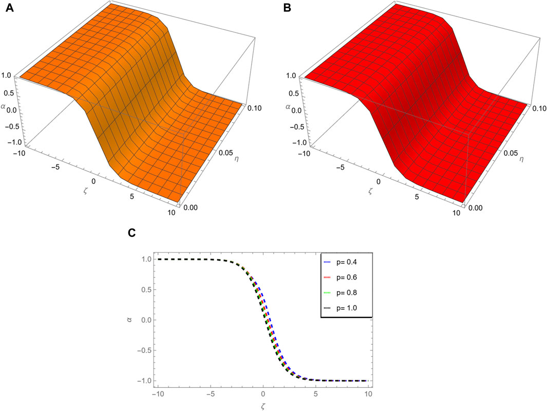
Figure 5. In figure, (A) shows NITM solution for p = 1, (B) shows exact solution, (C) shows different fractional order comparison of α(ζ, η) for η = 0.1.

Figure 6

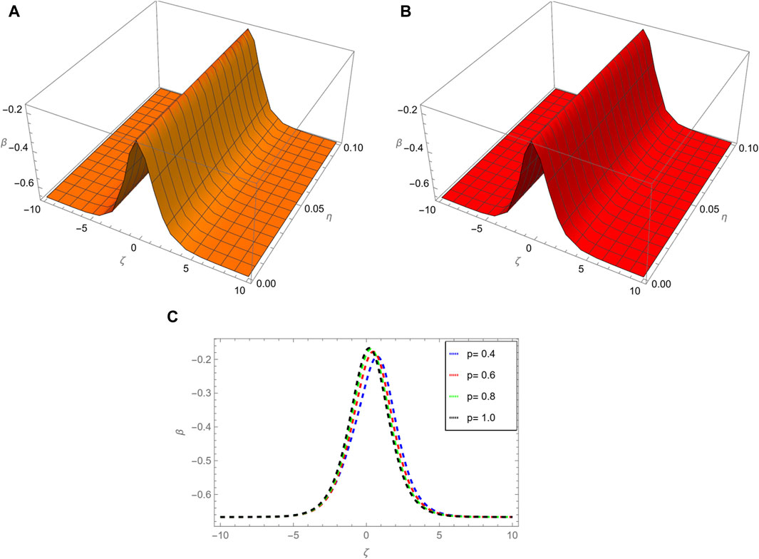
Figure 6. In figure, (A) shows NITM solution for p = 1, (B) shows exact solution, (C) shows different fractional order comparison of β(ζ, η) for η = 0.1.

Table 4

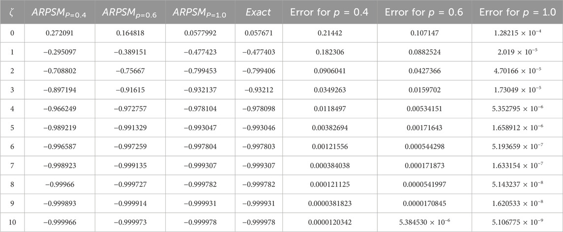
Table 4. The NITM fractional solution for various order p for η = 0.1 of problem 1 α(ζ, η).

Table 5

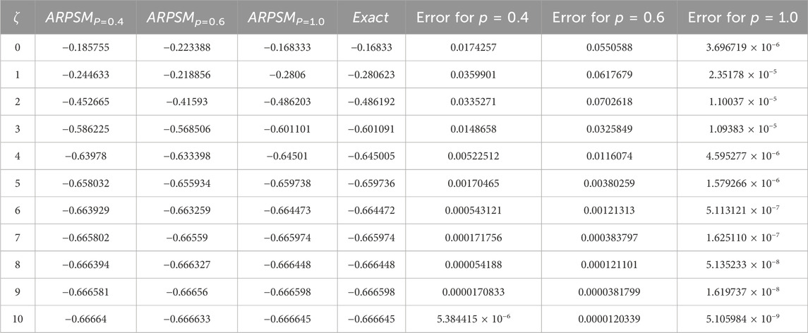
Table 5. The NITM fractional solution for various order p for η = 0.1 of problem 1 β(ζ, η).

3.4.1.2 Problem 2

\begin{aligned} D_{η}^{p} α (ζ, η) = \frac{\partial^{2} α (ζ, η)}{\partial ζ^{2}} + 2 α (ζ, η) \frac{\partial α (ζ, η)}{\partial ζ} - β (ζ, η) \frac{\partial α (ζ, η)}{\partial ζ} - α (ζ, η) \frac{\partial β (ζ, η)}{\partial ζ}, \end{aligned} (108)

\begin{aligned} D_{η}^{p} β (ζ, η) = \frac{\partial^{2} β (ζ, η)}{\partial ζ^{2}} + 2 β (ζ, η) \frac{\partial β (ζ, η)}{\partial ζ} - β (ζ, η) \frac{\partial α (ζ, η)}{\partial ζ} - α (ζ, η) \frac{\partial β (ζ, η)}{\partial ζ}, \\ where 0 < p \leq 1 \end{aligned} (109)

with the following initial conditions:

\begin{aligned} α (ζ, 0) = \cos (ζ), \end{aligned} (110)

\begin{aligned} β (ζ, 0) = \cos (ζ), \end{aligned} (111)

Both sides of Eqs 108, 109 is evaluated using AT, the following equations are produced as a result:

\begin{aligned} A [D_{η}^{p} α (ζ, η)] = \frac{1}{s^{p}} (\sum_{k = 0}^{m - 1} \frac{α^{(k)} (ζ, 0)}{s^{2 - p + k}} + A [\frac{\partial^{2} α (ζ, η)}{\partial ζ^{2}} + 2 α (ζ, η) \frac{\partial α (ζ, η)}{\partial ζ} - β (ζ, η) \frac{\partial α (ζ, η)}{\partial ζ} \\ - α (ζ, η) \frac{\partial β (ζ, η)}{\partial ζ}]) \end{aligned} (112)

\begin{aligned} A [D_{η}^{p} β (ζ, η)] = \frac{1}{s^{p}} (\sum_{k = 0}^{m - 1} \frac{β^{(k)} (ζ, 0)}{s^{2 - p + k}} + A [\frac{\partial^{2} β (ζ, η)}{\partial ζ^{2}} + 2 β (ζ, η) \frac{\partial β (ζ, η)}{\partial ζ} - β (ζ, η) \frac{\partial α (ζ, η)}{\partial ζ} \\ - α (ζ, η) \frac{\partial β (ζ, η)}{\partial ζ}]) \end{aligned} (113)

For Eqs 112, 113, the application of the inverse AT results in the following equations:

\begin{aligned} α (ζ, η) = A^{- 1} [\frac{1}{s^{p}} (\sum_{k = 0}^{m - 1} \frac{α^{(k)} (ζ, 0)}{s^{2 - p + k}} + A [\frac{\partial^{2} α (ζ, η)}{\partial ζ^{2}} + 2 α (ζ, η) \frac{\partial α (ζ, η)}{\partial ζ} - β (ζ, η) \frac{\partial α (ζ, η)}{\partial ζ} \\ - α (ζ, η) \frac{\partial β (ζ, η)}{\partial ζ}])] \end{aligned} (114)

\begin{aligned} β (ζ, η) = A^{- 1} [\frac{1}{s^{p}} (\sum_{k = 0}^{m - 1} \frac{β^{(k)} (ζ, 0)}{s^{2 - p + k}} + A [\frac{\partial^{2} β (ζ, η)}{\partial ζ^{2}} + 2 β (ζ, η) \frac{\partial β (ζ, η)}{\partial ζ} - β (ζ, η) \frac{\partial α (ζ, η)}{\partial ζ} \\ - α (ζ, η) \frac{\partial β (ζ, η)}{\partial ζ}])] \end{aligned} (115)

Utilizing the AT in an iterative manner results in the extraction of the following equation:

\begin{aligned} {(α)}_{0} (ζ, η) = A^{- 1} [\frac{1}{s^{p}} (\sum_{k = 0}^{m - 1} \frac{α^{(k)} (ζ, 0)}{s^{2 - p + k}})] \\ = A^{- 1} [\frac{α (ζ, 0)}{s^{2}}] \\ = \cos (ζ), \end{aligned}

\begin{aligned} {(β)}_{0} (ζ, η) = A^{- 1} [\frac{1}{s^{p}} (\sum_{k = 0}^{m - 1} \frac{β^{(k)} (ζ, 0)}{s^{2 - p + k}})] \\ = A^{- 1} [\frac{β (ζ, 0)}{s^{2}}] \\ = \cos (ζ), \end{aligned}

By applying the RL integral to Eqs 108, 109, we perform the objective of obtaining the equivalent form.

\begin{aligned} α (ζ, η) = \cos (ζ) + A [\frac{\partial^{2} α (ζ, η)}{\partial ζ^{2}} + 2 α (ζ, η) \frac{\partial α (ζ, η)}{\partial ζ} - β (ζ, η) \frac{\partial α (ζ, η)}{\partial ζ} - α (ζ, η) \frac{\partial β (ζ, η)}{\partial ζ}] \end{aligned} (116)

\begin{aligned} β (ζ, η) = \cos (ζ) + A [\frac{\partial^{2} β (ζ, η)}{\partial ζ^{2}} + 2 β (ζ, η) \frac{\partial β (ζ, η)}{\partial ζ} - β (ζ, η) \frac{\partial α (ζ, η)}{\partial ζ} - α (ζ, η) \frac{\partial β (ζ, η)}{\partial ζ}] \end{aligned} (117)

The following few terms are produced by the NITM method.

\begin{aligned} α_{0} (ζ, η) = \cos (ζ), \\ β_{0} (ζ, η) = \cos (ζ), \\ α_{1} (ζ, η) = - \frac{η^{p} \cos (ζ)}{Γ (p + 1)}, \\ β_{1} (ζ, η) = - \frac{η^{p} \cos (ζ)}{Γ (p + 1)}, \\ α_{2} (ζ, η) = \frac{η^{2 p} \cos (ζ)}{Γ (2 p + 1)}, \\ β_{2} (ζ, η) = \frac{η^{2 p} \cos (ζ)}{Γ (2 p + 1)} . \\ α_{3} (ζ, η) = - \frac{η^{3 p} \cos (ζ)}{Γ (3 p + 1)}, \\ β_{3} (ζ, η) = - \frac{η^{3 p} \cos (ζ)}{Γ (3 p + 1)} . \end{aligned} (118)

The final solution through NITM algorithm is presented in the following manner:

\begin{aligned} α (ζ, η) = α_{0} (ζ, η) + α_{1} (ζ, η) + α_{2} (ζ, η) + \dots . \end{aligned} (119)

\begin{aligned} β (ζ, η) = β_{0} (ζ, η) + β_{1} (ζ, η) + β_{2} (ζ, η) + \dots . \end{aligned} (120)

\begin{aligned} α (ζ, t) = \cos (ζ) + \frac{\cos (ζ) η^{2 p}}{Γ (2 p + 1)} - \frac{\cos (ζ) η^{3 p}}{Γ (3 p + 1)} - \frac{\cos (ζ) η^{p}}{Γ (p + 1)} + \dots . \end{aligned} (121)

\begin{aligned} β (ζ, t) = \cos (ζ) + \frac{\cos (ζ) η^{2 p}}{Γ (2 p + 1)} - \frac{\cos (ζ) η^{3 p}}{Γ (3 p + 1)} - \frac{\cos (ζ) η^{p}}{Γ (p + 1)} + \dots . \end{aligned} (122)

Figures 7A–C show comparative analysis of different fractional order p = 0.4, 0.6, 1.0 for α, β(ζ, η) at η = 0.1, respectively. The two and three dimensional graphs of different fractional order p of problem 2 are introduced in Figure 8. Table 6, the NITM fractional solution for various order of p for η = 0.1 of problem 2 α(ζ, η) and β(ζ, η). Table 7, comparative analysis of example 1 solution through NITM and ARPSM of α(ζ, η) for η = 0.1 and p = 1. Table 8, comparative analysis of example 1 solution through NITM and ARPSM of β(ζ, η) for η = 0.1 and p = 1. Table 9, comparative analysis of example 2 solution through NITM and ARPSM of α(ζ, η) and β(ζ, η) for η = 0.1 and p = 1.

Figure 7

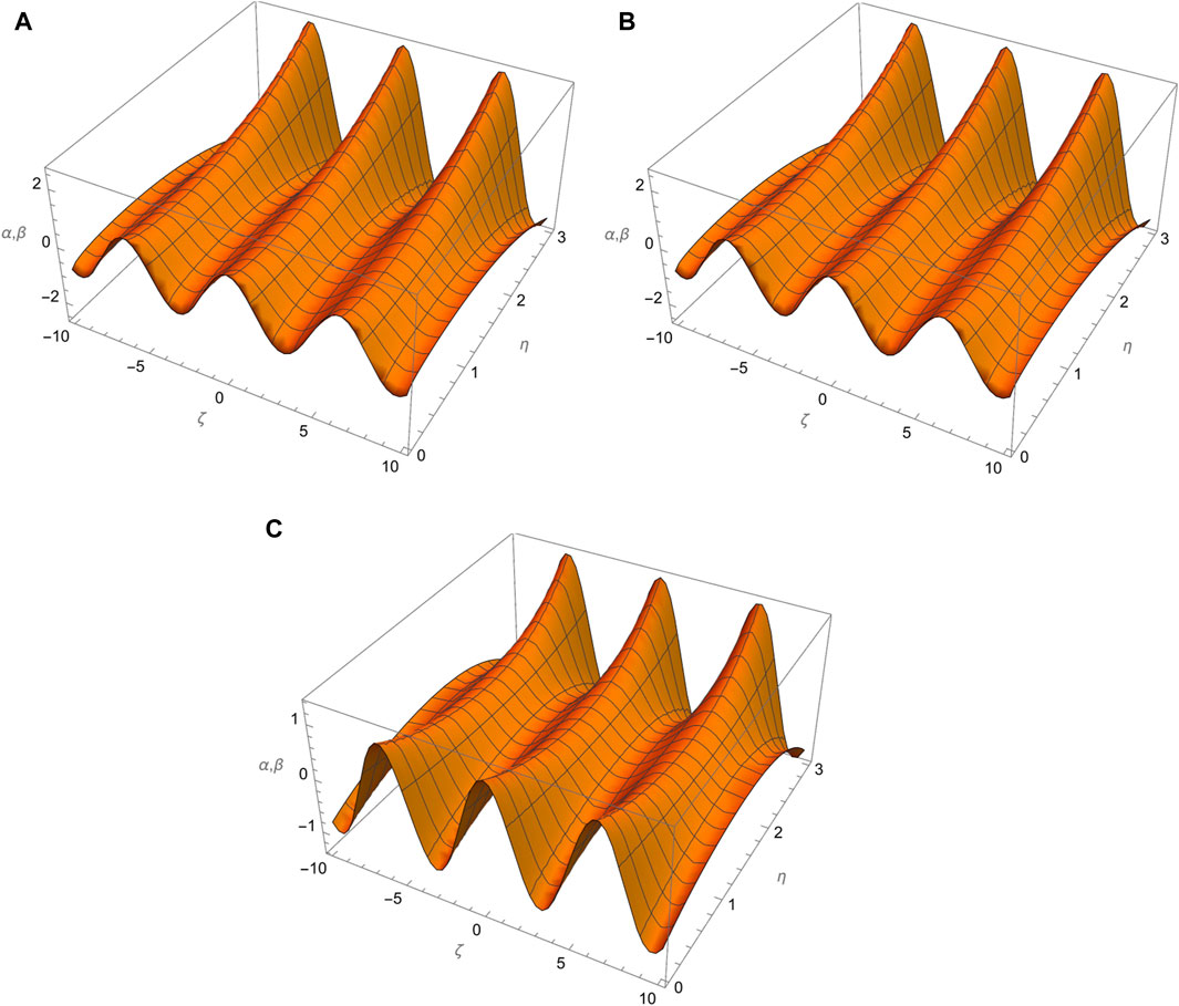
Figure 7. In figure, (A–C) shows comparative analysis of different fractional order p = 0.4, 0.6, 1.0 for α, β(ζ, η) at η = 0.1 respectively.

Figure 8

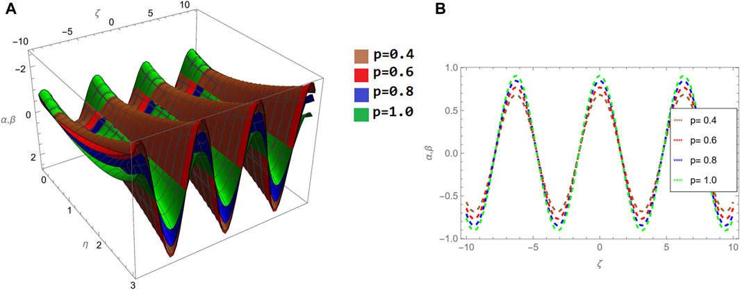
Figure 8. Comparative analysis of fractional order p in (A) 3D graph and (B) 2D graph.

Table 6

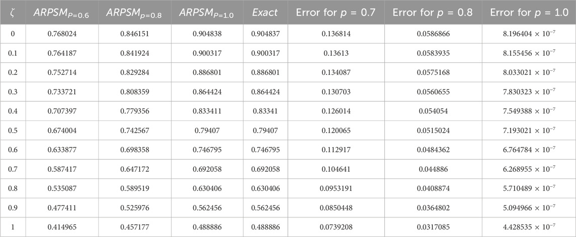
Table 6. The NITM fractional solution for various order of p for η = 0.1 of problem 2 α(ζ, η) and β(ζ, η).

Table 7

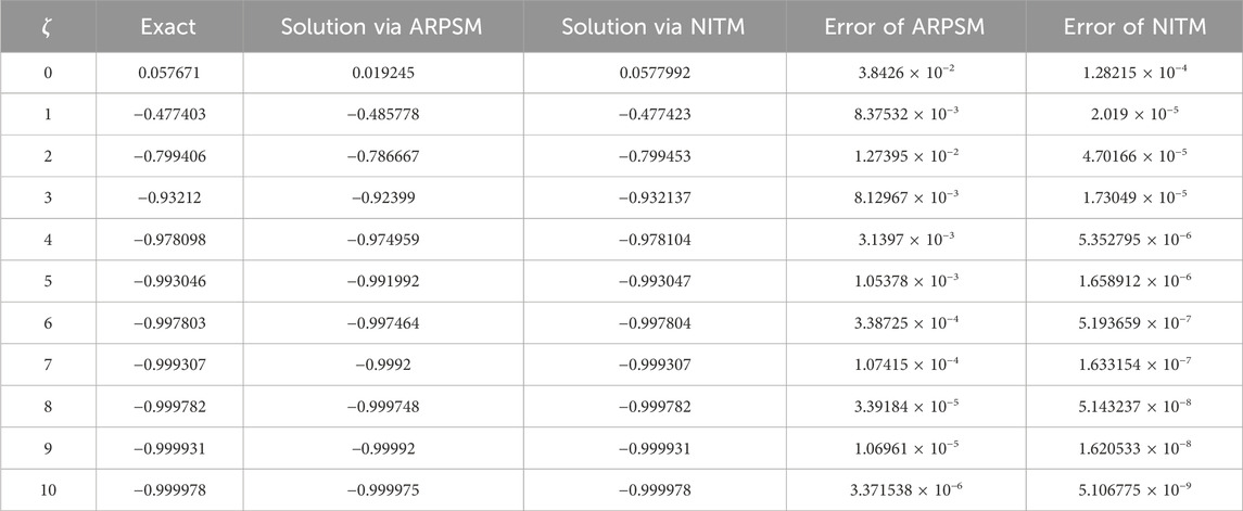
Table 7. Comparative analysis of example 1 solution through NITM and ARPSM of α(ζ, η) for η = 0.1 and p = 1.

Table 8

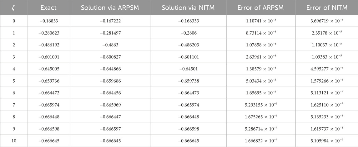
Table 8. Comparative analysis of example 1 solution through NITM and ARPSM of β(ζ, η) for η = 0.1 and p = 1.

Table 9

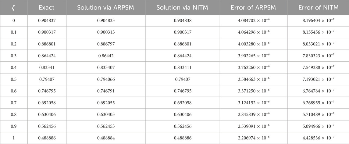
Table 9. Comparative analysis of example 2 solution through NITM and ARPSM of α(ζ, η) and β(ζ, η) for η = 0.1 and p = 1.

4 Conclusion

In conclusion, this study has examined the intricate dynamics of a system governed by nonlinear Korteweg-de Vries (KdV) equations and coupled Burger’s equations. Through the application of advanced mathematical tools, specifically the Aboodh transform iteration method (ATIM) and the Aboodh residual power series method (ARPSM), we have successfully obtained accurate solutions for this complex nonlinear system. The inclusion of the Caputo operator highlights the importance of fractional calculus in describing the system’s behavior. The results obtained through these methods contribute valuable insights into the understanding of the coupled equations’ dynamics. This research not only enhances our knowledge of mathematical modeling but also showcases the efficacy of the applied methods in analyzing intricate nonlinear systems. The findings pave the way for further exploration and applications in diverse scientific domains.

Future work: The methods used in this study can be utilized to investigate how the fractional parameter influences the characteristics of rogue waves and breathers in various plasma systems by solving a nonlinear Schrodinger equation and related evolution equations.

Data availability statement

The original contributions presented in the study are included in the article/supplementary material, further inquiries can be directed to the corresponding author.

Author contributions

SN: Formal Analysis, Investigation, Writing–original draft. WA: Software, Supervision, Validation, Writing–review and editing. RS: Conceptualization, Data curation, Methodology, Writing–review and editing. MA-S: Project administration, Supervision, Visualization, Software, Writing–review and editing. SI: Investigation, Project administration, Supervision, Visualization, Writing–review and editing.

Funding

The author(s) declare financial support was received for the research, authorship, and/or publication of this article. The authors express their gratitude to Princess Nourah bint Abdulrahman University Researchers Supporting Project Number (PNURSP2024R157), Princess Nourah bint Abdulrahman University, Riyadh, Saudi Arabia. This work was supported by the Deanship of Scientific Research, Vice Presidency for Graduate Studies and Scientific Research, King Faisal University, Saudi Arabia (Grant No. 5952).

Acknowledgments

The authors express their gratitude to Princess Nourah bint Abdulrahman University Researchers Supporting Project Number (PNURSP2024R157), Princess Nourah bint Abdulrahman University, Riyadh, Saudi Arabia. This work was supported by the Deanship of Scientific Research, Vice Presidency for Graduate Studies and Scientific Research, King Faisal University, Saudi Arabia (Grant No. 5952).

Conflict of interest

The authors declare that the research was conducted in the absence of any commercial or financial relationships that could be construed as a potential conflict of interest.

Publisher’s note

All claims expressed in this article are solely those of the authors and do not necessarily represent those of their affiliated organizations, or those of the publisher, the editors and the reviewers. Any product that may be evaluated in this article, or claim that may be made by its manufacturer, is not guaranteed or endorsed by the publisher.

References

1. Obeidat NA, Rawashdeh MS. On theories of natural decomposition method applied to system of nonlinear differential equations in fluid mechanics. Adv Mech Eng (2023) 15(1):168781322211498. doi:10.1177/16878132221149835

CrossRef Full Text | Google Scholar

2. Jafari H, Ganji RM, Ganji DD, Hammouch Z, Gasimov YS. A novel numerical method for solving fuzzy variable-order differential equations with Mittag-Leffler kernels. Fractals (2023) 31:2340063. doi:10.1142/s0218348x23400637

CrossRef Full Text | Google Scholar

3. Zhang L, Kwizera S, Khalique CM. A study of a new generalized burgers equations: symmetry soluions and conservation laws. Adv Math Models Appl (2023) 8(2).

Google Scholar

4. Srivastava HM, Iqbal J, Arif M, Khan A, Gasimov YS, Chinram R. A new application of Gauss quadrature method for solving systems of nonlinear equations. Symmetry (2021) 13(3):432. doi:10.3390/sym13030432

CrossRef Full Text | Google Scholar

5. Kai Y, Chen S, Zhang K, Yin Z. Exact solutions and dynamic properties of a nonlinear fourth-order time-fractional partial differential equation. Waves in Random and Complex Media (2022) 1–12. doi:10.1080/17455030.2022.2044541

CrossRef Full Text | Google Scholar

6. Cai X, Tang R, Zhou H, Li Q, Ma S, Wang D, et al. Dynamically controlling terahertz wavefronts with cascaded metasurfaces. Adv Photon (2021) 3(3):036003. doi:10.1117/1.AP.3.3.036003

CrossRef Full Text | Google Scholar

7. Yang R, Kai Y. Dynamical properties, modulation instability analysis and chaotic behaviors to the nonlinear coupled Schrodinger equation in fiber Bragg gratings. Mod Phys Lett B (2023) 38(06):2350239. doi:10.1142/S0217984923502391

CrossRef Full Text | Google Scholar

8. Zhou X, Liu X, Zhang G, Jia L, Wang X, Zhao Z. An iterative threshold algorithm of log-sum regularization for sparse problem. IEEE Trans Circuits Syst Video Technol (2023) 33(9):4728–40. doi:10.1109/TCSVT.2023.3247944

CrossRef Full Text | Google Scholar

9. Sierociuk D, Skovranek T, Macias M, Podlubny I, Petras I, Dzielinski A, et al. Diffusion process modeling by using fractional-order models. Appl Maths Comput (2015) 257:2–11. doi:10.1016/j.amc.2014.11.028

CrossRef Full Text | Google Scholar

10. Saad Alshehry A, Imran M, Khan A, Weera W. Fractional view analysis of kuramoto-sivashinsky equations with non-singular kernel operators. Symmetry (2022) 14(7):1463. doi:10.3390/sym14071463

CrossRef Full Text | Google Scholar

11. Al-Sawalha MM, Khan A, Ababneh OY, Botmart T. Fractional view analysis of Kersten-Krasil’shchik coupled KdV-mKdV systems with non-singular kernel derivatives. AIMS Math (2022) 7:18334–59. doi:10.3934/math.20221010

CrossRef Full Text | Google Scholar

12. Alderremy AA, Iqbal N, Aly S, Nonlaopon K. Fractional series solution construction for nonlinear fractional reaction-diffusion brusselator model utilizing Laplace residual power series. Symmetry (2022) 14(9):1944. doi:10.3390/sym14091944

CrossRef Full Text | Google Scholar

13. Yasmin H, Aljahdaly NH, Saeed AM, Shah R. Investigating symmetric soliton solutions for the fractional coupled konno-onno system using improved versions of a novel analytical technique. Mathematics (2023) 11(12):2686. doi:10.3390/math11122686

CrossRef Full Text | Google Scholar

14. Alshammari S, Al-Sawalha MM, Shah R. Approximate analytical methods for a fractional-order nonlinear system of Jaulent-Miodek equation with energy-dependent Schrodinger potential. Fractal and Fractional (2023) 7(2):140. doi:10.3390/fractalfract7020140

CrossRef Full Text | Google Scholar

15. Elsayed EM, Nonlaopon K. The analysis of the fractional-order Navier-Stokes equations by a novel approach. J Funct Spaces (2022) 2022:1–18. doi:10.1155/2022/8979447

CrossRef Full Text | Google Scholar

16. Podlubny I. Fractional-order systems and fractional-order controllers. Kosice: Institute of Experimental Physics, Slovak Academy of Sciences (1994). p. 1–18.

Google Scholar

17. Alshammari S, Moaddy K, Alshammari M, Alsheekhhussain Z, Yar M, Al-sawalha MM, et al. Analysis of solitary wave solutions in the fractional-order Kundu-Eckhaus system. Scientific Rep (2024) 14(1):3688. doi:10.1038/s41598-024-53330-7

CrossRef Full Text | Google Scholar

18. El-Tantawy SA, Matoog RT, Alrowaily AW, Ismaeel SM. On the shock wave approximation to fractional generalized Burger-Fisher equations using the residual power series transform method. Phys Fluids (2024) 36(2). doi:10.1063/5.0187127

CrossRef Full Text | Google Scholar

19. Jiang B, Zhao Y, Dong J, Hu J. Analysis of the influence of trust in opposing opinions: an inclusiveness-degree based Signed Deffuant-Weisbush model. Inf Fusion (2024) 104:102173. doi:10.1016/j.inffus.2023.102173

CrossRef Full Text | Google Scholar

20. Wang R, Feng Q, Ji J. The discrete convolution for fractional cosine-sine series and its application in convolution equations. AIMS Maths (2024) 9(2):2641–56. doi:10.3934/math.2024130

CrossRef Full Text | Google Scholar

21. Korteweg DJ, De Vries G. XLI. On the change of form of long waves advancing in a rectangular canal, and on a new type of long stationary waves. Phil Mag (1895) 5(39):422–43. doi:10.1080/14786449508620739

CrossRef Full Text | Google Scholar

22. Yasmin H, Alshehry AS, Ganie AH, Shafee A, Shah R. Noise effect on soliton phenomena in fractional stochastic Kraenkel-Manna-Merle system arising in ferromagnetic materials. Scientific Rep (2024) 14(1):1810. doi:10.1038/s41598-024-52211-3

CrossRef Full Text | Google Scholar

23. Wazwaz AM. New sets of solitary wave solutions to the KdV, mKdV, and the generalized KdV equations. Commun Nonlinear Sci Numer Simulation (2008) 13(2):331–9. doi:10.1016/j.cnsns.2006.03.013

CrossRef Full Text | Google Scholar

24. Ray SS. Soliton solutions for time fractional coupled modified KdV equations using new coupled fractional reduced differential transform method. J Math Chem (2013) 51(8):2214–29. doi:10.1007/s10910-013-0210-3

CrossRef Full Text | Google Scholar

25. Almutlak SA, Parveen S, Mahmood S, Qamar A, Alotaibi BM, El-Tantawy SA. On the propagation of cnoidal wave and overtaking collision of slow shear Alfvén solitons in low β − magnetized plasmas. Phys Fluids (2023) 35:075130. doi:10.1063/5.0158292

CrossRef Full Text | Google Scholar

26. Albalawi W, El-Tantawy SA, Salas AH. On the rogue wave solution in the framework of a Korteweg–de Vries equation. Results Phys (2021) 30:104847. doi:10.1016/j.rinp.2021.104847

CrossRef Full Text | Google Scholar

27. Hashmi T, Jahangir R, Masood W, Alotaibi BM, Ismaeel SME, El-Tantawy SA. Head-on collision of ion-acoustic (modified) Korteweg–de Vries solitons in Saturn’s magnetosphere plasmas with two temperature superthermal electrons. Phys Fluids (2023) 35:103104. doi:10.1063/5.0171220

CrossRef Full Text | Google Scholar

28. El-Tantawy SA. Nonlinear dynamics of soliton collisions in electronegative plasmas: the phase shifts of the planar KdV-and mkdV-soliton collisions. Chaos Solitons Fractals (2016) 93:162–8. doi:10.1016/j.chaos.2016.10.011

CrossRef Full Text | Google Scholar

29. Shan Tariq M, Masood W, Siddiq M, Asghar S, Alotaibi BM, Sherif ME, et al. Bäcklund transformation for analyzing a cylindrical Korteweg–de Vries equation and investigating multiple soliton solutions in a plasma. Phys Fluids (2023) 35:103105. doi:10.1063/5.0166075

CrossRef Full Text | Google Scholar

30. Ali I, Masood W, Rizvi H, Alrowaily AW, Ismaeel SME, El-Tantawy SA. Archipelagos, islands, necklaces, and other exotic structures in external force-driven chaotic dusty plasmas. Solitons and Fractals (2023) 175:113931. doi:10.1016/j.chaos.2023.113931

CrossRef Full Text | Google Scholar

31. Wazwaz A-M, Alhejaili W, El-Tantawy SA. Study on extensions of (modified) Korteweg–de Vries equations: painlevé integrability and multiple soliton solutions in fluid mediums. Phys Fluids (2023) 35:093110. doi:10.1063/5.0169733

CrossRef Full Text | Google Scholar

32. Arif K, Ehsan T, Masood W, Asghar S, Alyousef HA, Elsayed TF, et al. Quantitative and qualitative analyses of the mKdV equation and modeling nonlinear waves in plasma. Front Phys (2023) 11:194. doi:10.3389/fphy.2023.1118786

CrossRef Full Text | Google Scholar

33. Batool N, Masood W, Siddiq M, Alrowaily AW, Ismaeel SME, El-Tantawy SA. Hirota bilinear method and multi-soliton interaction of electrostatic waves driven by cubic nonlinearity in pair-ion-electron plasmas. Phys Fluids (2023) 35:033109. doi:10.1063/5.0142447

CrossRef Full Text | Google Scholar

34. Kashkari BS, El-Tantawy SA, Salas AH, El-Sherif LS. Homotopy perturbation method for studying dissipative nonplanar solitons in an electronegative complex plasma. Chaos Solitons Fractals (2020) 130:109457. doi:10.1016/j.chaos.2019.109457

CrossRef Full Text | Google Scholar

35. El-Tantawy SA, Wazwaz A-M. Anatomy of modified Korteweg–de Vries equation for studying the modulated envelope structures in non-Maxwellian dusty plasmas: freak waves and dark soliton collisions. Phy Plasmas (2018) 25:092105. doi:10.1063/1.5045247

CrossRef Full Text | Google Scholar

36. Albalawi W, El-Tantawy SA, Alkhateeb SA. The phase shift analysis of the colliding dissipative KdV solitons. J Ocean Eng Sci (2022) 7:521–7. doi:10.1016/j.joes.2021.09.021

CrossRef Full Text | Google Scholar

37. El-Tantawy SA. Rogue waves in electronegative space plasmas: the link between the family of the KdV equations and the nonlinear Schrödinger equation. Astrophys Space Sci (2016) 361:164. doi:10.1007/s10509-016-2754-8

CrossRef Full Text | Google Scholar

38. El-Tantawy SA, El-Awady EI, Schlickeiser R. Freak waves in a plasma having Cairns particles. Astrophys Space Sci (2015) 360:49. doi:10.1007/s10509-015-2562-6

CrossRef Full Text | Google Scholar

39. El-Tantawy SA, Wazwaz A-M, Schlickeiser R. Solitons collision and freak waves in a plasma with Cairns-Tsallis particle distributions. Plasma Phys Control Fusion (2015) 57:125012. doi:10.1088/0741-3335/57/12/125012

CrossRef Full Text | Google Scholar

40. El-Tantawy SA, El-Awady EI, Tribeche M. On the rogue waves propagation in non-Maxwellian complex space plasmas. Phys Plasmas (2015) 22:113705. doi:10.1063/1.4935916

CrossRef Full Text | Google Scholar

41. El-Tantawy SA, Moslem WM. Nonlinear structures of the Korteweg-de Vries and modified Korteweg-de Vries equations in non-Maxwellian electron-positron-ion plasma: solitons collision and rogue waves. Phys Plasmas (2014) 21:052112. doi:10.1063/1.4879815

CrossRef Full Text | Google Scholar

42. Shah R, Khan H, Kumam P, Arif M. An analytical technique to solve the system of nonlinear fractional partial differential equations. Mathematics (2019) 7(6):505. doi:10.3390/math7060505

CrossRef Full Text | Google Scholar

43. Appadu AR, Kelil AS. On semi-analytical solutions for linearized dispersive KdV equations. Mathematics (2020) 8(10):1769. doi:10.3390/math8101769

CrossRef Full Text | Google Scholar

44. Akinyemi L, Iyiola OS. A reliable technique to study nonlinear time-fractional coupled Korteweg-de Vries equations. Adv Difference equations (2020) 2020(1):169–27. doi:10.1186/s13662-020-02625-w

CrossRef Full Text | Google Scholar

45. Goswami A, Singh J, Kumar D. Numerical computation of fractional Kersten-Krasil’shchik coupled KdV-mKdV system occurring in multi-component plasmas. AIMS Maths (2020) 5(3):2346–69. doi:10.3934/math.2020155

CrossRef Full Text | Google Scholar

46. Burgers JM. A mathematical model illustrating the theory of turbulence. Adv Appl Mech (1948) 1:171–99. doi:10.1016/S0065-2156(08)70100-5

CrossRef Full Text | Google Scholar

47. Burgers JM. The nonlinear diffusion equation: asymptotic solutions and statistical problems. Springer Science and Business Media (2013).

Google Scholar

48. Whitham GB. Linear and nonlinear waves. John Wiley and Sons (2011).

Google Scholar

49. Oderinu RA. The reduced differential transform method for the exact solutions of advection, burgers and coupled burgers equations. Theor Appl Maths Comput Sci (2012) 2(1):10.

Google Scholar

50. Cole JD. On a quasi-linear parabolic equation occurring in aerodynamics. Q Appl Math (1951) 9(3):225–36. doi:10.1090/qam/42889

CrossRef Full Text | Google Scholar

51. Wazwaz A-M, Alhejaili W, El-Tantawy SA. Physical multiple shock solutions to the integrability of linear structures of Burgers hierarchy. Phys Fluids (2023) 35:123101. doi:10.1063/5.0177366

CrossRef Full Text | Google Scholar

52. El-Tantawy SA, Matoog RT, Shah R, Alrowaily AW, Sherif ME. On the shock wave approximation to fractional generalized Burger–Fisher equations using the residual power series transform method. Phys Fluids (2024) 36:023105. doi:10.1063/5.0187127

CrossRef Full Text | Google Scholar

53. Albalawi W, Abu Hammad M, Khalid M, Kabir A, Tiofack CGL, El-Tantawy SA. On the shock wave structures in anisotropy magnetoplasmas. AIP Adv (2023) 13:105309. doi:10.1063/5.0173000

CrossRef Full Text | Google Scholar

54. Aljahdaly NH, El-Tantawy SA, Wazwaz A-M, Ashi HA. Novel solutions to the undamped and damped KdV-Burgers-Kuramoto equations and modeling the dissipative nonlinear structures in nonlinear media. Rom Rep Phys (2022) 74:102.

Google Scholar

55. Esipov SE. Coupled Burgers equations: a model of polydispersive sedimentation. Phys Rev E (1995) 52(4):3711–8. doi:10.1103/physreve.52.3711

PubMed Abstract | CrossRef Full Text | Google Scholar

56. Nee J, Duan J. Limit set of trajectories of the coupled viscous Burgers’ equations. Appl Math Lett (1998) 11(1):57–61. doi:10.1016/s0893-9659(97)00133-x

CrossRef Full Text | Google Scholar

57. Sugimoto N. Burgers equation with a fractional derivative; hereditary effects on nonlinear acoustic waves. J Fluid Mech (1991) 225:631–53. doi:10.1017/s0022112091002203

CrossRef Full Text | Google Scholar

58. Biler P, Funaki T, Woyczynski WA. Fractal burgers equations. J differential equations (1998) 148(1):9–46. doi:10.1006/jdeq.1998.3458

CrossRef Full Text | Google Scholar

59. Momani S. Non-perturbative analytical solutions of the space-and time-fractional Burgers equations. Chaos, Solitons and Fractals (2006) 28(4):930–7. doi:10.1016/j.chaos.2005.09.002

CrossRef Full Text | Google Scholar

60. Chan CH, Czubak M, Silvestre L. Eventual regularization of the slightly supercritical fractional Burgers equation (2009). arXiv preprint arXiv:0911.5148.

Google Scholar

61. Karch G, Miao C, Xu X. On convergence of solutions of fractal Burgers equation toward rarefaction waves. SIAM J Math Anal (2008) 39(5):1536–49. doi:10.1137/070681776

CrossRef Full Text | Google Scholar

62. Yildirim A, Mohyud-Din ST. Analytical approach to space-and time-fractional Burgers equations. Chin Phys Lett (2010) 27(9):090501. doi:10.1088/0256-307x/27/9/090501

CrossRef Full Text | Google Scholar

63. Alibaud N, Imbert C, Karch G. Asymptotic properties of entropy solutions to fractal Burgers equation. SIAM J Math Anal (2010) 42(1):354–76. doi:10.1137/090753449

CrossRef Full Text | Google Scholar

64. Yildirim A, Kelleci A. Homotopy perturbation method for numerical solutions of coupled Burgers equations with time-and space-fractional derivatives. Int J Numer Methods Heat Fluid Flow (2010) 20(8):897–909. doi:10.1108/09615531011081423

CrossRef Full Text | Google Scholar

65. Liu J, Hou G. Numerical solutions of the space-and time-fractional coupled Burgers equations by generalized differential transform method. Appl Maths Comput (2011) 217(16):7001–8. doi:10.1016/j.amc.2011.01.111

CrossRef Full Text | Google Scholar

66. Xu Y, Agrawal OP. Numerical solutions and analysis of diffusion for new generalized fractional Burgers equation. Fractional Calculus Appl Anal (2013) 16:709–36. doi:10.2478/s13540-013-0045-4

CrossRef Full Text | Google Scholar

67. Prakash A, Kumar M, Sharma KK. Numerical method for solving fractional coupled Burgers equations. Appl Maths Comput (2015) 260:314–20. doi:10.1016/j.amc.2015.03.037

CrossRef Full Text | Google Scholar

68. Singh J, Kumar D, Swroop R. Numerical solution of time-and space-fractional coupled Burgers’ equations via homotopy algorithm. Alexandria Eng J (2016) 55(2):1753–63. doi:10.1016/j.aej.2016.03.028

CrossRef Full Text | Google Scholar

69. Arqub OA. Series solution of fuzzy differential equations under strongly generalized differentiability. J Adv Res Appl Math (2013) 5(1):31–52. doi:10.5373/jaram.1447.051912

CrossRef Full Text | Google Scholar

70. Abu Arqub O, Abo-Hammour Z, Al-Badarneh R, Momani S. A reliable analytical method for solving higher-order initial value problems. Discrete Dyn Nat Soc (2013) 2013:1–12. doi:10.1155/2013/673829

CrossRef Full Text | Google Scholar

71. Arqub OA, El-Ajou A, Zhour ZA, Momani S. Multiple solutions of nonlinear boundary value problems of fractional order: a new analytic iterative technique. Entropy (2014) 16(1):471–93. doi:10.3390/e16010471

CrossRef Full Text | Google Scholar

72. El-Ajou A, Arqub OA, Momani S. Approximate analytical solution of the nonlinear fractional KdV-Burgers equation: a new iterative algorithm. J Comput Phys (2015) 293:81–95. doi:10.1016/j.jcp.2014.08.004

CrossRef Full Text | Google Scholar

73. Xu F, Gao Y, Yang X, Zhang H. Construction of fractional power series solutions to fractional Boussinesq equations using residual power series method. Math Probl Eng (2016) 2016:1–15. doi:10.1155/2016/5492535

CrossRef Full Text | Google Scholar

74. Zhang J, Wei Z, Li L, Zhou C. Least-squares residual power series method for the time-fractional differential equations. Complexity (2019) 2019:1–15. doi:10.1155/2019/6159024

CrossRef Full Text | Google Scholar

75. Jaradat I, Alquran M, Abdel-Muhsen R. An analytical framework of 2D diffusion, wave-like, telegraph, and Burgers’ models with twofold Caputo derivatives ordering. Nonlinear Dyn (2018) 93:1911–22. doi:10.1007/s11071-018-4297-8

CrossRef Full Text | Google Scholar

76. Jaradat I, Alquran M, Al-Khaled K. An analytical study of physical models with inherited temporal and spatial memory. The Eur Phys J Plus (2018) 133:162–11. doi:10.1140/epjp/i2018-12007-1

CrossRef Full Text | Google Scholar

77. Alquran M, Al-Khaled K, Sivasundaram S, Jaradat HM. Mathematical and numerical study of existence of bifurcations of the generalized fractional Burgers-Huxley equation. Nonlinear Stud (2017) 24(1):235–44.

Google Scholar

78. Ojo GO, Mahmudov NI. Aboodh transform iterative method for spatial diffusion of a biological population with fractional-order. Mathematics (2021) 9(2):155. doi:10.3390/math9020155

CrossRef Full Text | Google Scholar

79. Awuya MA, Ojo GO, Mahmudov NI. Solution of space-time fractional differential equations using Aboodh transform iterative method. J Maths (2022) 2022:1–14. doi:10.1155/2022/4861588

CrossRef Full Text | Google Scholar

80. Awuya MA, Subasi D. Aboodh transform iterative method for solving fractional partial differential equation with Mittag-Leffler Kernel. Symmetry (2021) 13(11):2055. doi:10.3390/sym13112055

CrossRef Full Text | Google Scholar

81. Liaqat MI, Etemad S, Rezapour S, Park C. A novel analytical Aboodh residual power series method for solving linear and nonlinear time-fractional partial differential equations with variable coefficients. AIMS Maths (2022) 7(9):16917–48. doi:10.3934/math.2022929

CrossRef Full Text | Google Scholar

82. Liaqat MI, Akgul A, Abu-Zinadah H. Analytical investigation of some time-fractional black-scholes models by the Aboodh residual power series method. Mathematics (2023) 11(2):276. doi:10.3390/math11020276

CrossRef Full Text | Google Scholar

83. Aboodh KS. The new integral Transform’Aboodh transform. Glob J Pure Appl Math (2013) 9(1):35–43.

Google Scholar

84. Aggarwal S, Chauhan R. A comparative study of Mohand and Aboodh transforms. Int J Res advent Technol (2019) 7(1):520–9. doi:10.32622/ijrat.712019107

CrossRef Full Text | Google Scholar

85. Benattia ME, Belghaba K. Application of the Aboodh transform for solving fractional delay differential equations. Universal J Maths Appl (2020) 3(3):93–101. doi:10.32323/ujma.702033

CrossRef Full Text | Google Scholar

86. Delgado BB, Macias-Diaz JE. On the general solutions of some non-homogeneous Div-curl systems with Riemann-Liouville and Caputo fractional derivatives. Fractal and Fractional (2021) 5(3):117. doi:10.3390/fractalfract5030117

CrossRef Full Text | Google Scholar

87. Alshammari S, Al-Smadi M, Hashim I, Alias MA. Residual power series technique for simulating fractional bagley-torvik problems emerging in applied physics. Appl Sci (2019) 9(23):5029. doi:10.3390/app9235029

CrossRef Full Text | Google Scholar

Keywords: fractional calculus, system of partial differential equation, Caputo derivative, integral transform, burgers equation, KdV equation and approximate solution

Citation: Noor S, Albalawi W, Shah R, Al-Sawalha MM and Ismaeel SME (2024) Mathematical frameworks for investigating fractional nonlinear coupled Korteweg-de Vries and Burger’s equations. Front. Phys. 12:1374452. doi: 10.3389/fphy.2024.1374452

Received: 22 January 2024; Accepted: 26 February 2024;
Published: 05 April 2024.

Edited by:

Kateryna Buryachenko, Humboldt University of Berlin, Germany

Reviewed by:

Ahmad Qazza, Zarqa University, Jordan
Yusif Gasimov, Azerbaijan University, Azerbaijan

Copyright © 2024 Noor, Albalawi, Shah, Al-Sawalha and Ismaeel. This is an open-access article distributed under the terms of the Creative Commons Attribution License (CC BY). The use, distribution or reproduction in other forums is permitted, provided the original author(s) and the copyright owner(s) are credited and that the original publication in this journal is cited, in accordance with accepted academic practice. No use, distribution or reproduction is permitted which does not comply with these terms.

*Correspondence: Rasool Shah, rasool.shah@lau.edu.lb; Saima Noor, snoor@kfu.edu.sa

ORIGINAL RESEARCH article

Mathematical frameworks for investigating fractional nonlinear coupled Korteweg-de Vries and Burger’s equations

1 Introduction

2 Fundamental concepts

3 An outline of the propose methodology

3.1 The ARPSM method is used to solve time-fractional PDEs with variable coefficients

3.2 Problem 1

3.3 Problem 2

3.4 The Aboodh iterative transform Method’s concept

3.4.1 Solution of the problem via NITM

3.4.1.1 Problem 1

3.4.1.2 Problem 2

4 Conclusion

Data availability statement

Author contributions

Funding

Acknowledgments

Conflict of interest

Publisher’s note

References

This article is part of the Research Topic

People also looked at