Quantum physics cannot be captured by classical linear hidden variable theories even in the absence of entanglement

1 Introduction

Entanglement, as defined by Erwin Schrödinger [1], is considered by many the “essence of quantum physics” [2] and the origin of “spooky action at a distance” [3] and therefore receives a lot of attention, especially in recent research into quantum information processing. Many quantum technology applications, from quantum cryptography to quantum metrology and quantum computing, require entanglement as a resource. It is, therefore, not surprising that entanglement is also often at the center of a debate which tries to draw a clear line between quantum and classical physics. For example, already in 1935, Einstein, Podolsky, and Rosen asked the question whether or not the dynamics of quantum systems could be described by classical hidden variable theories [4]. They were hoping that quantum physics was simply a way of dealing with a lack of knowledge rather than indicating the need for an alternative, non-deterministic approach to physics.

In 1964, Bell constructed an inequality that could be violated by entangled quantum systems but not by performing measurements on two individual classical particles with local hidden properties [5]. Suddenly, the question of physics being either quantum or classical was no longer just a matter of interpretation. It was now possible to verify and quantitatively measure the strangeness of quantum systems. Over the years, several tests of Bell inequalities [6] have been performed [7–10], and a strong case has been made for the reality of quantum physics and the existence of entanglement. Eventually, in 2015, additional loopholes of previous Bell tests were closed [11–13], and quantum physics became widely accepted not only as a highly efficient but also as a necessary approach. Although it is still possible to describe quantum systems by linear hidden variable theories, it was concluded that such classical theories would have to be at least non-local [14].

However, entanglement is not the only strange property of quantum systems. Another characteristic that they do not share with classical systems is that a measurement results in a so-called collapse of their internal state [15]. A quantum jump occurs, and the quantum state immediately after a measurement is, in general, not the same as it was before [16]. For example, weak light arriving at a detector either causes a click or no click since photons can only be detected in integer numbers [17]. In case of a click, the presence of a photon becomes reality, even when the photon number expectation value of the incoming light was well below one before the detection. Energy is preserved but only when averaged over many trajectories. Without quantum jumps, repeating a measurement might not yield the same outcome as a previous measurement, which would mean that its outcome was meaningless. This is in contrast to classical physics where a measurement reveals information but does not cause a physical system to change.

In 1975, Dehmelt pointed out that driving a single three-level atom with appropriate laser fields can lead to macroscopic quantum jumps [18]. These are a random sequence of long periods of constant fluorescence interrupted by long periods of no fluorescence. The light and dark periods of a blinking atom occur on macroscopic time scales and are a manifestation of very persistent time correlations. Subsequently, the existence of macroscopic quantum jumps has been experimentally verified by several groups [19–21], and theoretical models were developed to accurately predict the statistical properties of their trajectories [22–25]. Since there are a large variety of classical stochastic processes, it is hard to argue that the time correlations in these quantum experiments were non-classical. Hence, quantum jump experiments were mainly used to illustrate the stochastic nature of quantum physics [26].

Only much later, attempts were made to capture the non-classicality of time correlations, for example, through the introduction of temporal Bell inequalities [27–33], which could only be violated by quantum but not by classical stochastic processes. For example, [29] coined the term “entanglement in time.” To verify the non-classicality of their measurement correlations, authors looked for examples of causality violations since classical systems are always causal [34, 35]. For example, quantum switches with applications in quantum communication require a single quantum system to simultaneously experience two or more quantum channels such that the order of cause and effect becomes obscured [36]. Indeed, it has already been shown that quantum switches and other systems which can violate causality provide interesting additional resources for quantum technology applications, like quantum computing and quantum communication [37–41].

The purpose of this paper is to emphasize that temporal quantum correlations can occur even when a quantum system as simple as a single qubit experiences only a single quantum channel. As we shall see below, sequential generalized measurements can generate non-classical time correlations, even in the absence of causality violations and entanglement. From this, we conclude that stochastic quantum processes cannot be captured by classical linear hidden variable theories, thereby imposing a much tighter boundary on what behavior can be considered quantum. In good agreement with [42–49], we find that quantum physics can reduce the complexity and memory needed, for example, when simulating certain stochastic processes.

As in [49], we consider, in the following, a single qubit which experiences the same generalized measurement many times. Its measurement outcomes “A” and “B” are recorded, and we then study the stochastic properties of the generated random sequence. As we shall see below, such a system can be classified as a hidden quantum Markov model (HQMM) with one memory qubit. HQMMs [50–54] are quantum versions of stochastic generators which became known as Markov models (MMs) [55] and as hidden Markov models (HMMs) [56–60]. A clear advantage here is the ability of quantum systems to maintain correlations over longer periods of time than classical systems, thus enabling them to exhibit more exotic behavior. Because of this, HQMMs already found applications in quantum machine learning [61, 62] and in simulating open quantum systems [63, 64]. For example, HQMMs based on single-mode coherent states can lead to a violation of the standard quantum limit and a quantum advantage in quantum metrology applications even in the absence of entanglement [65–67]. Moreover, generalized measurements have interesting applications in quantum communication [68, 69].

In the following, we study the stochastic properties of the output sequences of a relatively large class of HQMMs with a single memory qubit and compare them with the stochastic properties of the output sequences of MMs and HMMs with two output symbols “A” and “B”. Despite looking only at a subset of all possible HQMMs, we find that HQMMs can generate stochastic processes with stronger time correlations than all possible MMs and HMMs with two output symbols, even when we allow for HMMs with hidden memories of any size. More concretely, we find that increasing the memory of an HMM does not increase its complexity. In MMs and HMMs, the presence of temporal correlations in consecutive outputs cannot be sustained very long, and previous output symbols in general seem to be much more quickly forgotten than in the case of HQMMs.

This paper contains five sections. In Section 2, we define MMs, HMMs, and HQMMs and introduce the notation which is used throughout the paper. Afterward, in Section 3, we parametrize all three machines and derive analytical expressions for output probabilities of certain stochastic sequences. Due to the ergodicity of the considered stochastic generators, we assume that they possess a stationary state and only consider word probabilities for the case when the machine transitioned into its stationary state. After introducing all the necessary theoretical characterization of the three models, we present a numerical comparison of their complexity in Section 4. Finally, we summarize our findings in Section 5.

2 Hidden quantum Markov models and their classical counterparts

Markov models, which are also known as Markov chains, are memoryless generators of stochastic processes. One way of simulating more complex stochastic processes is to replace these machines by HMMs. Alternatively, more complex stochastic sequences can be generated using HQMMs which take advantage of quantum physics. In this subsection, we have a closer look at the definitions of all three machines. For simplicity, we restrict ourselves to machines with only two possible outputs, A and B.

2.1 Markov models

Discrete-time MMs evolve on a coarse-grained time-scale, and each time step Δt of their dynamics is dominated by a random transition from a state i to another state j. At the end of each time step, a measurement is performed, and an output symbol is generated that indicates the current state of the machine [55]. The dynamics of discrete-time MMs and their measurement outputs depend solely on the previous state i but not on the history of the machine, which is known as its Markov property. Discrete MMs are, therefore, fully characterized by 3-tuples $(\mathcal{S},\mathcal{T},\mathit{p}(0))$, where $\mathcal{S}$ describes the available state space, $\mathcal{T}$ specifies transition probabilities, and the vector p(0) contains all the probabilities to find the machine in a certain initial state. Here, we only consider stochastic machines with two possible internal states 1 and 2. As illustrated in Figure 1A, preparing the machine in 1 or in 2 generates the output A or B, respectively. Suppose S(n) = i is the state of an individual machine after n time steps. Then,

with the transition probability t_j|i. The current state S (n + 1) does not contain any information about the previous or the initial state of the machine.

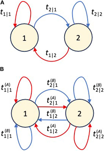
FIGURE 1. (A) Schematic view of a Markov model with two states 1 and 2. Here, t_j|i denotes the probability of the machine to undergo transition from state i to state j. During each transition, an output symbol is created. All red arrows are accompanied by the generation of “A”, while the blue arrows correspond to transitions which generate “B”. In this way, the obtained output symbol is a clear indication of the state of the machine. The state of the machine is, therefore, not hidden. (B) Schematic view of a Markov model with two states 1 and 2. Here, t_j|i denotes the probability of the machine to undergo transition from state i to state j. During each transition, an output symbol is created. All red arrows are accompanied by the generation of “A”, while the blue arrow correspond to transitions which generate “B”. In this way, the obtained output symbol is a clear indication of the state of the machine. The state of the machine is, therefore, not hidden.

If measurement outcomes are ignored or if ensemble averages for a large number of MMs are considered, the states S(n) of individual MMs remain unknown. In this case, we describe the state of the machine by a two-dimensional vector p(n) of the form

Here, p_i(n) is the probability of finding the machine after n time steps in state i and p₁(n) + p₂(n) = 1. Ignoring output symbols, the dynamics of the state vector p(n) can be described by a single transition matrix $T\in \mathcal{T}$ which is defined such that

The operator T contains all the probabilities t_j|i that govern the dynamics of the MM. For example, for the two-state Markov chain in Figure 1A, we have

As is seen in Section 4, the relative simplicity of MMs has the drawback of resulting in only relatively weak correlations in their output sequences.

2.2 Hidden Markov models

Different from MMs, HMMs are stochastic generators whose output symbols do not reveal their state. The internal state remains hidden. Nevertheless, HMMs obey the Markov property as well, and output symbols and transitions depend only on their previous state. Hence, HMMs are characterized by 4-tuples $(\mathcal{S},\mathcal{T},\mathcal{O},\mathit{p}(0))$. Again, $\mathcal{S}$ denotes the relevant state space, and p (0) contains the initial state probabilities. However, $\mathcal{T}$ now contains probabilities for transitioning from a certain state i into a certain state j while creating a certain output symbol. Moreover, $\mathcal{O}$ specifies the possible measurement outcomes, i.e., output symbols. It should be noted that there are two types of HMMs which are called Moore and Mealy [52]. In the first case, the generated stochastic output depends only on the current state of the machine. In the latter case, it depends on the current state and on the observed output symbol, as illustrated in Figure 1B. In this paper, we focus on Mealy HMMs, which contain Moore HMMs as a subset. The reason for looking at these is that we are interested in comparing quantum machines to the most general possible classical stochastic generators.

Here, we are especially interested in machines with only two possible outputs, namely, A and B. In the case of HMMs, this does not restrict the number of internal states. In the following, we denote the hidden states of the HMM by i, with i varying from 1 and N. Suppose $t_{j|i}^{(m)}$ is the probability for a HMM prepared in state i to transition to j while generating output m. In this case, S(n) = i and S (n + 1) = j, as shown in Eq. 1. The probability t_j|i which now equals the sum of the probabilities of generating an A and a B in this case,

Since an external observer has access to the outputs of the machine but not to its hidden states, we now have two transition matrices T_m with m = A, B such that

Using this notation, the state vector p (n + 1) with coordinates p_i (n + 1) which represent the probability of the machine being in state i after n + 1 steps equals

if the state of the machine equaled p(n) after n steps, and output m was obtained in step n + 1. Here, Pr_n(m) denotes the probability of obtaining the output m in step n. Different from MMs, the state vectors p(n) are now real vectors of dimension N.

For example, we can now calculate the probability of an HMM being in a certain state i after n steps when all measurement outputs are ignored. As in the previous subsection, in this case, the dynamics of the state vectors of the HMM can be described by a transition matrix T,

which is the sum of the two sub-transition matrices T_A and T_B. Using this notation,

in analogy to Eq. 1. The matrix element of the total transition matrix T is t_j|i in Eq. 3. If η = (1,1, … ,1)^T is a row vector with all N coordinates equal to 1, then the probability Pr_n+1(m) of getting output m after n + 1 steps equals

We now have all the information needed to simulate all possible individual trajectories of a given HMM with N internal states.

2.3 Hidden quantum Markov models

To obtain quantum versions of HMMs, all we need to do is to replace their hidden states i by quantum states |i⟩. However, being quantum, the allowed internal states of an HQMM are not discrete but continuous. In general, the hidden quantum memory is in a linear superposition of a finite number of discrete quantum states. More concretely, the state |ψ(n)⟩ of an HQMM after n steps can always be written as follows:

where c_i(n) denotes complex coefficients with

As before, the output symbol and the transition of an HQMM depend only on its current internal state, and transitions between subsequent states |ψ(n)⟩ are again specified by linear stochastic process transition matrices [51]. More concretely, given that the output symbol m is measured, the state of the HQMM changes such that

The probability to obtain this outcome for the given initial state |ψ(n)⟩ now equals

which is different from the probability Pr_n+1(m) in Eq. 5. The operator K_m in the above equations is a so-called Kraus operator, which obeys certain constraints [15]. For example, here, we are especially interested in HQMMs with two output symbols, A and B. In this case, probabilities for the two possible measurement outcomes must add up to one. This applies when

where I denotes the identity operator. In this case, the HQMM uses only a single qubit as its internal memory. This means the hidden state of the machine belongs to a two-dimensional state space (N = 2).

Again, if the measurement outputs of the machine are ignored, we cannot know the states |ψ(n)⟩ of individual HQMMs even when their initial state |ψ(0)⟩ is known. In this case, the probability vectors p(n) of HMMs need to be replaced by density matrices ρ(n). These describe the quantum state of the memory averaged over a large ensemble of individual machines and allow us to predict the dynamics of expectation values, like the probability of finding the HQMM at a certain time step in a certain internal state. Instead of Eq. 6, the dynamics of the HQMM is now given by the following equation:

with the superoperator $\mathcal{K}$ defined such that

In other words, the Kraus operators K_A and K_B replace the transition matrices T_A and T_B of HMMs, which we introduced in the previous subsection. For example, the probability Pr_n+1(m) of generating an output m in step n + 1 now equals

where the trace, Tr, denotes the sum of all the diagonal matrix elements.

3 Parametrization, stationary states, and different observable properties

In this section, we parametrize the machines that we introduced in the previous section and highlight the constraints that must be satisfied by each model. In addition, we determine stationary state distributions whenever possible and calculate the probabilities for certain output sequences. For simplicity, we assume, in the following, that all three machines are ergodic due to their finite size and therefore possess a stationary state. The calculated “word probabilities” (probability of a specific output sequence), therefore, apply to the outputs of large ensembles of machines, which all have already reached their stationary states. They also apply to all the words generated by a single machine when averaged over an infinitely long trajectory of output symbols, like the ones illustrated in Figure 2.

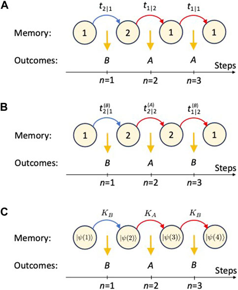
FIGURE 2. Comparison of the mechanisms which lead to the generation of output symbols in the cases of MCs, HMMs, and HQMMs. (A) A Markov chain has two states A and B, and the transition between states over time is governed by the transition probability matrix. The gray arrows show all possible routes of evolving the Markov chain with time, while the red arrow shows a single trajectory. (B) Hidden Markov model evolution over time. Here, the Markov chain has two states A and B, and the transition between states over time is governed by the transition probability matrix. The diagram shows one possible route of evolving the Markov chain with time. (C) Hidden quantum Markov model evolution over time. Here, the hidden quantum Markov model has two states A and B, and the transition between states over time is governed by the transition probability matrix. The diagram shows all possible routes of evolving the hidden quantum Markov model with time.

3.1 Markov Models

From probability theory, we know that the matrix elements of the transition matrix T in Eq. 2 are all between zero and one. In addition, they must obey the condition

for i = 1, 2 to ensure that the machine always transitions into one of its two available states 1 and 2. Since T has four matrix elements and there are two constraints, we can parametrize one-bit MMs using only two independent parameters p and q. More concretely, we write T in the following as

with parameters p, q ∈ [0, 1]. Here, t_1|1 = p, t_2|2 = q, t_2|1 = 1 − p, and t_1|2 = 1 − q. In the next section, we will choose p and q randomly to sample a large set of all possible random machines and study the properties of their output sequences.

The possible output sequences of each machine depend somewhat on their respective initial state p (0). However, if the machine is ergodic and its outputs are ignored for a certain initial minimum amount of time, it soon assumes a stationary state ${\mathit{p}}_{\text{ss}}={(p_1,p_2)}^{\text{T}}$ with

Using Eq. 10 and taking into account that p₁ and p₂ must add up to one, one can show that

These probabilities tell us how likely it is to find a certain machine which is characterized by p and q either in 1 or in 2. Hence, they also equal the probabilities to obtain the outputs A and B at any time n, if the previous outputs of the machine are unknown and cannot be taken into account.

Suppose the machine has initially been prepared in its stationary state p_ss. Then, the probability P (i₁i₂ … i_m) of obtaining the output sequence i₁i₂ … i_m of length m simply equals

with $p_{i_1}$ given in Eq. 12. For example, the probability of creating a word of length m + 2 which starts and ends with the output symbol A and otherwise only contains B’s equals

Alternatively, we could ask, for example, the following question: what is the probability of a word of length m + 2 to start and end with the output symbol A? This probability equals

Probabilities like the above ones are a measure for the complexity of the machine. For example, the probability P_m (A*…*A) can tell us how long correlations persist in the output sequences of a machine. For large m, the probability P_m (A*…*A) tends to p₁ and any knowledge about having been prepared in 1 exactly m + 1 steps earlier is lost.

3.2 Hidden Markov models

As we have seen in Section 2.3, the description of HMMs with two outputs and N internal states requires two transition matrices T_m with N² matrix elements $t_{j|i}^{(m)}$. To identify the number of independent parameters that is needed to numerically simulate all possible HMMs, we first notice that the matrix elements $t_{j|i}^{(m)}$ and t_j|i’s in Eq. 3 are all between zero and one. To, moreover, preserve normality of the probability distribution, we require that

with the matrix element t_j|i defined in Eq. 3. Hence, the transition matrix T in Eq. 4 is an N × N matrix. Given the N constraints in Eq. 16, we, therefore, have N² − N = N(N − 1) free parameters for the matrix T. Once T is fixed, the sub-transition matrix T_A can assume N²-positive free parameters, but these are bounded from above by the matrix elements of T. Once we know T_A, we also know T_B. Hence, in total, the characterization of a Mealy HMM requires N(N − 1) + N² = (2N − 1)N independent parameters.

HMMs are non-deterministic (non-unifilar) since the same transition path can result in different stochastic outputs that increase their complexity [53]. For example, the stationary state is again the distribution vector p_ss which is an eigenvector of the transition matrix T such that Tp_ss = p_ss, as stated in Eq. 11. For HMMs, ${\mathit{p}}_{\text{ss}}={(p_1,p_2,\dots ,p_N)}^{\text{T}}$ is an N-dimensional column vector. In case of ergodicity, the state vector p_ss can be found, for example, numerically by applying T repeatedly to an initial state until the state of the machine remains the same. However, there is no guarantee that an HMM with N internal states has only a single stationary state. For example, an HMM could consist of two independent HMMs with N₁ and N₂ = N − N₁ internal states. In our analysis of HMMs in Section 4, we only consider the stationary state p_ss, which is calculated in a numerical simulation of the machine.

Since the transitions of an HMM are governed by two sub-transitions matrices, namely, T_A and T_B, the probability P (i₁i₂ … i_m) for generating the output sequence i₁i₂ … i_m now reads

More concretely, the probability P_m (AB … BA) in Eq. 14 becomes

If we ignore the m output symbols between the first and the last A, this probability changes into

All three probabilities differ significantly from the probabilities given in Eqs 13–15. As is seen in the next section, HMMs are more likely to produce correlated output sequences than MMs because of their hidden memory.

3.3 Hidden quantum Markov models

Next, let us have a closer observation at how to parametrize HQMMs. Their generalized measurements can be realized by allowing the qubit, which encodes the hidden state of the machine, to interact with an auxiliary quantum system, i.e., an environment, followed by projective measurements on a coarse-grained time scale Δt. In every time step, some hidden information can leak into the environment. Markovianity requires that the ancilla, i.e., the environment, is reset to the same initial state after each measurement. Otherwise, the dynamics of the HQMM would not depend only on the current state of its memory qubit. Figure 2C illustrates the stochastic dynamics of the qubit and the random measurement outcomes that might be produced in a single run of such a machine.

3.3.1 Parametrization of Kraus operators

As in [51, 52], we model HQMMs in the following using the language of open quantum systems and introduce Kraus operators K_A and K_B, which we associate with the output symbols A and B of the machine. To parametrize these Kraus operators, we write them in the following as

The eight complex matrix elements of K_A and K_B can be represented by 16 real parameters. However, as pointed out in Eq. 7, K_A and K_B must obey a matrix equation which implies that

These three equations impose four (real) constraints on the abovementioned 16 real parameters, thereby reducing the total number of free (real) parameters needed to fully characterize HQMMs with one memory qubit to 12. This means a one-qubit HQMM has more free parameters than an HMM with one or two internal states but less free parameters than an HMM with more than two internal states. Nevertheless, as is seen in the following section, it is a more powerful stochastic generator.

3.3.2 Stationary states

If a track record of all measurement outcomes is kept, an HQMM that has initially been prepared in a pure state |ψ(0)⟩ can always be described by a pure state |ψ(n)⟩. However, as mentioned already in the previous section, if this is not the case and measurement outcomes are ignored, the HQMM must be described by a density matrix ρ(n) instead. How this density matrix evolves from one time step to the next is shown in Eq. 8. Its stationary state is, therefore, the density matrix ρ_ss with

with the superoperator $\mathcal{K}$ defined in Eq. 9. Since the HQMM is a two-level system, its stationary state density matrix ρ_ss can be written as follows:

with two real matrix elements, ρ₀₀ and ρ₁₁, and two complex matrix elements, ρ₀₁ and ρ₁₀, and with

In principle, using Eqs 20–24, the stationary state density matrix ρ_ss of HQMMs could be calculated analytically, but the resulting equations do not provide much insight since they still contain 12 free parameters. In the following section, we, therefore, solve the above equations only numerically.

3.3.3 Word probabilities

As before, we now have a closer look at word probabilities. For example, the probability P (i₁i₂ … i_m) in Eqs 13–17 now equals

with the Kraus operators K_m given in Eq. 20. Moreover, the probabilities P_m (AB … BA) and P_m (A*…*A) are now given by the following equations:

which have many similarities with Eqs 18, 19.

4 A comparison of the complexity of MMs, HMMs, and HQMMs

In this final section, we use the parametrization of MMs, HMMs, and HQMMs with two output symbols, which we introduced in the previous section, to study and compare the word probabilities and the time correlations that these machines can produce. As we shall see below, there is not much difference between the complexity of MMs and HMMs. Moreover, we find that increasing the number of internal states of HMMs does not significantly change the correlation range of their output symbols. The possible correlations between output symbols seem to disappear relatively quickly, after only a few time steps. For simplicity, we only consider a subset of all possible HQMMs with only 3 instead of 12 free parameters. Nevertheless, we find that the HQMMs are the most complex of all three machines.

4.1 Simulating HMMs with more than two internal states

First, let us have a closer look at the effect of increasing the number of internal states N of HMMs on their measurement correlations while keeping the number of outcomes equal to two. More concretely, we study the output sequences of HMMs with 2, 3, and 4 internal states. The simulation was carried out as follows: first, we determine a random transition matrix T and random sub-transition matrices T_A and T_B so that the elements of each matrix fulfill the constraints imposed by the model. Then, we determine the corresponding stationary state and evaluate the probabilities P(B) and P(BAAAB). These probabilities are calculated for 10⁵ randomly generated machines and used as the coordinates for the blue dots shown in Figure 3.

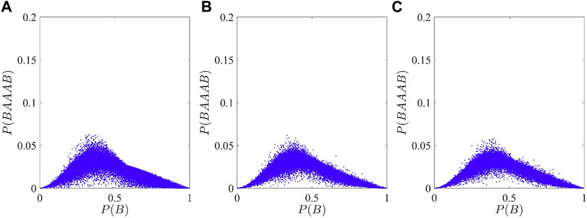
FIGURE 3. Blue dots show the probability P(BAAAB) as a function of P(B) for 10⁵ randomly generated stochastic generators which satisfy the parametrization and conditions imposed on HMMs. The three figures show HMMs with (A) two, (B) three, and (C) four internal states. For each randomly generated machine, we only calculated the probability P(BAAAB) as a function of P(B) of observing the sequence “BAAAB” and “B” once the respective machine reached a stationary state.

As shown in Figure 3, the differences between the three plots are almost negligible. The reason for this might be that we consider machines with only two output symbols. Having only two internal states seems to be sufficient to generate all the correlations that the corresponding HMMs can produce. Expanding the HMMs to include more than two internal states does not improve the performance of the model. If anything, the space that the blue dots occupy in Figures 3B, C seems to be slightly less than the space they occupy in Figure 3A, due to the increasingly large space needed to sample. Increasing the number of internal states seems to make the generation of an “optimal” machine less likely while concentrating the points to a central region. Such sampling problems, while interesting in themselves, do not pose any further interest in the study we consider here. Instead, we satisfy ourselves knowing that the internal state space is not important within the hidden machines (at least with a single output bit). We, therefore, know that increasing hidden resources is not an alternative to generating quantum dynamics, and as such, any increase in complexity is given solely by this new quantum behavior.

4.2 An interesting subset of HQMMs

As is seen in Section 3.3, a complete parametrization of 1-qubit HQMMs requires 12 real parameters. However, to conclude that HQMMs are more complex than HMMs, we only need to identify one stochastic process that can be modeled using an HQMM but cannot be modeled classically. Keeping this in mind, we consider, in the following, HQMMs with Kraus operators K_A and K_B, which can be written as follows:

Here a, φ, and ϑ are real parameters with

It is relatively straightforward to check that the above operators are indeed valid Kraus operators. Instead of 12, we now only have to deal with three free parameters. The stationary states of the above HQMMs can be calculated using Eqs 20 and 21 by proceeding as described in the previous sections.

To show that the above-described generalized measurement is of physical relevance, let us have a closer look at how it could be realized experimentally. As an example, we assume that the memory qubit is a single atom with ground state |1⟩ and an excited state |2⟩. Suppose the initial state of the atom equals

and Γ is the spontaneous decay rate of its excited state. Under the condition of no photon emission, the unnormalized state of the atom equals [17]

after some time Δt since not seeing a photon reveals information about the state of the atom and decreases the probability that the atom is in its excited state. Suppose, we rotate the state of the atom at time Δt by applying the unitary operator

This can be done, for example, using a short strong laser pulse. It is relatively straightforward to check that the overall effect is the implementation of the Kraus operator K_A if the parameter a in Eq. 25 equals exp (−Γ Δt/2). This applies since

in this case. In other words, not seeing a photon in a time interval (0, Δt) followed by the application of U_A is a way of realizing K_A.

However, if the atom emits a photon within the time interval (0, Δt), its unnormalized state equals [17]

at Δt. This state is normalized such that ‖|ψ(Δt)⟩‖² equals the probability of seeing a photon in (0, Δt). Now suppose, the photon emission is followed by the application of the unitary operator

Then, seeing a photon changes the state of the atom, up to a normalization factor into K_B |ψ(0)⟩, since

This means seeing a photon now constitutes a B measurement. One can easily check that the output states and probabilities for measuring the outcomes A and B, respectively, are as one would expect for a generalized measurement with Kraus operators K_A and K_B. In the next subsection, we have a closer look at the output sequences that can be obtained by applying the above-described generalized measurement repeatedly to a memory qubit.

4.3 A comparison of the performance of the machines

This final subsection outlines a comparative analysis of the stochastic properties of the output sequences of the above-introduced MMs, HMMs, and HQMMs with output symbols A and B. In each case, we generate a large number of random machines and determine their stationary-state word probabilities P(BAAAB) and P(B) as previously described, for example, in Section 4.1. For each machine, we then place a single dot in the corresponding figure. The selected sequence for the simulation is “BAAAB” with P(BAAAB) representing the probability of observing the event B subsequent to three consecutive occurrences of AAA, given that the initial outcome is B. In other words, this sequence provides insights into the correlation between two B outcomes separated by multiple observations of A. Figure 4 illustrates that the HQMMs are much more likely to generate word sequences “BAAAB” for a given probability P(B). This means they exhibit a superior performance due to their ability to occupy a larger state space than their classical counterparts, thereby maintaining some information about the history of the machines despite having the Markov property. In summary, despite utilizing only a single qubit as a memory, HQMMs have the capacity to exhibit temporal correlations which cannot be reproduced by linear hidden variable models.

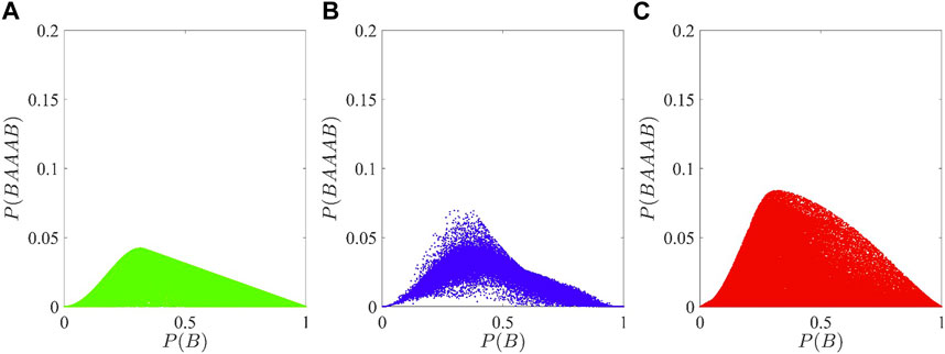
FIGURE 4. Probability P(BAAAB) of observing the sequence “BAAAB” as a function of P(B) for (A) a Markov chain (green), (B) a hidden Markov model with two internal states (blue), and (C) a hidden quantum Markov model (red). Each point corresponds to a randomly generated machine. As one might expect, the comparison of the figures shows in general higher correlations between the measurement outcomes for HQMM than for their classical counterparts, HMMs and MMs, since the red dots cover a much bigger area. For each figure, 10⁵ randomly generated machines were taken into account.

To show that the above behavior is not an outlier but a general feature of HQMMs, we now also have a look at a different word and a different statistical measure. Figure 5 shows a comparison of the performance of MMs, HMMs, and HQMMs with two output symbols with respect to generating the word “BABBAB.” The coordinates of the dots are now given by P(B) and P(BABBAB)/(P(A)²P(B)³). For completely uncorrelated output sequences, this quantity is unity everywhere. Differences from unity, therefore, indicate correlated data. In Figure 5, we clearly see that the difference between the MMs and HMMs is relatively small, although HMMs are more likely to exceed unity than MMs. However, the distribution of the red dots shows that HQMMs are capable of producing relatively strong time correlations that the classical machines are incapable of. This further demonstrates the enhanced complexity of HQMMs and clearly shows that their stochastic dynamics cannot be captured by classical linear hidden variable theories.

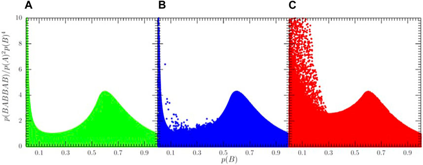
FIGURE 5. Probability P(BABBAB) of observing the sequence “BABBAB” divided by the product of the stationary state probability of each letter of the word, i.e., by P(A)²P(B)³, as a function of P(B) for (A) a Markov chain (green), (B) a hidden Markov model with two internal states (blue), and (C) a hidden quantum Markov model (red). Again, a large number of output trajectories have been created. Similar to Figure 4, we again see an increase in complexity when considering a quantum machine, as demonstrated by the larger area covered in dots. The data here have been generated using the same methodology as Figure 4.

5 Conclusion

This paper compares classical Markov chain-based models, specifically MMs and HMMs with their quantum counterpart, so-called HQMMs. We reviewed the definitions of the three models with a specific emphasis on their parametrization. When increasing the internal states of HMMs with two outputs A and B, we observed that this does not improve the achievable temporal correlations among output sequences. Our simulations show that HMMs with two output symbols do not benefit from having more than two internal states. We then examined the probability of observing two specific output sequences, “BAAAB” and “BABBAB,” for a large number of randomly generated machines. Our simulations of the corresponding word probabilities clearly show that HQMMs can exhibit superior performance. For example, the probabilities P(BAAAB) of certain HQMMs are larger than the maximum probability P(BAAAB) that can be realized with linear classical models. This means quantum physics cannot be captured by classical linear hidden variable theories even in the absence of entanglement. Our work emphasizes the quantumness of temporal correlations in the output sequences produced by generalized measurements and recommends them as an additional resource (which is different from entanglement and usually much easier to produce) for quantum technology applications.

Data availability statement

The raw data supporting the conclusions of this article will be made available by the authors, without undue reservation.

Author contributions

KA: conceptualization, formal analysis, funding acquisition, methodology, software, and writing–original draft. LC: conceptualization, formal analysis, methodology, software, and writing–review and editing. AB: conceptualization, formal analysis, methodology, supervision, and writing–review and editing.

Funding

The author(s) declare financial support was received for the research, authorship, and/or publication of this article. LC acknowledges support from the Foundation for Polish Science within the “Quantum Optical Technologies” project carried out within the International Research Agendas program co-financed by the European Union under the European Regional Development Fund. KA acknowledges the support from the Ministry of Higher Education, Research, and Innovation in the Sultanate of Oman through the National Postgraduate Scholarship Program.

Conflict of interest

The authors declare that the research was conducted in the absence of any commercial or financial relationships that could be construed as a potential conflict of interest.

The author(s) declared that they were an editorial board member of Frontiers, at the time of submission. This had no impact on the peer review process and the final decision.

Publisher’s note

All claims expressed in this article are solely those of the authors and do not necessarily represent those of their affiliated organizations, or those of the publisher, the editors, and the reviewers. Any product that may be evaluated in this article, or claim that may be made by its manufacturer, is not guaranteed or endorsed by the publisher.

References

1. Schrödinger E. Die gegenwärtige situation in der Quantenmechanik. Naturwissenschaften (1935) 23:807–12. doi:10.1063/1.4724105
2. Brukner C, Zukowski M, Zeilinger A. The essence of entanglement, quantum arrangements. Contrib Honor Michael Horne (2021) 117. doi:10.1007/978-3-030-77367-0_6
3. Horodecki R, Horodecki P, Horodecki M, Horodecki K. Quantum entanglement. Rev Mod Phys (2009) 9:865–942. doi:10.1103/revmodphys.81.865
4. Einstein A, Podolsky B, Rosen N. Can quantum-mechanical description of physical reality be considered complete? Phys Rev (1935) 47:777–80. doi:10.1103/physrev.47.777
5. Bell JS. On the Einstein Podolsky rosen paradox. Physics (1964) 1:195–200. doi:10.1103/physicsphysiquefizika.1.195
6. Clauser JF, Horne MA, Shimony A, Holt RA. Proposed experiment to test local hidden-variable theories. Phys Rev Lett (1969) 23:880–4. doi:10.1103/physrevlett.23.880
7. Clauser JF, Shimony A. Bell’s theorem. Experimental tests and implications. Rep Prog Phys (1978) 41:1881–927. doi:10.1088/0034-4885/41/12/002
8. Aspect A, Grangier P, Roger G. Experimental realization of einstein-podolsky-rosen-bohm gedankenexperiment: a new violation of bell’s inequalities. Phys Rev Lett (1982) 49:91–4. doi:10.1103/physrevlett.49.91
9. Kwiat PG, Mattle K, Weinfurter H, Zeilinger A, Sergienko AV, Shih Y. New high-intensity source of polarization-entangled photon pairs. Phys Rev Lett (1995) 75:4337–41. doi:10.1103/physrevlett.75.4337
10. Tittel W, Brendel J, Zbinden H, Gisin N. Violation of Bell inequalities by photons more than 10 km apart. Phys Rev Lett (1998) 81:3563–6. doi:10.1103/physrevlett.81.3563
11. Hensen B, Bernien H, Dréau AE, Reiserer A, Kalb N, Blok MS, et al. Loophole-free Bell inequality violation using electron spins separated by 1.3 kilometres. Nature (2015) 526:682–6. doi:10.1038/nature15759
12. Giustina M, Versteegh MA, Wengerowsky S, Handsteiner J, Hochrainer A, Phelan K, et al. Significant-loophole-free test of bell’s theorem with entangled photons. Phys Rev Lett (2015) 115:250401. doi:10.1103/physrevlett.115.250401
13. Shalm LK, Meyer-Scott E, Christensen BG, Bierhorst P, Wayne MA, Stevens MJ, et al. Strong loophole-free test of local realism. Phys Rev Lett (2015) 115:250402. doi:10.1103/physrevlett.115.250402
14. Aspect A. Closing the door on Einstein and bohr’s quantum debate. Physics (2015) 8:123. doi:10.1103/physics.8.123
15. Kraus K, States, effects, and operations: fundamental notions of quantum theory. Lecture Notes Phys (1983) 190.
16. Bohr N. XXXVII. On the constitution of atoms and molecules. Philos Mag (1913) 26:476–502. doi:10.1080/14786441308634993
17. Hegerfeldt GC. How to reset an atom after a photon detection: applications to photon-counting processes. Phys Rev A (1993) 47:449–55. doi:10.1103/physreva.47.449
18. Dehmelt HG. Proposed 1O ν greater then ν laser fluorescence spectroscopy on T1+mono-ion oscillator II. Bull Am Phys Soc (1975) 20:60.
19. Nagourney W, Sandberg J, Dehmelt H. Shelved optical electron amplifier: observation of quantum jumps. Phys Rev Lett (1986) 56:2797–9. doi:10.1103/physrevlett.56.2797
20. Sauter T, Neuhauser W, Blatt R, Toschek PE. Observation of quantum jumps. Phys Rev Lett (1986) 57:1696–8. doi:10.1103/physrevlett.57.1696
21. Bergquist JC, Hulet RG, Itano WM, Wineland DJ. Observation of quantum jumps in a single atom. Phys Rev Lett (1986) 57:1699–702. doi:10.1103/physrevlett.57.1699
22. Javanainen J. Possibility of quantum jumps in a three-level system. Phys Rev A (1986) 33:2121–3. doi:10.1103/physreva.33.2121
23. Pegg DT, Loudon R, Knight PL. Correlations in light emitted by three-level atoms. Phys Rev A (1986) 33:4085–91. doi:10.1103/physreva.33.4085
24. Cook RJ, Kimble HJ. Possibility of direct observation of quantum jumps. Phys Rev Lett (1985) 54:1023–6. doi:10.1103/physrevlett.54.1023
25. Beige A, Hegerfeldt GC. Quantum zeno effect and light-dark periods for a single atom. J Phys A (1997) 30:1323–34. doi:10.1088/0305-4470/30/4/031
26. Blatt R, Zoller P. Quantum jumps in atomic systems. Eur J Phys (1988) 9:250–6. doi:10.1088/0143-0807/9/4/002
27. Leggett AJ, Garg A. Quantum mechanics versus macroscopic realism: is the flux there when nobody looks? Phys Rev Lett (1985) 54:857–60. doi:10.1103/physrevlett.54.857
28. Paz JP, Mahler G. Proposed test for temporal Bell inequalities. Phys Rev Lett (1993) 71:3235–9. doi:10.1103/physrevlett.71.3235
29. Brukner C, Taylor S, Cheung S, Vedral V. Quantum entanglement in time (2004). arXiv:quant-ph/0402127.
30. Budroni C, Moroder T, Kleinmann M, Gühne O. Bounding temporal quantum correlations. Phys Rev Lett (2013) 111:020403. doi:10.1103/physrevlett.111.020403
31. Zych M, Costa F, Pikovski I, Brukner C. Bell’s theorem for temporal order. Nat Comm (2019) 10:3772. doi:10.1038/s41467-019-11579-x
33. Milz S, Spee C, Xu Z-P, Pollock FA, Modi K, Gühne O. Genuine multipartite entanglement in time. SciPost Phys (2021) 10:141. doi:10.21468/scipostphys.10.6.141
34. Oreshkov O, Costa F, Brukner C. Quantum correlations with no causal order. Nat Commun (2012) 3:1092. doi:10.1038/ncomms2076
35. Goswami K, Romero J. Experiments on quantum causality. AVS Quan Sci (2020) 2:037101. doi:10.1116/5.0010747
36. Debarshi D, Somshubhro B. Quantum communication using a quantum switch of quantum switches. Proc R Soc A (2022) 478:20220231. doi:10.1098/rspa.2022.0231
37. Chiribella G, D’Ariano GM, Perinotti P, Valiron B. Quantum computations without definite causal structure. Phys Rev A (2013) 88:022318. doi:10.1103/physreva.88.022318
38. Araujo M, Costa F, Brukner C. Computational advantage from quantum-controlled ordering of gates. Phys Rev Lett (2014) 113:250402. doi:10.1103/physrevlett.113.250402
39. Ebler D, Salek S, Chiribella G. Enhanced communication with the assistance of indefinite causal order. Phys Rev Lett (2018) 120:120502. doi:10.1103/physrevlett.120.120502
40. Goswami K, Cao Y, Paz-Silva GA, Romero J, White AG. Increasing communication capacity via superposition of order. Phys Rev Res (2020) 2:033292. doi:10.1103/physrevresearch.2.033292
41. Rubino G, Rozema LA, Ebler D, Kristjánsson H, Salek S, Allard Guérin P, et al. Experimental quantum communication enhancement by superposing trajectories. Phys Rev Res (2021) 3:013093. doi:10.1103/physrevresearch.3.013093
42. Garner AJP, Liu Q, Thompson J, Vedral V, Gu M. Provably unbounded memory advantage in stochastic simulation using quantum mechanics. New J Phys (2017) 19:103009. doi:10.1088/1367-2630/aa82df
43. Elliott TJ, Gu M. Superior memory efficiency of quantum devices for the simulation of continuous-time stochastic processes. npj Quan Inf (2018) 4:18. doi:10.1038/s41534-018-0064-4
44. Elliott TJ, Yang C, Binder FC, Garner AJP, Thompson J, Gu M. Extreme dimensionality reduction with quantum modeling. Phys Rev Lett (2020) 125:260501. doi:10.1103/physrevlett.125.260501
45. Blank C, Park DK, Petruccione F. Quantum-enhanced analysis of discrete stochastic processes. npj Quan Inf (2021) 7:126. doi:10.1038/s41534-021-00459-2
46. Milz S, Modi K. Quantum stochastic processes and quantum non-Markovian phenomena. PRX Quan (2021) 2:030201. doi:10.1103/prxquantum.2.030201
47. Korzekwa K, Lostaglio M. Quantum advantage in simulating stochastic processes. Phys Rev X (2021) 11:021019. doi:10.1103/physrevx.11.021019
48. Elliott TJ, Gu M, Garner AJP, Thompson J. Quantum adaptive agents with efficient long-term memories. Phys Rev X (2022) 12:011007. doi:10.1103/physrevx.12.011007
49. Vieira LB, Budroni C. Temporal correlations in the simplest measurement sequences. Quantum (2022) 6:623. doi:10.22331/q-2022-01-18-623
50. Wiesner K, Crutchfield JP. Computation in finitary stochastic and quantum processes. Physica D (2008) 237:1173–95. doi:10.1016/j.physd.2008.01.021
51. Monras A, Beige A, Wiesner K. Hidden quantum Markov models and non-adaptive read-out of many-body states. Appl Math Comp Sci (2011) 3:93. doi:10.48550/arXiv.2310.13815
52. Clark LA, Huang W, Barlow TM, Beige A. Hidden quantum markov models and open quantum systems with instantaneous feedback. In: Interdisciplinary symposium on complex systems. Cham: Springer (2014).
53. Marzen SE, Crutchfield JP. Informational and causal architecture of discrete-time renewal processes. Entropy (2015) 17:4891–917. doi:10.3390/e17074891
54. Cholewa M, Gawron P, Glomb P, Kurzyk D. Quantum hidden Markov models based on transition operation matrices. Quan Inf Process (2017) 16:101. doi:10.1007/s11128-017-1544-8
56. Baum LE, Petrie T. Statistical inference for probabilistic functions of finite state Markov chains. Ann Math Stat (1966) 37:1554–63. doi:10.1214/aoms/1177699147
57. Rabiner LR, Juang BH. An introduction to hidden Markov models. IEEE ASSP Mag (1986) 3:4–16. doi:10.1109/massp.1986.1165342
58. Rabiner LR. A tutorial on hidden Markov models and selected applications in speech recognition. Proc IEEE (1989) 77:257–86. doi:10.1109/5.18626
59. Eddy SR. Hidden markov models. Curr Opin Struct Biol (1996) 6:361–5. doi:10.1016/s0959-440x(96)80056-x
60. P Dymarski, editor. Hidden Markov models, theory and applications. Rijeka, Croatia: IntechOpen Books (2011).
61. Srinivasan S, Gordon G, Boots B. Learning hidden quantum Markov models, international conference on artificial intelligence and statistics. Lanzarote, Spain: PMLR (2017), 09016.
62. Markov V, Rastunkov V, Deshmukh A, Fry D, Stefanski C. Implementation and learning of quantum hidden Markov models (2022), 03796. arXiv:2212.
63. Wood CJ, Biamonte JD, Cory DG. Tensor networks and graphical calculus for open quantum systems. Quan Inf Comput (2015) 15:759–811. doi:10.26421/qic15.9-10-3
64. Binder FC, Thompson J, Gu M. Practical unitary simulator for non-Markovian complex processes. Phys Rev Lett (2018) 120:240502. doi:10.1103/physrevlett.120.240502
65. Clark LA, Stokes A, Beige A. Quantum-enhanced metrology with the single-mode coherent states of an optical cavity inside a quantum feedback loop. Phys Rev A (2016) 94:023840. doi:10.1103/physreva.94.023840
66. Clark LA, Stokes A, Beige A. Quantum jump metrology. Phys Rev A (2019) 99:022102. doi:10.1103/physreva.99.022102
67. Al Rasbi K, Beige A, Clark LA. Quantum jump metrology in a two-cavity network. Phys Rev A (2022) 106:062619. doi:10.1103/physreva.106.062619
Keywords: quantum resources, quantum measurement and entanglement, open quantum systems, hidden Markov model, hidden quantum Markov models
Citation: Al Rasbi K, Clark LA and Beige A (2024) Quantum physics cannot be captured by classical linear hidden variable theories even in the absence of entanglement. Front. Phys. 12:1325239. doi: 10.3389/fphy.2024.1325239
Received: 20 October 2023; Accepted: 29 January 2024;
Published: 29 February 2024.
Edited by:
Craig Martens, University of California, Irvine, United StatesReviewed by:
Marika Taylor, University of Southampton, United KingdomLaszlo Gyongyosi, Budapest University of Technology and Economics, Hungary
Copyright © 2024 Al Rasbi, Clark and Beige. This is an open-access article distributed under the terms of the Creative Commons Attribution License (CC BY). The use, distribution or reproduction in other forums is permitted, provided the original author(s) and the copyright owner(s) are credited and that the original publication in this journal is cited, in accordance with accepted academic practice. No use, distribution or reproduction is permitted which does not comply with these terms.
*Correspondence: Almut Beige, a.beige@leeds.ac.uk