Numerical simulation of hydraulic fracture propagation in fractured reservoir using global cohesive zone method
 Xiaotian Song
 Hongyan Liu*
 - School of Engineering and Technology, China University of Geosciences (Beijing), Beijing, China
Natural fractures in reservoirs have a significant influence on hydraulic fracturing propagation. However, existing analyses have neglected the effect of natural fracture deformation parameters, including crack normal stiffness and shear stiffness on hydraulic fracturing. Therefore, a fractured reservoir model is established using ABAQUS to consider the effect of crack deformation parameters on hydraulic fracturing. A program for inserting global cohesive elements is developed to overcome the limitation of the basic cohesive elements only propagating along the preset path. Further, the bilinear traction-separation constitutive model is used to describe crack initiation and propagation. The analysis focuses on the effect of in situ stress conditions, natural fracture strength parameters (e.g., crack bonding strength), natural fracture deformation parameters (e.g., crack normal and shear stiffness), fracturing-fluid injection rate, and fracturing-fluid viscosity on hydraulic fracturing propagation. The results reveal that the hydraulic fracture initiation pressure increases with the horizontal stress difference, crack bonding strength, injection rate, and fracturing-fluid viscosity but decreases with increasing crack normal and shear stiffness. Additionally, lowering the horizontal stress difference, crack bonding strength, normal and shear stiffness, and fracturing-fluid viscosity results in a more complex fracture network. The total hydraulic fracture length and area increase with the horizontal stress difference and injection rate but decrease with increasing bonding strength, normal and shear stiffness, and fracturing-fluid viscosity. A higher crack bonding strength, crack normal stiffness, shear stiffness, and fracturing-fluid viscosity can improve the hydraulic fracture width and reduce the risk of sand plugging.
1 Introduction
Hydraulic fracturing technology is critical for geothermal and shale gas exploitation and has been widely applied in recent years [1]. Numerous geological investigations and field studies have revealed that natural fractures significantly affect the mechanical properties of reservoirs [2–4]. The natural fractures activate, propagate, and coalesce, forming an effective thermal or gas production channel. Similarly, the natural fracture physical and mechanical (such as length, dip angle, friction coefficient, and deformation parameter) characteristics critically influence hydraulic fracture propagation and, thus, urgently require further study.
Researchers have conducted many experiments to study the complex interaction between hydraulic fractures and natural fractures. For instance, Daneshy [5] conducted experiments on a formation containing natural fractures and found that the natural fracture strength, approaching angle, and principal stress difference significantly affected the interaction between hydraulic fracture and natural fracture. Blanton [6] confirmed that natural fractures were generally activated by hydraulic fracture under the low-stress difference. Researchers proposed several models based on these experimental results for predicting crack interactions. Renshaw and Pollard [7] proposed a criterion for predicting hydraulic fracture behavior after crossing orthogonal cracks, which was verified through comparisons with the experiment results. Gu et al. [8] improved the criterion and predicted nonorthogonal cracks. In addition, researchers considered other factors, such as crack properties [9], fluid viscosity, and injection rate [10], within the frame of the aforementioned criterion. Although they can judge the interaction between natural fracture and hydraulic fracture, these criteria only consider a single crack. However, a complex network is always generated during hydraulic fracturing, and the existing criteria cannot describe crack initiation and propagation induced by hydraulic fracturing in fractured reservoirs.
Numerical simulation can be used to simultaneously investigate the complex propagation of cracks and the influence of a variety of factors. Currently, the finite element method is widely utilized for simulating hydraulic fracture propagation, facilitating an approximation of crack propagation through element failure [11]. In comparison to traditional finite element methods, the extended finite element method [12] accurately simulates actual crack propagation. It can intuitively represent crack propagation, but the interaction between multiple cracks requires further improvement. The discrete element method can directly simulate crack interactions [13], but it is not suitable for actual engineering practice because the calculation scale is small [14]. The finite discrete element method [15], which couples the finite element method and discrete element method, has also been successfully applied to hydraulic fracturing [16], but the fluid leak-off is ignored in the simulation of hydraulic fracture propagation.
The cohesive zone model (CZM) can overcome the above limitations. It utilizes the traction separation law to determine material damage and failure. Barenblatt [17] first utilized this method to simulate crack propagation in brittle materials. Later, Guo et al. [18] proposed a CZM for studying hydraulic fractures in layered reservoirs, considering the effects of geological and fracturing-fluid parameters. Wang [19] studied multistage fracturing and interference between cracks using XFEM and CZM. Manchanda et al. [20] proposed a three-dimensional CZM considering rock heterogeneity and multicluster hydraulic fracture propagation. Baykin et al. [21] proposed an inhomogeneous poroelastic medium hydraulic fracturing cohesive model for studying the effect of permeability on the hydraulic fracture process. Yu et al. [22] proposed an adaptive insertion method for three-dimensional cohesive elements to study the effect of pumping plans, such as pumping hesitations, on the development of naturally fractured reservoirs. However, the original CZM could only simulate the crack propagation process along a preset path. Afterward, the propagation path of a large-scale complex fracture network was successfully simulated [23–28] by inserting zero-thickness cohesive elements around the solid element. Researchers have utilized the global cohesive zone model to conduct a series of studies on geological and operation parameters for hydraulic fracturing, such as in situ stress conditions, fluid injection rate, fluid viscosity, natural fractures geometry parameter, and strength parameter [29–31]. Natural fracture physical and mechanical properties can be described by the three types of parameters, namely, geometry (e.g., crack length and dip angle), strength (e.g., crack friction coefficient or bonding strength), and deformation parameters (e.g., crack normal and shear stiffness). Notably, researchers [32, 33] have found that the natural fracture deformation parameters affect the mechanical properties of a rock mass, including its strength and wing-crack initiation angle. However, these studies ignored the effect of natural fracture deformation parameters when considering hydraulic fracturing in fractured reservoirs.
Therefore, the effects of the natural fracture deformation parameter on hydraulic fracturing should be considered. A fractured reservoir mode based on statistical crack results is established to fully study the effect of natural fracture properties on hydraulic fracturing. The traditional CZM only allows the crack to propagate along preset paths. Therefore, a Python program for inserting global cohesive pore pressure elements is developed to ensure the hydraulic fracture can propagate along any direction, thereby simulating the evolution of a complex fracture network. Furthermore, crack initiation was described using the bilinear traction-separation constitutive model. Accordingly, the entire process of hydraulic fracturing in a cracked reservoir was simulated. This study focuses on the effect of in situ stress conditions, natural fracture strength parameters (crack bonding strength), deformation parameters (crack normal and shear stiffness), fracturing-fluid injection rate, and fracturing-fluid viscosity on hydraulic fracturing.
2 Overview of the numerical calculation model
2.1 Constitutive model and damage criterion of cohesive element
Researchers proposed a CZM for the fracture analysis of metal materials [17, 34]. This method avoids the problem of stress singularity at the crack tip in linear elastic fracture mechanics. Hillerborg [35] then extended it to quasi-brittle materials, making CZM applicable to rock fracture analysis.
In this study, the cohesive element is used to simulate hydraulic and natural fractures in the reservoir model. The bilinear-traction separation constitutive model describes the relationship between traction force and displacement [36], as shown in Figure 1. The bilinear-traction separation constitutive model comprises two stages: a) the elastic deformation stage with constant stiffness and b) the damage evolution stage with decreasing stiffness. Stress and displacement have a linear relationship during the elastic deformation stage. Further, the element enters the damage evolution stage at δ0m.
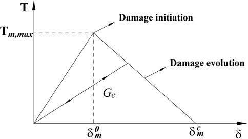
FIGURE 1. Bilinear traction-separation constitutive model.
In this study, the quadratic nominal stress law criterion is applied to identify damage initiation:
where tn is normal stress, tt and ts denote the first, and the second shear stress; tn,max, tt,max and ts,max refer to the tensile, the first, and the second shear strength, respectively; < > is the Macaulay bracket.
Once the damage critical point is reached, the rock will exhibit softening characteristics. The damage variable D describes the rock damage degree, which is defined by δ, δ0m and δcm:
When D = 1, the cohesive element completely fails. The element stiffness matrix K’ is determined by the initial stiffness K and the damage variable D:
2.2 Fluid–solid coupling equation of rock
The total stress inside a reservoir comprises effective stress and pore pressure because of the porous property of the material. The equilibrium equation can be formulated as follows based on the principle of virtual work [37]:
where σ‾ is the effective stress; the δε and δv are the matrix of virtual strain and virtual velocity, respectively; pw is pore pressure; I is the unit matrix; t and f are the surface traction vector and body force vector, respectively.
2.3 Continuity equation of fluid flow in porous medium
The mass conservation equation is used to describe the continuity of fluid flow in porous media [38]:
where vwi is seepage velocity in porous media and ϕ is the porosity of the formation.
In this study, the fracturing fluid was assumed to be an incompressible Newton fluid, with the fluid flow conforming to Darcy’s law in the porous formation. The relationship between seepage velocity and pore pressure gradient is given by (38):
where k is the matrix of permeability of porous media and gi is the gravity acceleration vector.
2.4 Fluid flow within crack
The fluid flow within the cohesive element comprises normal flows (seepage normal to the element surface) and tangential flows (flow along the direction of element length), as shown in Figure 2. The governing equation of fluid flow within the crack can be describe as follows:
where q is the tangential flow rate within the crack; d is the gap opening; qt and qb denote fluid rates into top and bottom surfaces, respectively; Q(t) and δ(x,y) are the injection rate and Dirac delta function, respectively.
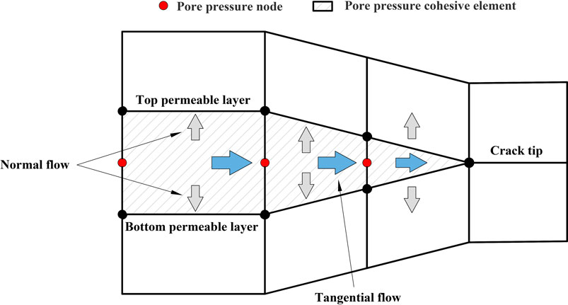
FIGURE 2. Fluid flow in cohesive elements.
For the Newtonian fluids with viscosity μ, the tangential flow inside the crack is approximated as parallel plate flow, and the local flow rate q can be determined from the pressure gradient and local crack width [39]. The tangential flow is calculated as follows:
where ∇p is the pressure gradient along the cohesive element; μ is the fluid viscosity.
Normal flow and fracturing-fluid leak-off are usually simplified using the leakage coefficient:
where ct and cb denote the fluid leak-off coefficients at the top and bottom permeable layer, respectively; pi denotes the midface pressure; and pt and pb denote the pore pressures on the top and bottom permeable layer, respectively.
2.5 Global cohesive zone method
Unlike the basic CZM model in Abaqus, which can only simulate crack propagation along the preset path, the global cohesive zone method can insert cohesive elements along the edge between every two neighboring elements during preprocessing, thus predicting the path and propagation direction of the hydraulic fracture.
As an example, the model in Figure 3 illustrates the process of inserting global cohesive elements with Python script:
(1) Reading the input file and recording the occurrence number of every node in the model as xi. The model in Figure 3 consists of four elements, where node 2 appears in Elem1 and Elem2. Therefore, the occurrence number of node 2 is 2, that is, x2 = 2. Moreover, node 5 appears in elem1, Elem2, Elem3, and Elem4, so the occurrence number of node 5 is 4, that is, x5 = 4.
(2) Creating new nodes at the original coordinate based on the occurrence number of each node. x-1 new nodes are created at the original coordinates based on the occurrence number xi. The new node creation process is shown in Figure 3. For node 2, a common node of Elem1 and Elem2, the occurrence number of node 2 is 2, and a new node 12 should be generated. The node occurrence number for node 5 is 4, as it is a common node of four elements. Therefore, three new nodes need to be generated and named, that is 15, 25, and 35.
(3) Inserting pore pressure cohesive elements. Two critical problems must be addressed when inserting the cohesive pore pressure element. First, the adjacent pore pressure cohesive elements should utilize the same pore pressure node to ensure continuous fluid flow. For instance, node 45 is the shared pore pressure node of four pore pressure elements in Figure 4. Second, the vector cross product is used to ensure the direction of elements and node sequences are correct when inserting the pore pressure cohesive element. For example, the node numbering sequence should start with one edge and end with the other while inserting a cohesive element between Elem1 and Elem4. Further, the pore pressure node direction should be consistent with the starting edge. The correct sequence should be 4, 5, 35, 14, 24, 45, or 35, 14, 4, 5, 45, 24, as shown in Figure 5.
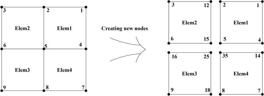
FIGURE 3. New node creation process.
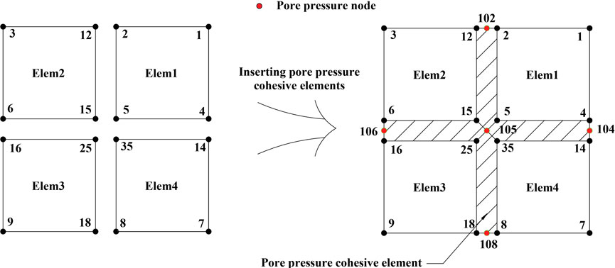
FIGURE 4. Inserting process of pore pressure cohesive element.
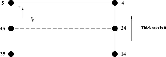
FIGURE 5. Node information of pore pressure cohesive element.
2.6 Model validation
The interference model for hydraulic and natural fractures was established using ABAQUS code to verify the cohesive elements global inserting method, as shown in Figure 6. The model size was 50 m × 50 m. The maximum and minimum horizontal principal stress directions were X and Y, respectively. The 0.5 m CPE4RP element was used to simulate the rock mass, and the COH2D4P element was used to simulate cracks. The quadratic normal stress law criterion was utilized to calculate the crack initiation. A 5 m long crack was set 5 m from the liquid injection point in this model, and α is the approach angle between the hydraulic and natural fracture. The input data in Table 1 were obtained from the cracked specimen of Zhang [40].
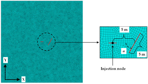
FIGURE 6. Interaction model between hydraulic and natural fractures.
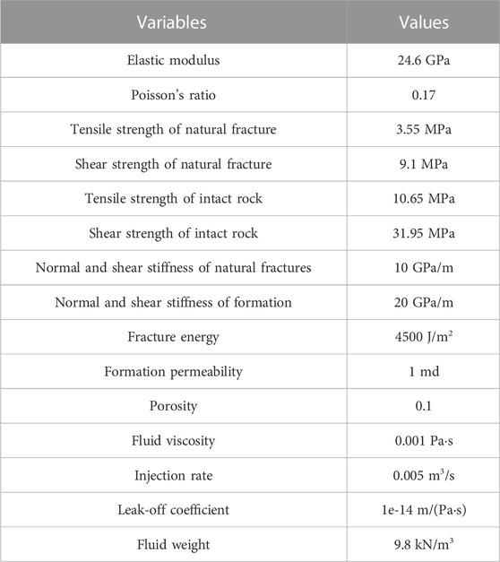
TABLE 1. Model parameters.
The boundary conditions of the calculation model are as follows: an X-direction displacement constraint was applied to the left and right boundaries, whereas a Y-direction displacement constraint was applied to the top and bottom boundaries. In addition, the pore pressure on the model boundary was 0 MPa. To improve the convergence of the numerical simulation, the injection rate was set to increase linearly over time within 30 s.
Next, the interactions between hydraulic and natural fractures for approach angles of 30°, 45°, and 60° were studied. The numerical results for 45° and 60° approach angles are shown in Figure 7. The crack approach angle and horizontal stress ratio were the change parameters. The horizontal stress ratio is the maximum horizontal principal stress ratio to the minimum horizontal principal stress. Compared with the laboratory experiment of Blanton [6], the simulation results demonstrated that when the horizontal stress ratio was 1.2 and the approach angle was 60°, the natural fracture internal pressure was greater than the external pressure and the hydraulic fracture activated and turned along the natural fracture (Figure 7A). Increasing the horizontal stress ratio to 4 resulted in the hydraulic fracture directly crossing the natural fracture, as shown in Figure 7B. When the approach angle decreased to 45° and the horizontal stress ratio was 4, the hydraulic fracture could not activate the natural fracture and was arrested at the natural fracture (Figure 7C). Therefore, the simulation results well-matched the laboratory experiment, which validates the global cohesive elements method.
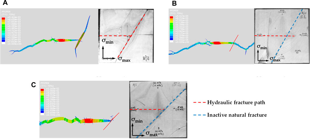
FIGURE 7. Numerical simulation (left) and Blanton experimental results (right). (A) Horizontal stress ratio of 1.2 and approach angle of 60 °; (B) Horizontal stress ratio of 4 and approach angle of 60 °; (C) Horizontal stress ratio of 4 and approach angle of 45 °.
3 Numerical simulation of hydraulic fracture propagation in strata with random cracks
3.1 Numerical model establishment
This study established a reservoir model with random cracks, as shown in Figure 8. The geometric parameters of two crack sets were obtained from the statistical results (Table 2) on the rock mass of the Lancang River dam foundation [41], and the crack center was assumed to be uniformly distributed. The minimum and maximum horizontal principal stress directions were X and Y, respectively. The center point was the liquid injection point, and the perforation direction was consistent with the maximum horizontal principal stress direction. The model size, parameters, element size, and boundary conditions were consistent with the model previously verified in Section 2.6.
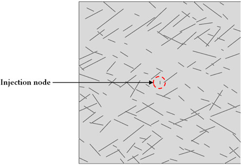
FIGURE 8. Reservoir model with random cracks.
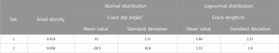
TABLE 2. Geometric parameters of natural fractures.
3.2 Simulation results and analysis
The hydraulic fracture propagation path in a fractured reservoir is quite complex. Moreover, the fracture network formation is affected by various factors, including in situ stress condition, crack bonding strength, crack normal stiffness, crack shear stiffness, fluid injection rate, and fracturing-fluid viscosity. Therefore, we designed six sets of models using different parameters for the numerical calculation (Table 3) and monitored the hydraulic fracture propagation path, injection point pressure, hydraulic fracture total area, and total length. The horizontal stress difference in Table 3 represents the difference between the maximum and minimum horizontal principal stress. The strength degradation ratio in Table 3 represents the intact rock strength ratio to crack bonding strength. The injection point pressure represents the pore pressure at the fracturing-fluid injection point, the total hydraulic fracture area is the area sum of activated cohesive elements, and the total hydraulic fracture length is the total length of activated cohesive elements.
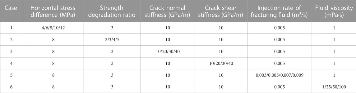
TABLE 3. Numerical calculation schemes.
3.2.1 Effect of horizontal stress difference (HSD) on hydraulic fracture propagation
The numerical simulation results of maintaining the minimum horizontal stress at 10 MPa while the horizontal stress difference increases to 4, 6, 8, 10, and 12 MPa are shown in Figures 9, 10.
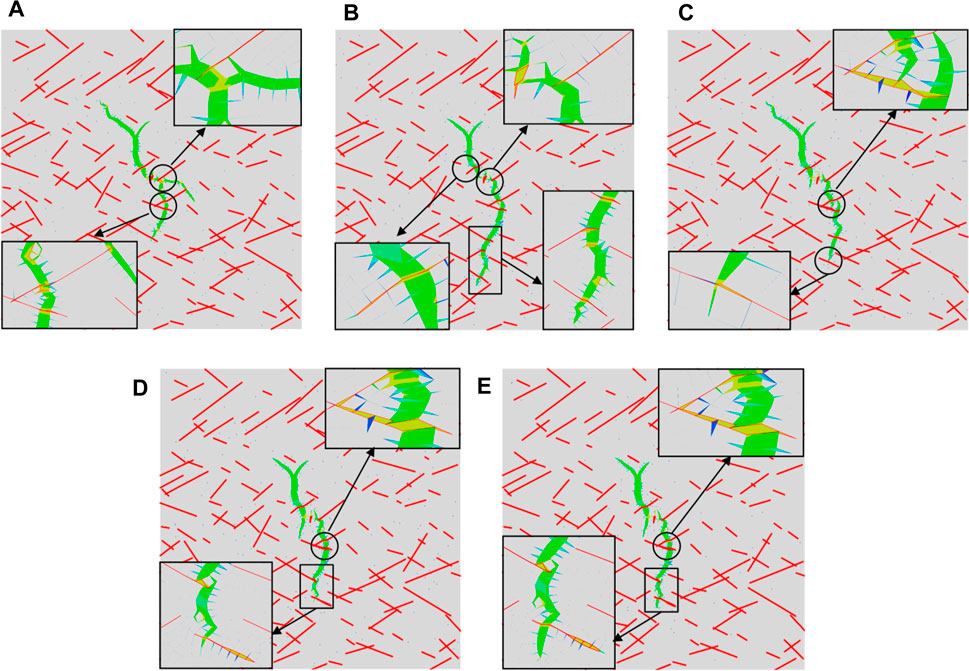
FIGURE 9. Hydraulic fracture propagation path under different HSD. (A) HSD = 4 MPa; (B) HSD = 6 MPa; (C) HSD = 8 MPa; (D) HSD = 10 MPa; (E) HSD = 12 MPa.
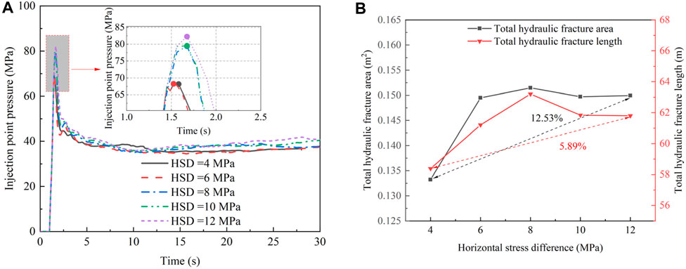
FIGURE 10. (A) Injection point pressure–time history curve for different HSD; (B) Effect of HSD on total hydraulic fracture area and length.
When the horizontal stress difference was 4 MPa, the maximum horizontal stress and natural fractures controlled the main direction of hydraulic fracture propagation. However, the hydraulic fracture exhibits multiple turning and branching behaviors along the trend direction of the crack group. This resulted in a complex fracture network and produced multiple secondary cracks. As the horizontal stress difference increased to 6 and 8 MPa, the effect of natural fractures on the propagation was weakened, and the propagation direction tended toward the maximum horizontal stress direction. The crack branches were restrained, and the hydraulic fracture shape tended to be single. Meanwhile, the hydraulic fracture activated and crossed several natural fractures during propagation. Nevertheless, the horizontal stress difference and crack groups jointly affected the opening resistance of the natural fractures, which prevented the hydraulic fracture from fully activating the natural fractures. When the stress difference reached 10 MPa or 12 MPa, the propagation direction of the main crack was almost parallel to the direction of the maximum horizontal stress. Further, the hydraulic fracture propagation length increased significantly, and multiple natural fractures were activated.
The crack initiation pressure increases with increasing horizontal stress difference, as shown in Figure 10A. Due to the high horizontal stress difference, natural fractures require high amounts of energy to be activated, which increases their resistance to hydraulic fracture propagation. As shown in Figure 10B, when the stress difference exceeded 10 MPa, the total hydraulic fracture area and length no longer increased with the horizontal stress difference but slightly decreased. The high horizontal stress difference results in hydraulic fracture tending to cross the natural fractures directly. Moreover, the main crack exhibits clear propagation guidance, and the growth of the crack branch reduces. Therefore, a certain stress difference is conducive to opening more natural fractures and forming a complex fracture network. However, an excessive stress difference will limit reservoir development.
3.2.2 Effect of crack bonding strength on hydraulic fracture propagation
Generally, natural fracture strength is weaker than the intact rock mass strength. The ratio of intact rock strength to natural fracture strength is termed the strength degradation ratio (SDR) and is used to study the effect of crack bonding strength on hydraulic fracture propagation. A larger SDR represents a lower bonding strength of natural fractures and failure susceptibility. The numerical simulation results for SDR values of 5, 4, 3, and 2 are shown in Figures 11, 12.
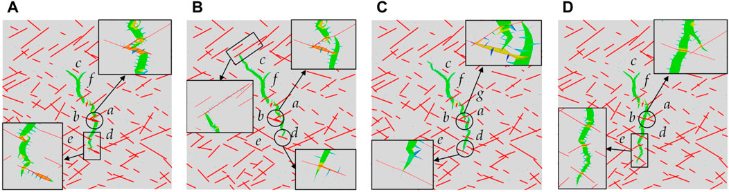
FIGURE 11. Hydraulic fracture propagation path under different crack bonding strengths. (A) SDR = 5; (B) SDR = 4; (C) SDR = 3; (D) SDR = 2.
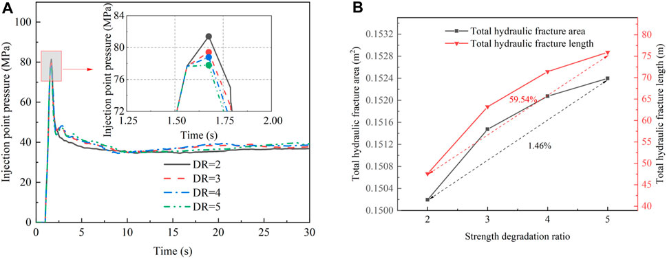
FIGURE 12. (A) Injection point pressure–time history curve for different crack bonding strength; (B) Effect of crack bonding strength on total hydraulic fracture area and length.
When the SDR was 5, the hydraulic fracture tended to activate more natural fractures. The hydraulic fracture sequentially activated cracks a and b, propagated along crack b, and turned toward the direction of the maximum horizontal principal stress. Multiple natural fractures were activated at the far end. When SDR decreased to 4, the hydraulic fracture activated cracks a and b sequentially, terminating with fracture d. Moreover, hydraulic fracture branches were generated near crack c due to the effect of natural fractures. At a SDR of 3, the number of natural fractures activated by hydraulic fracture significantly decreased as the crack bonding strength increased. When SDR decreased to 2, the hydraulic fracture directly crossed several cracks and propagated along the direction of the maximum horizontal principal stress. Notably, the complexity of the hydraulic fracture significantly decreased.
Figure 12A shows that the crack initiation pressure decreased with increasing SDR. The lower crack bonding strength predisposes the reservoir to damage. The total hydraulic fracture area and length increase with decreasing crack bonding strength, as shown in Figure 12B. Many natural fractures were activated during the propagation of the hydraulic fracture, which improved the total hydraulic fracture area and length. Therefore, the lower crack bonding strength promotes a complex hydraulic fracture network. However, the change in the total length is much greater than the total area, indicating that a high crack bonding strength improves the hydraulic fracture width and lowers the risk of sand plugging.
3.2.3 Effect of crack normal stiffness on hydraulic fracture propagation
The numerical simulation results when the crack normal stiffness increases from 10 GPa/m to 20 GPa/m, 30 GPa/m, and 40 GPa/m are shown in Figures 13, 14.
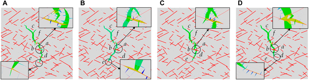
FIGURE 13. Hydraulic fracture propagation path under different crack normal stiffnesses. (A) kn = 10 GPa/m; (B) kn = 20 GPa/m; (C) kn = 30 GPa/m; (D) kn = 40 GPa/m.
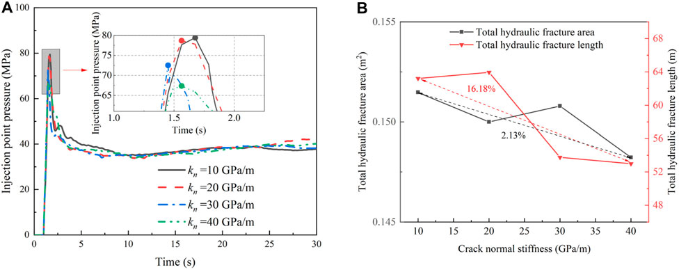
FIGURE 14. (A) Injection point pressure–time history curve for different crack normal stiffnesses; (B) Effect of crack normal stiffnesses on total hydraulic fracture area and length.
When the crack normal stiffness was 10 GPa/m, the hydraulic fracture crossed crack a and activated crack b, then turned along crack b and continued to propagate along the direction of the maximum horizontal principal stress. The hydraulic fracture deflected and branched when approaching crack c due to the interaction of in situ stress and natural fractures. When the crack normal stiffness increased to 20 GPa/m and 30 GPa/m, the hydraulic fracture produced multiple branches around the intersection of cracks a and b, which was caused by the stress concentration generated near the cross cracks. The hydraulic fracture then activated and crossed crack b and continued to propagate. When the normal stiffness reached 40 GPa/m, the dominant direction of the hydraulic fracture was still controlled by the maximum principal stress. The hydraulic fracture activated crack a and b successively, but the crack branches generated at cross cracks a and b are restrained. Finally, the hydraulic fracture was arrested at crack d.
Figure 14A shows that the crack initiation pressure decreases with increasing crack normal stiffness. When the normal stiffness was 20 GPa/m, the total hydraulic fracture length slightly increased due to the additional crack branches at intersection cracks a and b. Subsequently, the total hydraulic fracture length decreased with increasing crack normal stiffness, and the total area simultaneously decreased. These indicate that increasing the crack normal stiffness limits the total hydraulic fracture length and area, which reduces the complexity of the hydraulic fracture network. However, the change degree in total length was much greater than the total area, which indicated that higher crack normal stiffness improves the hydraulic fracture width and reduced the risk of sand plugging.
3.2.4 Effect of crack shear stiffness on hydraulic fracture propagation
The numerical simulation results when the crack shear stiffness increased from 10 GPa/m to 20 GPa/m, 30 GPa/m, and 40 GPa/m are shown in Figures 15, 16.
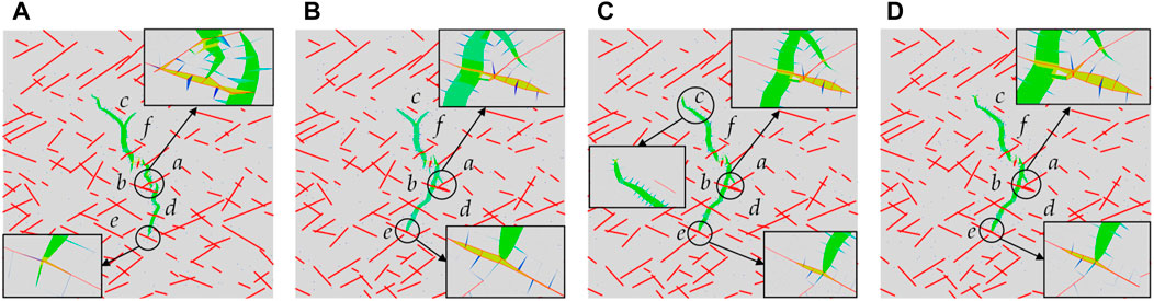
FIGURE 15. Hydraulic fracture propagation path under different crack shear stiffnesses. (A) ks = 10 GPa/m; (B) ks = 20 GPa/m; (C) ks = 10 GPa/m; (D) ks = 10 GPa/m.
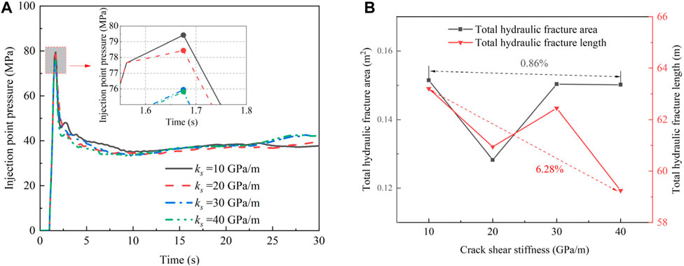
FIGURE 16. (A) Injection point pressure–time history curve for different crack shear stiffness; (B) Effect of crack shear stiffness on total hydraulic fracture area and length.
As the crack shear stiffness increased from 10 GPa/m to 20 GPa/m, the hydraulic fracture changed from directly crossing crack a and opening crack b to activating and directly crossing crack b. Meanwhile, small branches were generated around the intersection of cracks a and b. Afterward, the main crack continued to propagate along the maximum horizontal stress direction. Hydraulic fracture branches occurred when approaching crack c, and another direction arrest occurs at crack e. When the crack shear stiffness increased to 30 GPa/m or 40 GPa/m, the small branches produced by hydraulic fracture decreased considerably. The hydraulic fracture stopped producing branches, turning instead when approaching crack c, which indicated that the increase in crack shear stiffness limited the generation of hydraulic crack branches and increased the integrity of the stratum.
Figure 16A shows that the crack initiation pressure decreased with increasing crack normal stiffness. when the shear stiffness was 20 GPa/m, the total hydraulic fracture area significantly decreased due to the length reduction of crack branches near crack c. Subsequently, the total hydraulic fracture area slightly decreased with increasing the crack shear stiffness. The total hydraulic fracture length exhibited a fluctuating downward trend with an increase in the crack shear stiffness, which indicated that the total hydraulic fracture length significantly decreased with increasing crack shear stiffness. Meanwhile, the hydraulic fracture width continuously increased due to the slight change in the total hydraulic fracture area, and reduced the risk of sand plugging.
3.2.5 Effect of fracturing-fluid injection rate on hydraulic fracture propagation
The numerical simulation results when the fracturing-fluid injection rate increase from 0.003 m3/s to 0.005 m3/s, 0.007 m3/s, and 0.009 m3/s are shown in Figures 17, 18.
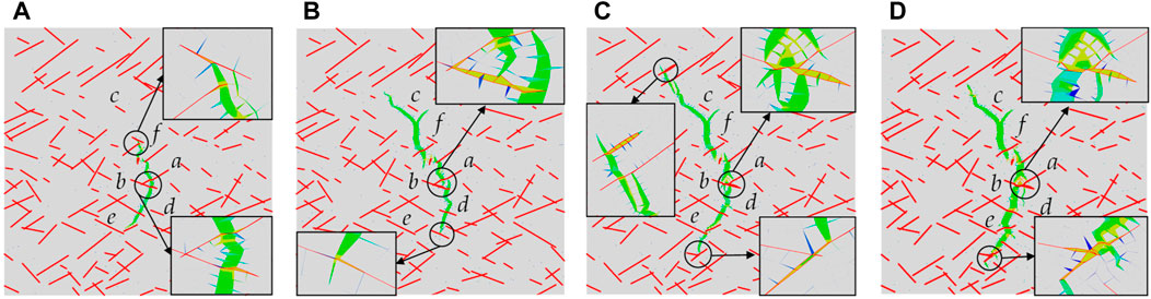
FIGURE 17. Hydraulic fracture propagation path under different fracturing-fluid injection rates. (A) Q = 0.003 m3/s; (B) Q = 0.005 m3/s; (C) Q = 0.007 m3/s; (D) Q = 0.009 m3/s.
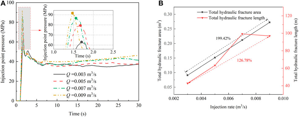
FIGURE 18. (A) Injection point pressure–time history curve for different fracturing-fluid injection rates; (B) Effect of injection rate on total hydraulic fracture area and length.
When the liquid injection rate was 0.003 m3/s, the hydraulic fracture propagated along the maximum principal stress direction and was arrested at crack f. The hydraulic fracture at the other end propagated and crossed multiple cracks, and the main crack produced no marked branches. When the liquid injection rate increased to 0.005 m3/s, the stress in the crack tip increased, and many small branches were generated. Therefore, the total length of the hydraulic fracture increased considerably. When the liquid injection rate reached 0.007 m3/s and 0.009 m3/s, the hydraulic fracture produced many branches at the intersection of cracks a and b, activating several natural fractures at the far end. The complexity of the fracture network also increased significantly. Meanwhile, hydraulic fracture tended to activate more natural fractures, and the main crack still propagated parallel to the maximum principal stress direction.
Figure 18A shows that fluid injection pressure increased with increasing fluid injection rate. A higher injection pressure activated more cracks in the reservoir and formed a more complex hydraulic fracture network [42]. The total hydraulic fracture area and length increased with the fluid injection rate, as shown in Figure 18B. Therefore, increasing the fluid injection rate can effectively improve the degree of reservoir fracturing.
3.2.6 Effect of fracturing-fluid viscosity on hydraulic fracture propagation
The numerical simulation results when the fracturing-fluid viscosity increases from 1 mPa·s to 25 mPa·s, 50 mPa·s, and 100 mPa·s are shown in Figures 19, 20.
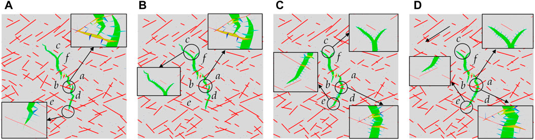
FIGURE 19. Hydraulic fracture propagation path under different fracturing-fluid viscosities. (A) μ = 1 mPa·s; (B) μ = 1 mPa·s; (C) μ = 1 mPa·s; (D) μ = 1 mPa·s.
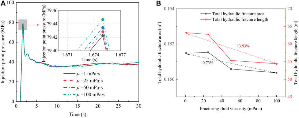
FIGURE 20. (A) Injection point pressure–time history curve for different fracturing-fluid viscosities; (B) Effect of fracturing-fluid viscosity on total hydraulic fracture area and length.
When the fracturing-fluid viscosities were low—for instance, 1 mPa·s and 25 mPa·s—the hydraulic fracture crossed crack a and activated crack b, propagating along the latter. Afterward, the hydraulic fracture continued to propagate along the direction of the maximum principal stress. The hydraulic fracture deflected and developed branches near crack c, forming a complex fracture network. Although the hydraulic fracture had branches near crack c, the crack propagation length of the branches was shorter than that when the viscosity of fracturing-fluid was 1 mPa·s or 25 mPa·s as the fracturing-fluid viscosity increased to 50 or 100 mPa·s. Meanwhile, at cross cracks a and b, hydraulic fracture tended to cross, rather than open, crack b directly. Therefore, the complexity of the hydraulic fracture was considerably restrained.
Figure 20A shows that crack initiation pressure slightly increased with increasing fracturing-fluid viscosity. Figure 20B shows that the total hydraulic fracture area and length decreased significantly with increasing fracturing-fluid viscosity, indicating that higher fracturing-fluid viscosity limits the development of hydraulic fracture. However, the change degree in total length is much greater than the total area, indicating that higher fracturing-fluid viscosity improves the hydraulic fracture width and reduces the risk of sand plugging. Therefore, different fracturing-fluid viscosities can be employed for different construction stages to obtain the best fracturing effect [43].
4 Conclusion and discussions
This study establishes a fractured reservoir model based on statistical crack results. It considers the effect of natural fracture deformation parameters in the hydraulic fracturing analysis, which was ignored in previous studies. The cohesive element with the bilinear traction-separation constitutive model is used to simulate potential cracks. Meanwhile, Python is used to develop the program for inserting global cohesive elements. This method overcomes the limitation of the original insertion method in Abaqus, which can only simulate presetting crack propagation path.
In addition, the effects of in situ stress conditions, natural fracture strength parameters (crack bonding strength), deformation parameters (crack normal stiffness and shear stiffness), fracturing-fluid injection rate, and fracturing-fluid viscosity on hydraulic fracturing propagation are studied. The following conclusions are drawn from this numerical study:
1) The crack initiation pressure increases with increasing horizontal stress difference. When the horizontal stress difference is low, maximum horizontal stress and natural fractures affect the propagation direction of hydraulic fracture. When the horizontal stress difference is large, the direction of hydraulic crack propagation is dominated by the maximum horizontal principal stress. A low horizontal stress difference promotes complex fracture networks, but the total hydraulic fracture length and area are small relative to the high ground stress differences; however, an excessively large horizontal stress difference limits the generation of hydraulic fracture branches and the establishment of complex hydraulic fracture networks.
2) With increasing crack bonding strength, the crack initiation pressure continuously increases. Further, hydraulic fractures tend to cross natural fractures rather than activate them. Meanwhile, the total hydraulic fracture length and area decrease with increasing crack bonding strength, which limits the development of fracture reservoirs. However, a higher crack bonding strength improves the hydraulic fracture width and lowers the risk of sand plugging.
3) Decreasing the crack normal and shear stiffness increases the crack initiation pressure to varying degrees. More significant normal and shear stiffness limits the total hydraulic fracture length and area, which is unfavorable for reservoir development. In addition, the effect of normal stiffness is more significant that of shear stiffness. Therefore, to fully exploit the geological conditions of the reservoir, the in situ stress, distributions, and parameters of natural fractures should be accurately measured before drilling to guide the construction scheme design.
4) Increasing the fracturing-fluid injection rate can significantly increase the total hydraulic fracture length and area. Furthermore, a higher pore pressure at the injection point promotes the hydraulic fracture initiation and propagation. Lowering fracturing-fluid viscosity tends to activate multiple natural fractures, which is beneficial for forming complex fractures; further, a higher fracturing-fluid viscosity improves the hydraulic fracture maximum width and reduces the risk of sand plugging. Therefore, the fracturing-fluid with different viscosities can be used for different fracturing operations to improve the fracturing effect.
5) This paper only considered the straight crack in simulation. However, the crack shape in engineering rock masses is irregular, and the effect of crack roughness needs to be further considered for the fractal dimension [44]. In addition, only the single-phase flow problem is considered in this paper. However, two-phase flow problems widely exist in oil and gas reservoirs, including gas–water and oil-water two-phase flows. They can be studied under the fractal approach [45, 46]. These aspects will be considered in further work.
Data availability statement
The original contributions presented in the study are included in the article/supplementary material, further inquiries can be directed to the corresponding author.
Author contributions
XS: Conceptualization, Data curation, Investigation, Methodology, Software, Writing–original draft. HL: Conceptualization, Data curation, Funding acquisition, Project administration, Resources, Supervision, Writing–review and editing. XZ: Funding acquisition, Project administration, Resources, Software, Supervision, Writing–review and editing.
Funding
This work was supported in part by Project (2022XAGG0500) supported by Xiong’an New Area Science and Technology Innovation Special Project of the Ministry of Science and Technology; Project (8222031) supported by the Natural Science Foundation of Beijing; Project (42172342) supported by the National Natural Science Foundation of China.
Conflict of interest
The authors declare that the research was conducted in the absence of any commercial or financial relationships that could be construed as a potential conflict of interest.
Publisher’s note
All claims expressed in this article are solely those of the authors and do not necessarily represent those of their affiliated organizations, or those of the publisher, the editors and the reviewers. Any product that may be evaluated in this article, or claim that may be made by its manufacturer, is not guaranteed or endorsed by the publisher.
References
1. Weng X. Modeling of complex hydraulic fractures in naturally fractured formation. J Unconventional Oil Gas Resour (2015) 9:114–35. doi:10.1016/j.juogr.2014.07.001
2. Raterman KT, Farrell HE, Mora OS, Janssen AL, Gomez GA, Busetti S, et al. Sampling a stimulated rock volume: An eagle ford example. SPE Reservoir Eval Eng (2018) 21(04):927–41. doi:10.2118/191375-pa
3. Ju W, Ke W, Hou G, Sun W, Xuan Y. Prediction of natural fractures in the lower jurassic ahe formation of the dibei gasfield, kuqa depression, tarim basin, nw China. Geosciences J (2018) 22(2):241–52. doi:10.1007/s12303-017-0039-z
4. Gale JFW, Laubach SE, Olson JE, Eichhubl P, Fall A. Natural fractures in shale: A review and new observations. Aapg Bull (2014) 98(11):2165–216. doi:10.1306/08121413151
5. Daneshy AA. Hydraulic fracture propagation in the presence of planes of weakness. Dallas, Dubai: SPE European Spring Meeting (1974).
6. Blanton TL. An experimental study of interaction between hydraulically induced and pre-existing fractures. Pittsburgh: Spe/Doe Unconventional Gas Recovery Symposium (1982).
7. Renshaw CE, Pollard DD. An experimentally verified criterion for propagation across unbounded frictional interfaces in brittle, linear elastic-materials. Int J Rock Mech Mining Sci Geomechanics Abstr (2009) 32(3):237–49. doi:10.1016/0148-9062(94)00037-4
8. Gu H, Weng X, Lund J, Mack M, Ganguly U, Suarez-Rivera R. Hydraulic fracture crossing natural fracture at nonorthogonal angles: A criterion and its validation. SPE Prod Operations (2012) 27(01):20–6. doi:10.2118/139984-pa
9. Zhou J, Chen M, Jin Y, Zhang GQ. Analysis of fracture propagation behavior and fracture geometry using a tri-axial fracturing system in naturally fractured reservoirs. Int J Rock Mech Mining Sci (2008) 45(7):1143–52. doi:10.1016/j.ijrmms.2008.01.001
10. Chuprakov D, Melchaeva O, Prioul R. Injection-sensitive mechanics of hydraulic fracture interaction with discontinuities. Rock Mech Rock Eng (2014) 47(5):1625–40. doi:10.1007/s00603-014-0596-7
11. Zhao P, Xie L, Ge Q, Zhang Y, Liu J, He B. Numerical study of the effect of natural fractures on shale hydraulic fracturing based on the continuum approach. J Pet Sci Eng (2020) 189:107038. doi:10.1016/j.petrol.2020.107038
12. Zheng H, Pu C, Sun C. Study on the interaction between hydraulic fracture and natural fracture based on extended finite element method. Eng Fracture Mech (2020) 230:106981. doi:10.1016/j.engfracmech.2020.106981
13. Yoon JS, Zang A, Stephansson O, Hofmann H, Zimmermann G. Discrete element modelling of hydraulic fracture propagation and dynamic interaction with natural fractures in hard rock. Proced Eng (2017) 191:1023–31. doi:10.1016/j.proeng.2017.05.275
14. Li Y, Bahrani N. A continuum grain-based model for intact and granulated wombeyan marble. Comput Geotechnics (2021) 129:103872. doi:10.1016/j.compgeo.2020.103872
15. Munjiza A, Owen DRJ, Bicanic N. A combined finite-discrete element method in transient dynamics of fracturing solids. Eng Computations (1995) 12(2):145–74. doi:10.1108/02644409510799532
16. Yan C, Zheng H, Sun G, Ge X. Combined finite-discrete element method for simulation of hydraulic fracturing. Rock Mechanics&Rock Eng (2016) 49:1389–410. doi:10.1007/s00603-015-0816-9
17. Barenblatt GI. The mathematical theory of equilibrium cracks in brittle fracture. Adv Appl Mech (1962) 7:55–129. doi:10.1016/S0065-2156(08)70121-2
18. Guo J, Luo B, Lu C, Lai J, Ren J. Numerical investigation of hydraulic fracture propagation in a layered reservoir using the cohesive zone method. Eng Fracture Mech (2017) 186:195–207. doi:10.1016/j.engfracmech.2017.10.013
19. Wang H. Numerical investigation of fracture spacing and sequencing effects on multiple hydraulic fracture interference and coalescence in brittle and ductile reservoir rocks. Eng Fracture Mech (2016) 157:107–24. doi:10.1016/j.engfracmech.2016.02.025
20. Manchanda R, Bryant EC, Bhardwaj P, Cardiff P, Sharma MM. Strategies for effective stimulation of multiple perforation clusters in horizontal wells. SPE Prod Operations (2018) 33(03):539–56. doi:10.2118/179126-pa
21. Baykin A, Golovin S. Application of the fully coupled planar 3d poroelastic hydraulic fracturing model to the analysis of the permeability contrast impact on fracture propagation. Rock Mech Rock Eng (2018) 51(10):3205–17. doi:10.1007/s00603-018-1575-1
22. Yu H, Taleghani AD, Lian Z. On how pumping hesitations may improve complexity of hydraulic fractures, a simulation study. Fuel (2019) 249:294–308. doi:10.1016/j.fuel.2019.02.105
23. Li J, Dong S, Hua W, Li X, Pan X. Numerical investigation of hydraulic fracture propagation based on cohesive zone model in naturally fractured formations. Processes (2019) 7(1):28. doi:10.3390/pr7010028
24. Xiang G, Zhou W, Yuan W, Ji X, Chang X. Pore pressure cohesive zone modelling of complex hydraulic fracture propagation in a permeable medium. Eur J Environ Civil Eng (2021) 25(10):1733–49. doi:10.1080/19648189.2019.1599445
25. Wang H. Hydraulic fracture propagation in naturally fractured reservoirs: Complex fracture or fracture networks. J Nat Gas Sci Eng (2019) 68:102911. doi:10.1016/j.jngse.2019.102911
26. Pidho JJ, Liang Y, Cheng Y, Yan C. Analysis of interaction of hydraulic fractures with natural fractures and bedding planes in layered formation through cohesive zone modelling. Theor Appl Fracture Mech (2023) 123:103708. doi:10.1016/j.tafmec.2022.103708
27. Shi X, Qin Y, Xu H, Feng Q, Wang S, Xu P, et al. Numerical simulation of hydraulic fracture propagation in conglomerate reservoirs. Eng Fracture Mech (2021) 248:107738. doi:10.1016/j.engfracmech.2021.107738
28. Zhang P, Pu C, Shi X, Xu Z, Ye Z. The numerical simulation and characterization of complex fracture network propagation in multistage fracturing with fractal theory. Minerals (2022) 12(8):955. doi:10.3390/min12080955
29. Yang Y, Jiao Z, Du L, Fan H. Numerical simulation of shale reservoir fluid-driven fracture network morphology based on global czm. Front Earth Sci (2021) 9:775446. doi:10.3389/feart.2021.775446
30. Chen J, Ran L, Zhou P, Chen W, Tang M, Wang Q. Study on activation behavior of complex fracture network in weak-planar rock. Geofluids (2022) 2022:1–12. doi:10.1155/2022/6132784
31. Rueda Cordero JA, Mejia Sanchez EC, Roehl D, Pereira LC. Hydro-mechanical modeling of hydraulic fracture propagation and its interactions with frictional natural fractures. Comput Geotechnics (2019) 111:290–300. doi:10.1016/j.compgeo.2019.03.020
32. Prudencio M, Jan MVS. Strength and failure modes of rock mass models with non-persistent joints. Int J Rock Mech Mining Sci (2007) 44(6):890–902. doi:10.1016/j.ijrmms.2007.01.005
33. Liu H. Wing-crack initiation angle: A new maximum tangential stress criterion by considering T-stress. Eng Fracture Mech (2018) 199:380–91. doi:10.1016/j.engfracmech.2018.06.010
34. Dugdale DS. Yielding of steel sheets containing slits. J Mech Phys Sol (1960) 8(2):100–4. doi:10.1016/0022-5096(60)90013-2
35. Hillerborg A, Modéer M, Petersson P-E. Analysis of crack formation and crack growth in concrete by means of fracture mechanics and finite elements. Cement concrete Res (1976) 6(6):773–81. doi:10.1016/0008-8846(76)90007-7
36. Tomar V, Zhai J, Zhou M. Bounds for element size in a variable stiffness cohesive finite element model. Int J Numer Methods Eng (2004) 61(11):1894–920. doi:10.1002/nme.1138
37. Zhang G, Liu H, Zhang J, Wu H, Wang X. Three-dimensional finite element simulation and parametric study for horizontal well hydraulic fracture. J Pet Sci Eng (2010) 72(3-4):310–7. doi:10.1016/j.petrol.2010.03.032
38. Wang H, Liu H, Wu H, Wang X. A 3d numerical model for studying the effect of interface shear failure on hydraulic fracture height containment. J Pet Sci Eng (2015) 133:280–4. doi:10.1016/j.petrol.2015.06.016
39. Boone TJ, Ingraffea AR. A numerical procedure for simulation of hydraulically-driven fracture propagation in poroelastic media. Int J Numer Anal Methods Geomechanics (1990) 14(1):27–47. doi:10.1002/nag.1610140103
40. Zike Z. The effect of natural fractures on hydraulic fracture in high stress field. master's thesis. Beijing: China University of Petroleum (2017).
41. Han W. Study on dominant partitioning of fractures and 3-D fracture network dynamic modeling method in rock mass of dam foundation. master's thesis. Tianjin, China: Tianjin University (2016).
42. Duan H, Li H, Dai J, Wang Y, Chen S. Horizontal well fracturing mode of" increasing net pressure, promoting network fracture and keeping conductivity" for the stimulation of deep shale gas reservoirs: A case study of the dingshan area in Se sichuan basin. Nat Gas Industry B (2019) 6(5):497–501. doi:10.1016/j.ngib.2019.02.005
43. Cao X, Wang M, Kang J, Wang S, Liang Y. Fracturing technologies of deep shale gas horizontal wells in the weirong block, southern sichuan basin. Nat Gas Industry B (2020) 7(1):64–70. doi:10.1016/j.ngib.2019.07.003
45. Li X, Liu Z, He J-H. A fractal two-phase flow model for the fiber motion in a polymer filling process. Fractals (2020) 28(05):2050093. doi:10.1142/s0218348x20500930
Keywords: hydraulic fracturing, fractured reservoir, pore pressure cohesive element, crack propagation, crack normal and shear stiffness
Citation: Song X, Liu H and Zheng X (2023) Numerical simulation of hydraulic fracture propagation in fractured reservoir using global cohesive zone method. Front. Phys. 11:1272563. doi: 10.3389/fphy.2023.1272563
Received: 04 August 2023; Accepted: 19 September 2023;
Published: 02 October 2023.
Edited by:
Chun-Hui He, Xi’an University of Architecture and Technology, ChinaCopyright © 2023 Song, Liu and Zheng. This is an open-access article distributed under the terms of the Creative Commons Attribution License (CC BY). The use, distribution or reproduction in other forums is permitted, provided the original author(s) and the copyright owner(s) are credited and that the original publication in this journal is cited, in accordance with accepted academic practice. No use, distribution or reproduction is permitted which does not comply with these terms.
*Correspondence: Hongyan Liu, lhyan1204@126.com