Some novel concepts of interval-valued picture fuzzy graphs with applications toward the Transmission Control Protocol and social networks
 Xiaolong Shi
 Saeed Kosari
 Waheed Ahmad Khan
- 1 Institute of Computing Science and Technology, Guangzhou University, Guangzhou, China
- 2 Division of Science and Technology, Department of Mathematics, University of Education Lahore, Attock Campus, Attock, Pakistan
The Transmission Control Protocol usually involves incomplete and imperfect network states for which sophisticated analysis is needed. Fuzzy logic could be more helpful for the analysis of network state more accurately. The interval-valued picture fuzzy set being the most generalized form of fuzzy set has more capacity to analyze the network state more intelligently. In this manuscript, we present the concepts of interval-valued picture fuzzy graphs (IVPFGs) as an extension of interval-valued fuzzy graphs and picture fuzzy graphs. Since interval-valued picture fuzzy sets are the most advanced form of fuzzy sets, IVPFGs would be a more efficient tool for handling data containing uncertainties. First, basic concepts such as degree, order, and size are discussed, followed by operations such as union, intersection, Cartesian product, composition, and the ring sum of IVPFGs. Then, we provide a few relationships between the ring sum and edge deletion of IVPFGs. Special types of IVPFGs including complete IVPFGs, regular IVPFGs, complement IVPFGs, and strong IVPFGs are introduced. Concepts such as the strength of arcs, path sequence, strength of the path, and connectedness are explored in IVPFGs. Different types of strengths of connectedness are discussed based on specific types of arcs. We also provide a few structural properties of IVPFGs through these arcs. Finally, we give a clue about the potential implementation of IVPFGs, an extension of the fuzzy logic-based Transmission Control Protocol and toward social networking.
1 Introduction
L. A. Zadeh [1] initiated the concept of fuzzy sets (FSs) which have been effectively applied to solve daily life problems containing uncertainties. We know that the classical (crisp) set comprises exactly two truth values: “True (1)” and “False (0),” which are incapable of dealing with data containing uncertainties. An FS is the generalized form of the classical (crisp) set in which the elements of the set are allocated different membership values from [0, 1]. Since giving a fixed value to any observation related to daily life problems is very limiting, allocating an interval instead of a number would be more practical. Consequently, the notion of interval-valued fuzzy sets (IVFSs) was initiated in [2]. In IVFSs, we mention the degrees of memberships of an entity with “intervals of numbers.” IVFSs become more effective than FSs when dealing with problems containing uncertainties. Different types of norms were defined on IVFSs [3]. Applications of IVFSs toward approximate reasoning and inferences were explored in [4, 5]. Intuitionistic fuzzy sets (IFSs) were another generalization of FSs initiated in [6] and consist of one extra membership degree named “hesitation margin.” Hence, IFSs become more successful in dealing with uncertain circumstances because of having an additional margin, i.e., “hesitation margin.” Consequently, IFSs are applied more efficiently in different fields such as decision making [7] and image processing [8]. Afterward, IFSs was further generalized as interval-valued intuitionistic fuzzy sets (IVIFSs) [9]. In IVIFSs, the membership and non-membership values consist of suitable subintervals of [0, 1]. Moreover, in the theory of IFSs, the term “neutrality degree” was not considered. However, the neutrality degree has its own importance in various real-life situations such as democratic election. Human beings usually give their opinions containing more replies of the form: yes, no, abstain, and refusal. If we utilize IFSs to handle such circumstances, then the information of voting for non-candidates (refusal) may be ignored. To overcome such types of hurdles, Cuong [10] introduced the notion of picture fuzzy sets (PFSs) which are the utmost generalization of FSs. Basically, PFSs include the idea of degrees of positive, neutral, and negative memberships of each member. Different operations and relations on PFSs were introduced in [11]. Many operators of FSs were shifted toward PFSs in [12]. Several aggregation operators of PFSs were explored in [13]. The application of picture fuzzy Dombi Hamy mean operator toward MADM was explored in [14]. Kumar et al. [15] introduced some novel point operators on PFSs and applied them toward decision-making theory. Interval-valued picture fuzzy sets (IVPFSs) were initiated in [16], several operations on IVPFSs were introduced, and numerous characterizations of IVPFSs were discussed. Khan et al. [17] added different types of bipolar picture fuzzy sets and relations.
Fuzzy graphs (FGs) were first proposed by Rosenfeld [18]. Afterward, FGs become a useful tool in modeling different types of problems lying in various fields. FGs were proven as more efficient tools to interpret numerous real-world problems as compared to classic graphs [19]. The concept of a complement of FGs was initiated which was further elaborated in [20]. Complex Pythagorean fuzzy graphs were discussed in [21]. Generalized fuzzy graphs were introduced in [22]. Some categorical applications of BPGs were explored in [23]. Different categories of polar graphs have been discussed in [24, 25]. Interval-valued fuzzy graphs (IVFGs) were initiated in [26]. The term highly irregular BPFGs was discussed in [27]. Recently, the application of fuzzy incidence graphs toward optimizing business trade has been explored in [28]. In [29], further generalization of FGs termed intuitionistic fuzzy graphs (IFGs) was initiated. IFGs were further elaborated in [30]. Various operations on IFGs were explored in [31], and some applications of IFGs were presented in [32]. Moreover, in [23], different operations such as union, intersection, composition on IFGs, and different types of products were defined. We refer to [33–35] for further details on IFGs. The generalization of IFGs termed interval-valued intuitionistic (S, T)-fuzzy graphs was introduced in [36]. Different forms of interval-valued intuitionistic (S, T)-fuzzy graphs such as regular and totally regular were also explored. Concepts of busy vertices and free vertices of interval-valued intuitionistic (S, T)-fuzzy graphs were also introduced in [36]. Some new concepts of IVIFGs were defined in [37]. Interval-valued intuitionistic fuzzy competition graphs were described in [38]. Recently, Zuo et al. [39] commenced with the concepts of picture fuzzy graphs (PFGs), a generalization of both FGs and IFGs. Afterward, various generalizations of PFGs such as the picture fuzzy multigraph (PFMG) [40] and picture fuzzy competition graphs (PFCGs) [41] were introduced. Currently, Khan et al. added several terms in the theory of PFGs such as bipolar picture fuzzy graphs (BPPFGs) [42], dominations in BPPFGs [43], Cayley picture fuzzy graphs, and their application toward interconnected networks [44]. Chen et al. [45] introduced the concepts of picture fuzzy line graphs with application in data analysis. Arif et al. [46] introduced the term interval-valued picture (S, T)-fuzzy graphs with application toward MADM.
In this manuscript, we initiate the term interval-valued picture fuzzy graphs (IVPFGs) which is the further generalized form of PFGs. It has been observed that uncertainties are well demonstrated by IVPFSs which is the most developed form of PFFs. IVPFGs would become an outstanding tool for modeling problems involving uncertainties. Our study also fills the gap in the theory of extension of fuzzy graphs.
The organization of this article is as follows.
Section 2 consists of some important and useful terminologies. In Section 3, we introduce the notion of IVPFGs based on the interval-valued picture fuzzy relation and discuss some basic terms related to IVPFGs. We also define some basic operations on IVPFGs and introduce different types of products on IVPFGs. In addition, we discuss complete IVPFGs, regular IVPFGs, complement IVPFGs, and strong IVPFGs. In Section 4, we provide a detailed discussion related to the connectivity of IVPFGs. In Section 5, based on IVPFGs, we offer a clue about the extension of the models of Transmission Control Protocol (TCP) presented in [47, 48] based on FSs. In Section 6, we also describe the social networking through IVPFGs. Finally, Section 7 consists of conclusive remarks about the presented work. Throughout our discussions, we furnish our results with illustrative examples.
2 Preliminaries
Definition 1. [1] An FS can be described by the pair (χ, X), where X is a non-empty set and χ: X → [0, 1] is a membership function.
Definition 2. [6] An IFS S defined on any set X can be described as
where χ S (w) ∈ [0, 1] is the membership degree of w in S, ω S (w) ∈ [0, 1] is the non-membership degree of w in S, and χ S and ω S satisfy (∀w ∈ X)(χ S (w) + ω S (w) ≤ 1).
Definition 3. [10] A PF S on U is an object that can be expressed as S = {(w, χ
S
(w), ψ
S
(w), ω
S
(w)): w ∈ U}, where χ
s
(w) ∈ [0, 1] represents the positive membership degree of w in S, ψ
S
(w) ∈ [0, 1] is the neutral membership degree of w in S, and ω
S
(w) ∈ [0, 1] denotes the negative membership degree of w in S, and χ
S
, ψ
S
, and ω
S
satisfy (∀w ∈ X)(χ
S
(w) + ψ
S
(w) + ω
S
(w) ≤ 1). Here, we may call
Definition 4. [16] An IVPFS S on U is the object
χ S : U → int([0, 1]), χ S (w) = [χ SL (w), χ SU (w)] ∈ int([0, 1]),
ψ S : U → int([0, 1]), ψ S (w) = [ψ SL (w), ψ SU (w)] ∈ int([0, 1]),
ω S : U → int([0, 1]), ω S (w) = [ω SL (w), ω SU (w)] ∈ int([0, 1]), and
for all w ∈ U, χ SU (w) + ψ SU (w) + ω SU (w) ≤ 1.
Definition 5. [18] Let V be a non-empty and finite set of vertices. Then, the FG G on V can be described with an ordered pair of functions χ C and χ D i.e., G = (χ C , χ D ), where χ C is the fuzzy subset of V and χ D is a symmetric fuzzy relation on V × V, i.e., χ C : V → [0, 1] and χ D : V × V → [0, 1] with χ D (w, x) ≤ χ C (w) ∧ χ C (x), ∀w, ∀x ∈ V.
Definition 6. [26] An IVFG defined on set of vertices V is the fuzzy graph G = (χ C , χ D ), where χ C = [χ CL , χ CU ] is the fuzzy interval-valued fuzzy subset of V and χ D = [χ DL , χ DU ] is a symmetric fuzzy relation on V × V, i.e., χ C : V → D[0, 1] and χ D : V × V → D[0, 1] with χ D (w, x) ≤ χ C (w) ∧ χ C (x), ∀w, ∀x ∈ V.
Definition 7. [39] A graph H = (U, V) is a PFG on H* = (A, B), where U = (χ U , ψ U , ω U ) is a PFS on A and V = (χ V , ψ V , ω V ) is a PFS over B ⊆ A × A. For every edge wx ∈ B,
We refer [39] for further discussions on PFGs.
3 Interval-valued picture fuzzy graphs
A PFS is a more efficient mathematical model for solving problems containing uncertainties, where a FS and IFS may fail to provide satisfactory results. The PFS is an extended form of the classical FS and IFS, capable of working effectively in vague scenarios with multiple answers such as yes, no, abstain, and refusal. The IVPFS further extends the PFS and enhances its capability to handle uncertainties. These motivations led us to introduce the concepts of IVPFGs based on interval-valued picture fuzzy relations. The structural properties of IVPFGs reflect their efficiency compared to other extended forms of fuzzy graphs such as intuitionistic fuzzy graphs, interval-valued fuzzy graphs, and picture fuzzy graphs. In this section, we first apply basic operations such as intersection, union, and complement to IVPFGs. Then, different types of IVPFGs, including complete and regular, are introduced. The cartesian product, ring sum, and composition of two IVPFGs are also described.
Throughout our discussions, the mappings χ, ψ, and ω are defined from specific sets to D[0, 1], the set of all closed subintervals of [0, 1].
Definition 8. A pair G′ = (C, D) is an IVPFG defined on a graph G = (V, E), where C =
Example 1. It is easy to check if the graphs shown in Figures 1A, B are IVPFGs.
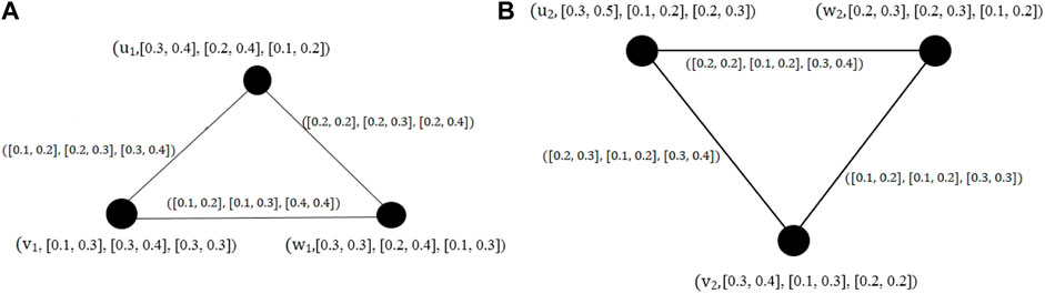
FIGURE 1. Interval-valued picture fuzzy graphs. Sets (A) and (B).
Definition 9. Let G = (C, D) be an IVPFG. Then, the degree(open degree) of a vertex u of G is
If
Definition 10. Let G = (C, D) be an IVPFG. Then, the total degree(close degree) of a vertex u is
Definition 11. Given an IVPFG G = (C, D), the order of G is defined by
Definition 12. Given an IVPFG G = (C, D), the size of G is
Example 2. Degrees of all vertices of an IVPFG shown in Figure 1A are as follows:
The total degrees of all vertices of the same IVPFG are given by
Hence, the order of G is
Definition 13. For every two IVPFGs G = (C 1, D 1) and H = (C 2, D 2), the union and intersection can be defined as follows.
(1) Union:
where
Then, we have the following.
and
Proposition 1. The union of two IVPFGs G = (C 1, D 1) and H = (C 2, D 2) is an IVPFG.
Proof. Let wx ∈ E 1 ∩ E 2. Then,
(1)
(2)
(3)
Similarly, if wx ∈ E 1 and wx ∈ E 2 or wx ∈ E 2 and wx ∈ E 1, then we have
Definition 14. The complement of an IVPFG H = (C, D) is an IVPFG H c = (C c , D c ) if and only if it obeys
for all x ∈ V. In addition, for all wx ∈ E,
Example 3. Graphs shown in Figure 2 are the complement of each other.
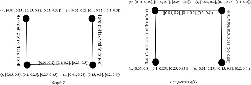
FIGURE 2. Complement of an interval-valued picture fuzzy graph.
Definition 15. Let G* = (C, D) be an IVPFG on G = (V, E), where C =
where χ IL (w, x) ≤ χ DL (w, x), χ IU (w, x) ≤ χ DU (w, x), ψ IL (w, x) ≤ ψ DL (w, x), ψ IU (w, x) ≤ ψ DU (w, x), ω IL (w, x) ≥ ω DL (w, x), ω IU (w, x) ≥ ω DU (w, x).
Definition 16. An IVPFG H = (C, D) is a regular IVPFG, if
∑ w, w≠x χ DL (w, x) = constant, ∑ w, w≠x χ DU (w, x) = constant
∑ w, w≠x ψ DL (w, x) = constant, ∑ w, w≠x ψ DU (w, x) = constant
∑ w, w≠x ω DL (w, x) = constant, and ∑ w, w≠x ω DU (w, x) = constant.
Example 4. It is easy to conclude that the graph given in Figure 3 is a regular IVPFG.
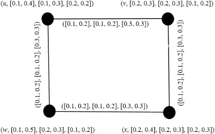
FIGURE 3. Regular interval-valued picture fuzzy graph.
Definition 17. An IVPFG H = (C, D), where
∀ (w, x) ∈ E.
Definition 18. An IVPFG H = (C, D), where C = ([χ CL , χ CU ], [ψ CL , ψ CU ], [ω CL , ω CU ]) and D = ([χ DL , χ DU ], [ψ DL , ψ DU ], [ω DL , ω DU ]) is said to be a complete IVPFG if H satisfies
∀ w, x ∈ V.
Example 5. The graph shown in Figure 4 is a complete IVPFG.
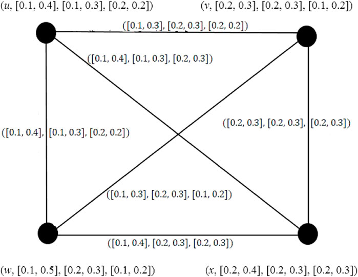
FIGURE 4. Complete interval-valued picture fuzzy graph.
Remark 1. Every complete IVPFG is a strong IVPFG, but the converse is not true, in general.
Definition 19. Let E
1 be an IVPFR on (V
1 × V
1) and E
2 be an IVPFR on (V
2 × V
2). Then, the max–min composed relation (IVPCR) is an IVPFR on (V
1 × V
2) and is described as
Definition 20. The composition G[H] = (C 1◦C 2, D 1◦D 2) of two IVPFGs G = (C 1, D 1) and H = (C 2, D 2) is defined as follows:
1.
2.
for all x ∈ V 1 and x 2 y 2 ∈ E 2
3.
for all z ∈ V 2 and x 1 y 1 ∈ E 1
4.
for all x 2 y 2 ∈ V 2, x 2 ≠ y 2 and ∀(x 1 y 1) ∈ E 1
5.
6.
for all x ∈ V 1 and x 2 y 2 ∈ E 2
7.
for all z ∈ V 2 and x 1 y 1 ∈ E 1
8.
for all x 2 y 2 ∈ V 2, x 2 ≠ y 2 and ∀(x 1 y 1) ∈ E 1
9.
10.
for all x ∈ V 1 and x 2 y 2 ∈ E 2
11.
for all z ∈ V 2 and x 1 y 1 ∈ E 1
12.
for all x 2 y 2 ∈ V 2, x 2 ≠ y 2 and ∀(x 1 y 1) ∈ E 1
Proposition 2. Let G and H be two IVPFGs defined on G* and H*, respectively. Then, their composition is an IVPFG on G*[H*].
Proof. The proof is similar to that of Proposition 1; we only prove the condition for D
1◦D
2. In the case w
1 ∈ V
1, w
2
v
2 ∈ E
2, by Proposition 1
(A)
Again, for all y 2 ∈ V 2 and w 1 x 1 ∈ E 1, we have
(B)
Similarly, for all y 2 ∈ V 2 and w 1 x 1 ∈ E 1, we have
(C)
Similarly, for all y 2 ∈ V 2 and w 1 x 1 ∈ E 1, we have
Definition 21. Let
(A)
(B)
(C)
Proposition 3. Let
Proof. We only provide the proof about D 1 × D 2, and the condition for C 1 × C 2 is evident. Let w 1 ∈ V 1, w 2 x 2 ∈ E 2. Then,
(a)
Similarly, for all y 2 ∈ V 2 and w 1 x 1 ∈ E 1, we have
(b)
Similarly, for all y 2 ∈ V 2 and w 1 x 1 ∈ E 1, we have
(c)
Similarly, for all y 2 ∈ V 2 and w 1 x 1 ∈ E 1, we have
Definition 22. Let G* = (C
1, D
1) and
(A)
and
(B)
and
(C)
and
where wx is the edge between the vertices w and x, and E 1, and E 2 are the edges sets of the graphs G* and G**, respectively.
Theorem 1. Ring sum of any two IVPFGs is an IVPFG.
We provide Example 7 in support of Theorem 1.
Example 6. From Figure 5, it is easy to check that G* ⊕ G** is an IVPFG.
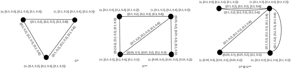
FIGURE 5. Ring sum of two interval-valued picture fuzzy graphs.
Remark 2. Let G* = (C
1, D
1) and G** = (C
2, D
2), where C
1 =
Theorem 2. Let H = (C, D), where
Proof. Results follow from the definitions of the union, intersection, and ring sum of IVPFGs.
Definition 23. Let
Example 7. By deleting an edge e = u 1 w 1 = ([0.2, 0.2], [0.2, 0.3], [0.2, 0.4]) from the graph shown in Figure 1A = H, we obtain a subgraph shown in Figure 6, which implies H − e = H ⊕ e.
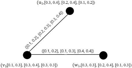
FIGURE 6. H − e = H ⊕ e.
4 Connectedness and different types of strengths of the edges of IVPFGs
Definition 24. A path p in an IVPFG G is the sequence of different vertices w
0, w
1, w
2, …, w
k
satisfying
Definition 25. Let H = (C, D) be an IVPFG. Let us consider that the two vertices w and x are connected by a path of length k in H like p: w
0, w
1, w
2, …w
k−1, w
k
. Then,
Let
Definition 26. We call an IVPFG G = (C, D).
1. A semi χ − strong if χ
DL
(w
i
w
j
) = min
2. A semi ψ − strong if ψ
DL
(w
i
w
j
) = min
3. A semi ω − strong if ω
DL
(w
i
w
j
) = max
4. Strong, if it is semi χ-strong, semi ψ-strong, and semi ω-strong
5. Complete χ − strong if χ
DL
(w
i
w
j
) = min
6. Complete ψ − strong if χ
DL
(w
i
w
j
) < min
7. Complete ω − strong if χ
DL
(w
i
w
j
) < min
8. Complete if χ
DL
(w
i
w
j
) = min
Example 8. In Figure 7, the edges (u, v), (v, x), (x, w), and (w, u) are semi χ-strong, semi ψ-strong, and semi ω-strong edges. Consequently, edges (u, v), (v, x), (x, w), and (w, u) are the strong edges.
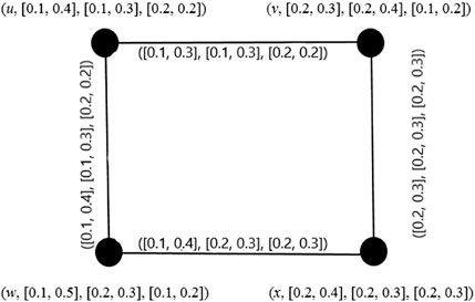
FIGURE 7. Strong = (semi χ − strong, semi ψ − strong, and semi ω − strong).
Example 9. In Figure 8, the edge (u, w) is complete χ-strong, the edge (w, x) is complete ψ-strong, the edge (u, v) is complete ω − strong, and the edge (v, x) is a complete edge.
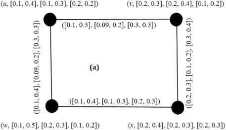
FIGURE 8. Complete χ − strong, complete ψ − strong, and complete ω − strong graph.
Theorem 3. A path P′ in an IVPFG G is the sequence of distinct vertices w 1, w 2, …, w n such that either one of the following conditions is satisfied:
(i) χ DL (w i w j ) > 0, χ DU (w i w j ) > 0, ψ DL (w i w j ) = 0, ψ DU (w i w j ) = 0 and ω DL (w i w j ) = 0, ω DU (w i w j ) = 0 for some i and j,
(ii) χ DL (w i w j ) = 0, χ DU (w i w j ) = 0, ψ DL (w i w j ) > 0, ψ DU (w i w j ) > 0 and ω DL (w i w j ) = 0, ω DU (w i w j ) = 0 for some i and j,
(iii) χ DL (w i w j ) = 0, χ DU (w i w j ) = 0, ψ DL (w i w j ) = 0, ψ DU (w i w j ) = 0 and ω DL (w i w j ) > 0, ω DU (w i w j ) > 0 for some i and j,
(iv) χ DL (w i w j ) > 0, χ DU (w i w j ) > 0, ψ DL (w i w j ) > 0, ψ DU (w i w j ) > 0 and ω DL (w i w j ) = 0, ω DU (w i w j ) = 0 for some i and j,
(v) χ DL (w i w j ) = 0, χ DU (w i w j ) = 0, ψ DL (w i w j ) > 0, ψ DU (w i w j ) > 0 and ω DL (w i w j ) > 0, ω DU (w i w j ) > 0 for some i and j,
(vi) χ DL (w i w j ) > 0, χ DU (w i w j ) > 0, ψ DL (w i w j ) = 0, ψ DU (w i w j ) = 0 and ω DL (w i w j ) > 0, ω DU (w i w j ) > 0 for some i and j, and
(vii) χ DL (w i w j ) > 0, χ DU (w i w j ) > 0, ψ DL (w i w j ) > 0, ψ DU (w i w j ) > 0 and ω DL (w i w j ) > 0, ω DU (w i w j ) > 0 for some i and j.
Proof. It is easy to verify by using the definition of the path in an IVPFG.
Definition 27. If P′ = w 1, w 2, …, w n is a path in G, then
(i) the χ-strength of path P′ is {[minχ DL (w i w j ), minχ DU (w i w j )]}, for every i, j = 1, 2, …, n, abbreviated as P χ ,
(ii) the ψ-strength of path P′ is {[minψ DL (w i w j ), minψ DU (w i w j )]}, for every i, j = 1, 2, …, n, abbreviated as P ψ , and
(iii) the ω-strength of path P′ is {[maxω DL (w i w j ), maxω DU (w i w j )]}, for every i, j = 1, 2, …, n, abbreviated as P ω .
Different types of strengths of connectedness of nodes are described as follows.
Definition 28. If w i , w j ∈ V ⊆ G. Then,
(i) the χ-strength of connectedness between the two nodes w
i
and w
j
is
(ii) the ψ-strength of connectedness between the two nodes w
i
and w
j
is
(iii) the ω-strength of connectedness between the nodes w
i
and w
j
is
of all possible paths between w i and w j .
By
Definition 29. An edge (w i , w j ) is a bridge in G, if either
OR
Alternatively, removing an edge (w i , w j ) decreases the strength of connectedness between the pair of vertices (w i , w j ) called a bridge, if there exist the vertices w i , w j with (w i , w j ) being the edge of every strongest path from w i to w j .
Definition 30. An edge (w i , w j ) in G is
(i) η-strong, if
(ii) φ-strong, if
(iii) ξ-strong, if
Remark 3. Let G be an IVPFG. Then,
(i) if all the edges in a path G are η-strong, we call it an η-strong path in G. In the φ-strong path, all the edges are φ-strong, and a path is ξ-strong if all its edges are ξ-strong;
(ii) the strongest path may contains all types of edges that are η-strong, φ-strong, and ξ-weak; and
(iii) a strong path contains only η-strong or φ-strong edges but no ξ-weak edges.
Theorem 4. An edge (w i , w j ) of an IVPFG G is a bridge if and only if it is η-strong.
Proof. Let (w i , w j ) be an IVPFB. Then,
then
Conversely, let (w i , w j ) be η-strong. By definition, w i w j is the only strongest path from w i to w j and the deletion of (w i , w j ) will reduce the strength of connectedness between w i and w j . Hence, (w i , w j ) is an IVPFB. It is notable that if an edge (w i , w j ) in G is an IVPFB, then
Remark 4. The converse of the aforementioned theorem does not hold true.
Remark 5. There exists utmost one η-strong edge in a complete IVPFG.
Theorem 5. A complete IVPFG has no ξ-edge.
Proof. Let G be a complete IVPFG. If possible, let us assume that G contains an ξ-edge (w i , w j ); then,
It means there is a stronger path P′ other than (w
i
, w
j
) from w
i
to w
j
in a graph G. Let
Theorem 6. Let G be any complete IVPFG without an η-strong edge. Let P′ be a w i w j path in G. Then, the following statements are equivalent:
(i) P′ is a strong w i w j path.
(ii) P′ is the strongest w i w j path.
Proof. (i) ⇒ (ii) Let G be a complete IVPFG without η-strong edges. Let P′ be any w i w j path in G. We assume that P′ is a strong w i w j path. By definition, all edges in G are φ-strong edges or ξ-strong edges.
(ii) ⇒ (i) Let P′ be the strongest w i w j path in G. Let the path P′ contain only φ-strong edges or ξ-strong edges, and hence, w i w j is a strong path.
5 Interval-valued picture fuzzy logic system for the TCP
The TCP is a transport protocol used on top of the Internet Protocol (IP) to ensure the reliable transmission of packets. The TCP includes mechanisms to address problems that arise due to a packet-based messaging which include lost packets, out-of-order packets, and corrupted packets. Conventional logic accepts exact inputs and yields definite outputs such as “Yes” or “No.” We can easily analyze the TCP using appropriate graphs. However, in reality, crisp graphs can only represent “Yes” or “No” values. Consequently, classical graphs cannot simultaneously detect the transmission rate in terms of received packets, lost packets, and corrupted packets. Classical graphs can only determine packet conditions after the sender sends the packets, starts a timer, and places the packets in a retransmission queue. If the timer expires without an acknowledgment from the recipient, the sender resends the packet. These re-sending data can lead to the occurrence of duplicate packets, which can cause congestion, where a packet was not genuinely lost but experienced delays in acknowledgment.
On the other hand, a fuzzy logic system (FLS) processes incomplete and inaccurate inputs to produce acceptable outputs. A fuzzy logic-based TCP can handle vague and erroneous network states effectively. However, the aforementioned circumstances of sent and received data cannot be explained using a simple FLS. Consequently, fuzzy graphs or even intuitionistic fuzzy graphs are incapable of representing the three states of packets: received, lost, and corrupted. Fortunately, this situation can be addressed accurately using IVPFGs. Through IVPFGs, we can simultaneously determine the transmission rate by detecting the rate at which packets are received, lost, and out of order (corrupted). We represent received packets, lost packets, and out-of-order packets with positive membership, negative membership, and neutral membership values, respectively (i.e., ([a, b], [c, d], [e, f])). By utilizing IVPFGs, we can enhance the fuzzy logic system presented in [47, 48] for TCP analysis. Since, the interval-valued picture fuzzy logic-based TCP includes lost and out-of-order packets, the system based on IVPFGs would be more efficient in dealing with the TCP) as compared to the TCP based on fuzzy logic described in [48].
The layout of the TCP based on IVPFSs is as follows.
In a fuzzy-based error detection mechanism (FEDM), a fuzzy logic controller (FLC) was used to distinguish congestion losses and random channel losses (losses due to wireless errors). The FEDM uses an improved error detector (IED) module to identify the possible cause of a loss. The IED output is manipulated through three flags: C—congestion, U—uncertain, and B—bit error (wireless errors). The error recovery mechanism (ERM) accepts the output of the IED and acts properly. The retransmission timeout (RTO) with congestion or uncertain (C flag is set or U flag is set) retransmits and decreases the transmission rate. When the RTO takes place due to a bit error (indicated by the B flag being set), retransmissions are performed without reducing the transmission rate. In addition to the error recovery mechanism provided by the FEDM (fast error detection and mitigation), the fast retransmission phase has the ability to autonomously identify and address the errors, and it happens when the receiver receives three duplicate acknowledgments (ACKs).
The FEDM becomes active when it receives an ACK, and the functions involve in it monitors the total number of hops and fluctuations occurring in round trip time (RTT) values through the entire network. An increase in RTT can occur due to either congestion or an increase in the number of hops. The count of hops is determined by checking time to live (TTL) field in the corresponding IP header. The RR-RTT rate module identifies intervals where the RTT increases by a value greater than α, with n representing the number of such occurrences. In [5], it was suggested that satisfactory outcomes can be achieved by setting n to [1.52.5], α to 15–25 percent, and the sampling duration between two RTT values to 100 ms. The NH information is utilized to quickly classify the input/output equipment device (IED) status as congestion if there is a significant increase in RTT without a corresponding increase in the number of hops. The input variables for this process include the mean t − RTT and the variance Δ t − RTT.
There are three sets characterized as small, medium, and large for both t and Δt. The fuzzy engine’s output is represented by three individual sets denoting congestion, bit error, and uncertain status.
The IVPF-TCP utilizes the fuzzy logic controller to calculate the value of Cwnd (congestion window), a TCP parameter that monitors the transmission rate. By taking into account the current values of Cwnd, SSThresh (slow start threshold), and RTT, it estimates the next subsequent value of Cwnd. TCP’s slow start and congestion avoidance phases demonstrate exponential and linear growth in the transmission rate, respectively. Slow start gradually increases Cwnd initially and then accelerates toward the end. In the event of packet loss, TCP halves Cwnd and transitions to congestion avoidance. Nevertheless, during transition from slow start to congestion avoidance, the possibility of packet loss may occur. The aim of fuzzy TCP is to modify the transition of the congestion window (Cwnd), achieving an improved process. The six fuzzy sets for Cw are decrease very large (DVL), decrease large (DL), decrease medium (DM), decrease small (DS), no change (NC), and increase (I) (these are elaborated in Tables 1–3). Some fuzzy rules for TCP are mentioned in Tables 1–3. Triangular membership functions are employed, with the maximum throughput that serve as the upper limit. We can represent the received packets, lost packets, and out-of-order packets by positive membership, negative membership, and neutral membership values, respectively (i.e., ([a, b], [c, d], [e, f])). The range for Cw is [−3, −1] to [0, 0.1] instead of numbers −2.0 to 0.005 as were taken in [49]. Here, we are taking the values of congestion window size (cw) [−3, −1] to [0, 0.1] instead of −2.0 to 0.005. The considered values are in intervals instead of numbers, which are encompassing the values considered in [49]. In this way, the proposed methodology is relaxing the values.
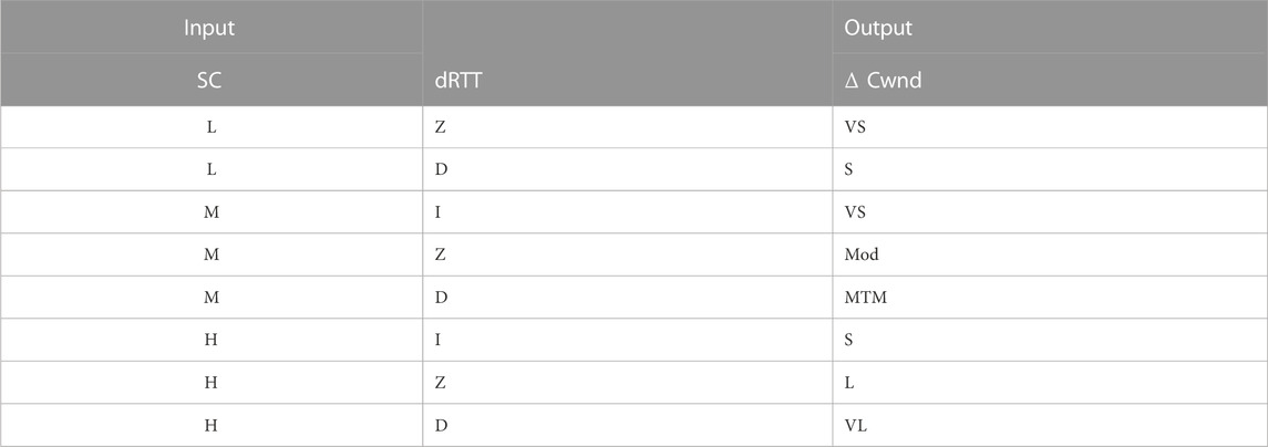
TABLE 1. [47] Interval-valued picture TCP.
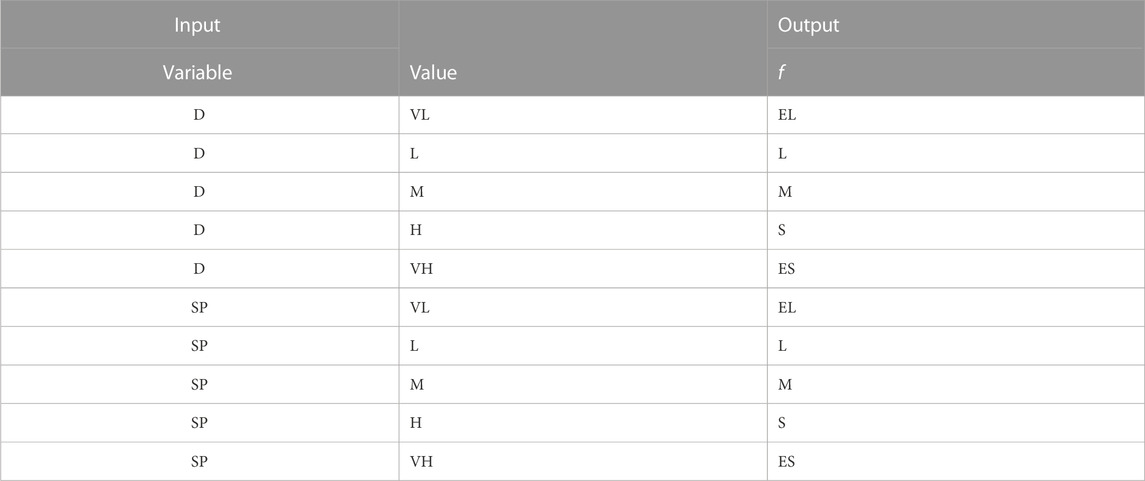
TABLE 2. [50] Interval-valued picture fuzzy rules- IVPF-based transport rules.
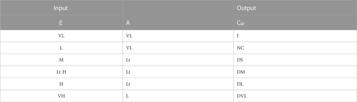
TABLE 3. [49] Interval-valued picture fuzzy rules- IVPFL-TCP.
By taking input at one node and output at the other end (vertex) of the IVPFG and the other way around, we can manipulate the situation very easily. The simulation can be executed in NS-2 simulator, and we can get more adequate enhancement in performance in terms of throughput and the packet delay.
Description: Here, VS—very small, S—small, ES—extreme small, M—medium, H—high, Mod—moderate, MTM—more than moderate, VS—very small, S—small, L—large, VL—very large, EL—extreme large, VH—very high, and LT—little high.
6 Application of IVPFGs toward social networking
IVPFGs are the best to deal different social networks such as Instagram, Facebook, WhatsApp, TikTok, and Twitter. In these networks, we can consider the individual or a group of people or might be any organization as node, while their relationships (if exist) can be depicted through edges between the nodes. Since there are variations in relationships, we can consider a node (a person, organization, etc.) has good, not good, and no (neutral) activities. Then, the degrees of good, not good, and no activities of the nodes can be represented in terms of subintervals of [0, 1]. Similarly, the degrees of the relationships among nodes measure the edge membership values. It has been observed that the two persons have good attitude for some types of activities (such as exam structure and paper organization), they can have no good mind for some other types of activities (religion, food habit, etc.) while they do not have any activity toward business. Thus, there are three types of edge membership values such as good, bad, and neutral. Thus, such type of networks can be best manipulated through IVPFGs.
7 Conclusion
The theory of fuzzy graphs provides an effective tool to model the uncertain real-world problems in various fields of science, including computer science, information technology, decision-making theory, statistics, and pattern recognition. Several generalizations of fuzzy graphs have been explored in order to handle such types of complex real-life problems. An IVPFS is a direct extension of the IVFS and PFS. While discussing IVPFGs in this manuscript, we introduce the notion of IVPFGs, which is an extension of both IVFGs and PFGs. We utilize the concepts of interval-valued picture fuzzy relations to define IVPFGs. First, for investigation purposes, we apply different types of operations to IVPFGs, including the ring sum of two IVPFGs. We introduce special types of IVPFGs such as complete IVPFGs, regular IVPFGs, strong IVPFGs, and complement IVPFGs. Additionally, we explore different product types of IVPFGs, such as Cartesian product and direct product. We introduce and apply different strengths of paths, such as strong, semi-strong, and complete strong, to analyze the connectivity of IVPFGs. Furthermore, we explore structural properties of IVPFGs through these arcs. Since PFSs have an additional degree called neutrality compared to intuitionistic fuzzy sets, they prove to be a more efficient tool for expressing uncertainties. Consequently, IVPFGs are more efficient in modeling real-life problems containing uncertainties compared to other forms of fuzzy graphs. At the end, we provide a clue as an application of IVPFGs toward the TCP and plan to write a full-length article on the TCP based on IVPFGs. Moreover, we also provided the application of IVPFGs toward social networks. Furthermore, IVPFGs can be utilized in other fields of sciences such as image processing, database systems, social networks, and transportation networks. In spite of all these, one could shift this study toward bipolar picture fuzzy graphs.
Data availability statement
The raw data supporting the conclusion of this article will be made available by the authors, without undue reservation.
Author contributions
XS: conceptualization, funding acquisition, investigation, project administration, validation, writing–original draft, and writing–review and editing. SK: conceptualization, investigation, project administration, supervision, validation, visualization, writing–original draft, and writing–review and editing. WK: conceptualization, formal analysis, methodology, validation, writing–original draft, and writing–review and editing.
Funding
The authors declare that financial support was received for the research, authorship, and/or publication of this article. This work was supported by the National Key R & D Program of China (grant no. 2019YFA0706402) and the National Natural Science Foundation of China under (grant nos. 62172302, 62072129, and 61876047).
Conflict of interest
The authors declare that the research was conducted in the absence of any commercial or financial relationships that could be construed as a potential conflict of interest.
Publisher’s note
All claims expressed in this article are solely those of the authors and do not necessarily represent those of their affiliated organizations, or those of the publisher, the editors, and the reviewers. Any product that may be evaluated in this article, or claim that may be made by its manufacturer, is not guaranteed or endorsed by the publisher.
References
2. Zadeh LA. The concept of a linguistic variable and its application to approximate reasoning—I. Inf Sci (1975) 8:199–249. doi:10.1016/0020-0255(75)90036-5
3. Turksen IB. Interval valued fuzzy sets based on normal forms. Fuzzy sets Syst (1986) 20:191–210. doi:10.1016/0165-0114(86)90077-1
4. Gorzałczany MB. A method of inference in approximate reasoning based on interval valued fuzzy sets. Fuzzy sets Syst (1987) 21:1–17. doi:10.1016/0165-0114(87)90148-5
5. Gorzałczany MB. An interval valued fuzzy inference method some basic properties. Fuzzy Sets Syst (1989) 31:243–51. doi:10.1016/0165-0114(89)90006-7
6. Atanassov K. Intuitionistic fuzzy sets. Fuzzy Sets Syst (1986) 20:87–96. doi:10.1016/s0165-0114(86)80034-3
7. Li DF. Multiattribute decision making models and methods using intuitionistic fuzzy sets. J Comput Syst Sci (2005) 70:73–85. doi:10.1016/j.jcss.2004.06.002
8. Chaira T, Ray AK. A new measure using intuitionistic fuzzy set theory and its application to edge detection. Appl soft Comput (2008) 8:919–27. doi:10.1016/j.asoc.2007.07.004
9. Atanassov KT, Atanassov KT. Interval valued intuitionistic fuzzy sets. Intuitionistic fuzzy sets: Theor Appl (1999) 139–77.
11. Phong PH, Hieu DT, Ngan R, Them PT. Some compositions of picture fuzzy relations. In: Proceedings of the 7th national conference on fundamental and applied information technology research (FAIR7). Thai Nguyen (2014). p. 19–20.
12. Cuong BC, Pham VH. Some fuzzy logic operators for picture fuzzy sets. In: 2015 seventh international conference on knowledge and systems engineering. (KSE) (IEEE) (2015). p. 132–7.
13. Wei G. Some cosine similarity measures for picture fuzzy sets and their applications to strategic decision making. Informatica (2017) 28:547–64. doi:10.15388/informatica.2017.144
14. Saad M, Rafiq A, Perez-Dominguez L. Methods for multiple attribute group decision making based on picture fuzzy dombi hamy mean operator. J Comput Cogn Eng (2022). doi:10.47852/bonviewjcce2202206
15. Kumar S, Garg H. Some novel point operators and multiple rounds voting process based decision-making algorithm under picture fuzzy set environment. Adv Eng Softw (2022) 174:103274. doi:10.1016/j.advengsoft.2022.103274
16. Khalil AM, Li SG, Garg H, Li H, Ma S. New operations on interval valued picture fuzzy set, interval valued picture fuzzy soft set and their applications. Ieee Access (2019) 7:51236–53. doi:10.1109/access.2019.2910844
17. Khan WA, Faiz K, Taouti A. Bipolar picture fuzzy sets and relations with applications. Songklanakarin J Sci Technol (2022) 44.
18. Rosenfeld A. Fuzzy graphs. Fuzzy sets and their applications to cognitive and decision processes . Elsevier (1975). p. 77–95.
20. Sunitha M, Vijayakumar A. Complement of a fuzzy graph. Indian J Pure Appl Maths (2002) 33:1451–64.
21. Shoaib M, Kosari S, Rashmanlou H, Malik MA, Rao Y, Talebi Y, et al. Notion of complex pythagorean fuzzy graph with properties and application. J Multiple-Valued Logic Soft Comput (2020) 34.
22. Samanta S, Sarkar B, Shin D, Pal M. Completeness and regularity of generalized fuzzy graphs. SpringerPlus (2016) 5:1979–14. doi:10.1186/s40064-016-3558-6
23. Rashmanlou H, Samanta S, Pal M, Borzooei RA. Intuitionistic fuzzy graphs with categorical properties. Fuzzy Inf Eng (2015) 7:317–34. doi:10.1016/j.fiae.2015.09.005
24. Mandal S, Sahoo S, Ghorai G, Pal M. Genus value of m-polar fuzzy graphs. J Intell Fuzzy Syst (2018) 34:1947–57. doi:10.3233/jifs-171442
25. Ghorai G, Pal M. Some isomorphic properties of m-polar fuzzy graphs with applications. SpringerPlus (2016) 5:2104–21. doi:10.1186/s40064-016-3783-z
26. Akram M, Dudek WA. Interval-valued fuzzy graphs. Comput Maths Appl (2011) 61:289–99. doi:10.1016/j.camwa.2010.11.004
27. Rashmanlou H, Jun YB, Borzooei R. More results on highly irregular bipolar fuzzy graphs. Ann Fuzzy Maths Inform (2014) 8:149–68.
28. Rehman FU, Rashid T, Hussain MT. Optimization in business trade by using fuzzy incidence graphs. J Comput Cogn Eng (2022). doi:10.47852/bonviewjcce2202176
29. Shannon A, Atanassov KT. A first step to a theory of the intuitionistic fuzzy graphs. In Proc. of the First Workshop on Fuzzy Based Expert Systems (D. akov, Ed.), Sofia (1994) pp. 59–61.
30. Shannon A, Atanassov K. On a generalization of intuitionistic fuzzy graphs. NIFS (2006) 12:24–9.
31. Thilagavathi S, Parvathi R, Karunambigai M. Operations on intuitionistic fuzzy graphs ii. International Journal of computer application (2009).
32. Akram M. Decision making method based on spherical fuzzy graphs. Decis Making Spherical Fuzzy Sets: Theor Appl (2021) 153–97.
33. Akram M, Akmal R. Operations on intuitionistic fuzzy graph structures. Fuzzy Inf Eng (2016) 8:389–410. doi:10.1016/j.fiae.2017.01.001
34. Sahoo S, Pal M. Different types of products on intuitionistic fuzzy graphs. Pac Sci Rev A: Nat Sci Eng (2015) 17:87–96. doi:10.1016/j.psra.2015.12.007
35. Shao Z, Kosari S, Rashmanlou H, Shoaib M. New concepts in intuitionistic fuzzy graph with application in water supplier systems. Mathematics (2020) 8:1241. doi:10.3390/math8081241
36. Rashmanlou H, Borzooei R, Samanta S, Pal M. Properties of interval valued intuitionistic (s,t)–fuzzy graphs. Pac Sci Rev A: Nat Sci Eng (2016) 18:30–7.
37. Qiang X, Kosari S, Chen X, Talebi AA, Muhiuddin G, Sadati SH. A novel description of some concepts in interval-valued intuitionistic fuzzy graph with an application. Adv Math Phys (2022) 2022:1–15. doi:10.1155/2022/2412012
38. Talebi AA, Rashmanlou H, Sadati SH. Interval-valued intuitionistic fuzzy competition graph. J Multiple-Valued Logic Soft Comput (2020) 34.
39. Zuo C, Pal A, Dey A. New concepts of picture fuzzy graphs with application. Mathematics (2019) 7:470. doi:10.3390/math7050470
40. Das S, Ghorai G. Analysis of road map design based on multigraph with picture fuzzy information. Int J Appl Comput Maths (2020) 6:57–17. doi:10.1007/s40819-020-00816-3
41. Das S, Ghorai G, Pal M. Certain competition graphs based on picture fuzzy environment with applications. Artif intelligence Rev (2021) 54:3141–71. doi:10.1007/s10462-020-09923-5
42. Khan WA, Ali B, Taouti A. Bipolar picture fuzzy graphs with application. Symmetry (2021) 13:1427. doi:10.3390/sym13081427
43. Khan WA, Taouti A. Dominations in bipolar picture fuzzy graphs and social networks. Results Nonlinear Anal (2023) 6:60–74.
44. Khan WA, Faiz K, Taouti A. Cayley picture fuzzy graphs and interconnected networks. Intell Autom Soft Comput (2022) 35:3317–30.
45. Chen Z, Khan WA, Khan A. Concepts of picture fuzzy line graphs and their applications in data analysis. Symmetry (2023) 15:1018. doi:10.3390/sym15051018
46. Arif W, Khan WA, Rashmanlou H, Khan A, Muhammad A. Multi attribute decision-making and interval valued picture (s,t)-fuzzy graphs. J Appl Maths Comput (2023) 69:2831–56. doi:10.1007/s12190-023-01862-y
47. Nejad HV, Yaghmaee MH, Tabatabaee H. Fuzzy tcp: optimizing tcp congestion control. 2006 Asia-Pacific Conference on Communications (IEEE) (2006), 1–5.
48. Molia HK, Kothari AD. Fuzzy logic systems for transmission control protocol. In: Proceedings of the 2nd International Conference on Communication, Devices and Computing: ICCDC 2019. Springer (2019). p. 553–65.
49. Tabash IK, Beg MS, Ahmad N. Fl-tcp: a fuzzy logic based scheme to improve tcp performance in manets. In: 2011 International Conference on Multimedia, Signal Processing and Communication Technologies. IEEE (2011). p. 188–91.
Keywords: IVPFGs, ring sum of IVPFGs, edge deletion in IVPFGs, strengths of arcs, path sequence, connectedness
Citation: Shi X, Kosari S and Khan WA (2023) Some novel concepts of interval-valued picture fuzzy graphs with applications toward the Transmission Control Protocol and social networks. Front. Phys. 11:1260785. doi: 10.3389/fphy.2023.1260785
Received: 18 July 2023; Accepted: 02 October 2023;
Published: 30 October 2023.
Edited by:
Olaniyi Samuel Iyiola, Clarkson University, United StatesReviewed by:
Said Broumi, University of Hassan II Casablanca, MoroccoMadhumangal Pal, Vidyasagar University, India
Copyright © 2023 Shi, Kosari and Khan. This is an open-access article distributed under the terms of the Creative Commons Attribution License (CC BY). The use, distribution or reproduction in other forums is permitted, provided the original author(s) and the copyright owner(s) are credited and that the original publication in this journal is cited, in accordance with accepted academic practice. No use, distribution or reproduction is permitted which does not comply with these terms.
*Correspondence: Saeed Kosari, saeedkosari38@gzhu.edu.cn