A routing strategy for spatial networks based on harmonic centrality
 Hong Lin
 Yongxiang Xia
 Xingyi Li
 Xiaoxu Gao
- School of Communication Engineering, Hangzhou Dianzi University, Hangzhou, China
With the rapid development of networks, the traffic in the networks has increased sharply, resulting in frequent congestion, especially in spatial networks, such as the railway network, aviation network, and sensor network, and congestion not only affects the user’s experience but also causes serious economic losses. Therefore, in this paper, we effectively identify the high-load nodes in spatial networks by considering harmony centrality and degree. On this basis, we design the HD routing strategy by avoiding these key nodes, which can enhance the traffic throughput of spatial networks efficiently. The results provide new ideas and directions for the design of routing strategies for spatial networks.
1 Introduction
At the end of the 20th century, the discoveries of the small-world phenomenon [1] and scale-free property [2] attracted much attention. Since then, complex networks have become a research hotspot in many fields, including communication, transportation, power grids, and social relations [3–13]. Many complex systems can be modeled into complex networks, for example, in some complex systems with transmission as their main function, such as communication networks, internet, and transport network. The constituent elements of these systems can be abstracted as nodes, and links can be used to describe the interrelationships between different elements, which can help us analyze traffic dynamics on these systems effectively. Among them, congestion is the most critical problems of such complex networks, which is related to network topology [14] and routing strategy [15]. However, it is too expensive to modify the network structure. Therefore, optimizing the routing strategy seems to be more practical to improve network transmission performance.
The shortest path (SP) routing strategy is the most common routing strategy, which is extensively adopted in various complex systems. However, it is easy to cause congestion at some hub nodes. To solve this problem, many efficient routing strategies have been proposed to avoid these hub nodes [16–26]. Yan et al. [24] realized the influence of network topology on traffic dynamics. They focused on the node degree and proposed an efficient routing strategy, which can enhance the network throughput more than 10 times. Jiang et al. [25] found that nodes with the largest betweenness are most likely to be congested, so they designed an IE strategy. The load can avoid these high-betweeness nodes during transmission, which can achieve high network throughput. Zhang et al. [26] considered both static and dynamic information and proposed an adaptive routing strategy. The load can select the appropriate path for transmission based on the waiting time and degree, which can reduce congestion effectively.
However, most current works ignore the influence of a space factor. In fact, aviation networks [27], transportation networks [28], wireless sensor networks [29], and swarming networks [30] are all limited by spatial locations. In these networks, each node has a fixed spatial location, and link length is limited. We generally call these networks as spatial networks, which is a significant class of complex networks [31]. Due to the limitation of link length, the topological structure in spatial networks is quite different with topological networks. At the same time, the traffic dynamics on spatial networks will also vary due to distinct structures [32]. For example, in the topological networks, the node degrees often exhibit an obvious power-law relationship with the loads when adopting the SP routing strategy. However, Lin et al. [33] found that this power-law relationship is not obvious in spatial networks. Most of the existing routing strategies cannot achieve great results in spatial networks. Thus, there is an urgent need for an efficient routing strategy to alleviate congestion of spatial networks.
In this paper, we focus on traffic dynamics for spatial networks. Based on the harmony centrality and degree, we redefine the key nodes in the transmission. We find that the node with the high harmony centrality index and degree usually deals with more loads. Therefore, we design a harmony-degree (HD) routing strategy to bypass these key nodes. All simulations are made on the local-area and energy-efficient (LAEE) evolution model and improved the random geometric graph (IRGG) model, which are two spatial networks with different structures. According to the results of simulation, our HD routing strategy can help spatial networks obtain greater traffic throughput.
The outline of this paper is as follows. In Section 2, we describe the generation of spatial networks. In Section 3, we explain the traffic dynamic model. In Section 4, we introduce our HD routing strategy. Simulation results and discussions are given in Section 5. In Section 6, we summarize the conclusion of this paper.
2 Network models
It has been shown that the network structure is an important factor affecting load transmission. For an efficient routing strategy, it should ensure high performance on different spatial networks. Therefore, we will test the performance of the proposed routing strategy on two spatial networks with homogeneous and heterogeneous properties, respectively. The generation of these two models is as follows.
2.1 IRGG model
The IRGG model is a simple homogeneous spatial network, which has a uniform degree distribution.
The generation process of the IRGG model is as follows:
Step 1: N nodes are distributed randomly in the 1 × 1 square area S.
Step 2: We set a connection radius r for each node. As shown in Figure 1, any node i only can establish links with nodes located in its circular connected area. The set of these nodes can be represented by Ωi.
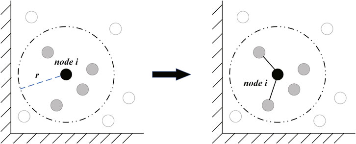
FIGURE 1. Node i build links with nodes in the set Ωi with probability p.
Step 3: We set a connection probability p. Node i establishes links with the nodes in the set Ωi with probability p.
Step 4: We repeat Step 3 until all nodes follow this rule to build links with nodes within their respective connected areas.
2.2 LAEE model
The study found that many practical networks follow the scale-free property. To explore the applicability of our proposed routing strategy on heterogeneous spatial networks, we adopt the LAEE evolution model proposed by Jiang et al. [34], which builds a spatial network with a power-law degree distribution.
The generation process of the LAEE evolution model is as follows [34]:
Step 1: N nodes are distributed randomly in the 1 × 1 square region S.
Step 2: We define the node closest to the origin as the sink node. At this point, all nodes are isolated. We set every node with the same connection radius r. If the scatter node A lies within the connection radius of node B, we call the scatter node A as the potential neighbor node of the node B.
Step 3: Sink node builds link with m0 potential neighbor nodes to form the initial network.
Step 4: At time step i, we calculate the number of potential neighbor nodes owned by different nodes in the network separately. Next, we select the one with the most network and name it as node v. Then, we select one of its potential neighbor nodes randomly and call it as node n.
Step 5: As shown in Figure 2, the node n establishes links with m nodes in the network with the priority probability Πi:
where the local-area is the set of node n’s potential neighbor nodes. kmax represents the upper limit that the node’s degree is allowed to reach, q indicates the number of nodes whose degrees arrive at kmax, and φ(E) is a function. In this paper, we set φ(Ei) = 1 and φ(Ej) = 1.
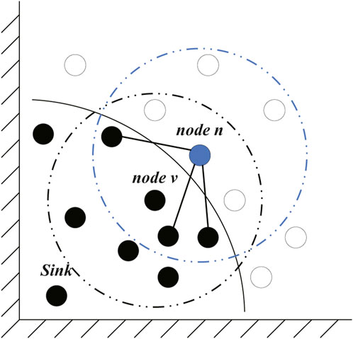
FIGURE 2. At every time step, node n builds links with nodes in the network.
Step 6: We repeat Step 4 and Step 5 until all nodes are connected to the network.
Based on the aforementioned generation methods, we can generate these two networks and observe the degree distribution. As shown in Figure 3, the degree distribution of the IRGG model is relatively even, but the LAEE model presents power-law distribution. Then, the IRGG model is a homogeneous spatial network and LAEE belongs to a heterogeneous spatial network.
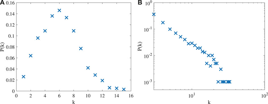
FIGURE 3. Degree distribution of the (A) IRGG network and (B) LAEE network. Parameters of the network are set as N = 1000, average degree
3 Traffic dynamics
At every time step, every node can handle at most C units of load, and R units of load are generated in the whole system. We can randomly select pairs of nodes as the sources and destinations. At each time step, we select a neighbor node as the next hop for the load according to the routing strategy. Once the load arrives at its destination, it will disappear automatically. To better understand congestion, we shall introduce the order parameter [35] as follows:
where W(t) is denoted as the units of load in the network at time t and
When R is small, the inflow and outflow of a node are balanced and no congestion occurs in the network, so η(R) = 0. We generally call this state as the free-flow state. However, with the increase of R, some load cannot be processed in time. At that time, η(R) > 0, and the congestion occurs. We always use the critical value Rc to describe this phase transition. When R < Rc, the network is in a free-flow state; when R > Rc, congestion occurs. We call Rc as the maximum network throughput. In this paper, our main work is to design an efficient routing strategy to help the spatial network obtain a higher value of throughput.
Betweeness is a significant indicator to describe the load of nodes. The betweeness of node n is calculated as follows:
where σst is the number of paths from node s to node t according to the adopted routing strategy and σst(n) represents the number of paths from node s to node t through node n. Traffic congestion first occurs at the node with maximum betweeness. In addition, the throughput of the network can be calculated by
where bmax is the maximum betweeness in the network. Therefore, in order to enhance the throughput of the network, we should minimize the value of bmax.
4 Routing strategy
For any pair of nodes {s, t}, the path between them is defined as follows:
An efficient routing strategy attempts to find the optimal path to achieve a high network throughput Rc.
4.1 SP routing strategy
The shortest path means the path with the minimum number of links between two nodes. In the SP routing strategy, load can be transmitted from its source to its destination with fewer hops. However, it easily causes congestion at hub nodes and the network has a low throughput.
4.2 Degree-location routing strategy
In the topological network, Yan et al. [24] found that the node with the larger degree always has to deal with more loads. However, in the spatial network, this relationship is not that obvious. Lin et al. [33] investigated the influence of network topology on load transmission. They found that the nodes with larger links and closer to the regional center usually process more loads. Based on this idea, they proposed the degree-location (DL) routing strategy, which is presented as follows.
Nodes are distributed in a two-dimensional region. Each node has its own coordinates. We set the center of the region as C, whose coordinate is (xc, yc). For any node v, we can calculate its Euclidean distance from the center C as
where (xv, yv) represents the 2D coordinate of node v. Next, we normalize Lv to
Similarly, the normalized degree is defined as
The weight of node v is denoted as follows:
where α and β are two adjustable exponents, corresponding to degree and location, respectively.
Considering the node with a high Q value should have large load, the DL routing strategy tends to bypass these busy nodes to improve the network throughput. To perform that, the DL routing strategy attempts to use the path with the smallest sum of the Q value, i.e.,
4.3 Harmony-degree routing strategy
In 2000, Marchiori and Latora proposed the harmonic centrality [36] denoted as
where d(i, j) represents the number of hops from node i to node j. If there is no path between node i and node j, then d(i, j) = ∞. We normalize Hi as follows:
According to Eq. 11, if node i has a high harmonic centrality index, it means that this node establishes contact with other nodes through fewer hops. Therefore, this node is busy in load transmission. At the same time, degree is also a significant factor to identify high-load nodes. With the consideration of the aforementioned two factors, the node with a high harmonic centrality index and high degree should deal with high load. Next, we attempt to combine these two factors to form a new measurement as follows:
where α and β are two exponents, corresponding to degree and harmonic centrality, respectively.
Next, we investigate the load distribution in spatial networks. Figure 4 shows that this new measurement can help us easily identify the high-load nodes in the spatial networks. If the node has a high value of w, this node needs to process more loads.
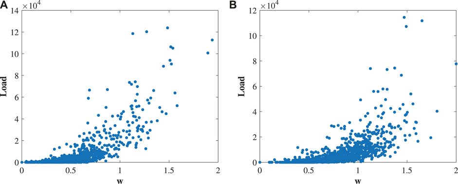
FIGURE 4. Load versus w of nodes under the shortest path (SP) routing strategy for the (A) LAEE network and (B) IRGG network with α = 1 and β = 1, respectively. Parameters of the network are set as N = 1000, average degree
In order to enhance the transmission efficiency of spatial networks, we redistribute the load from the nodes with high w to these with low. Since w depends on the harmonic centrality and degree of the node, this strategy is named as the HD routing strategy, which is defined as follows:
That is, the HD routing strategy attempts to seek a path with the minimal sum of the w value along the path.
5 Simulation results
To verify the effectiveness of HD routing strategies, we adopt Rc to measure the traffic capacity of spatial networks. If the network carries a large Rc, the congestion hardly occurs. All simulations are carried out on heterogeneous and homogeneous spatial networks, corresponding to the LAEE model and IRGG model, respectively, mentioned previously. Without the loss of generality, we set C = 1 in the following simulations.
The HD routing strategy is based on the harmonic centrality and degree, and we can use α and β to adjust their weights, respectively. Figure 5 shows the variation of Rc under different α and β. In the LAEE network, the peak value of Rc is observed at α = 1 and β = 0.6; in the IRGG network, the maximum value is observed at α = 1.4 and β = 0.5.
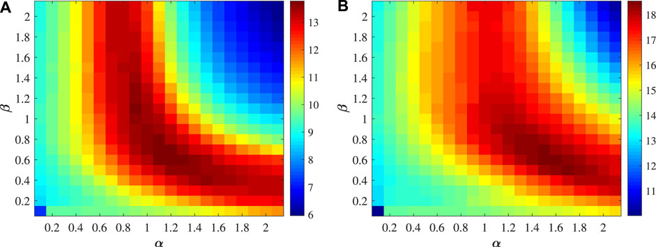
FIGURE 5. Network throughput Rc, determined by adjustable exponents α and β in the (A) LAEE network; (B) IRGG network. Parameters of the network are set as N = 1000, average degree
In order to further verify the efficiency of our routing strategy, we observe the change of Rc when adjusting the network size and average degree. In addition, we also compare with SP and DL routing strategies. Figure 6 shows the results of Rc in different scale networks. When N increases, Rc also increases. The HD strategy is always better than the SP and DL strategies in the LAEE and IRGG models.
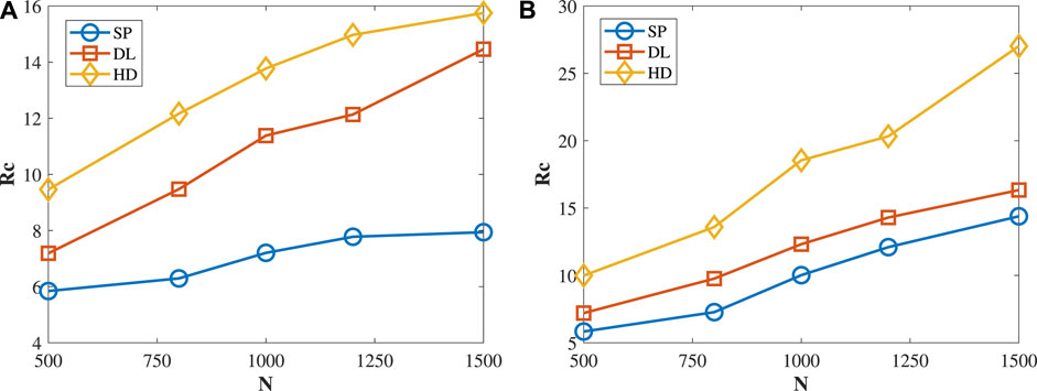
FIGURE 6. Rc of the three routing strategies on the (A) LAEE network and (B) IRGG network with different node sizes N. Parameters of the network are set as average degree
Figure 7 shows the Rc increases almost linearly with the average degree
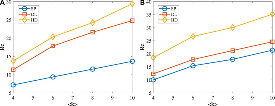
FIGURE 7. Rc of the three routing strategies on the (A) LAEE network and (B) IRGG network with different average degree
The number of hops is also an important factor to evaluate the performance of the routing strategy. As we all know, the aim of a good routing strategy is not only to enable the network to carry more load but also to allow loads to be transmitted from its source to its destination quickly. Therefore, we expect a smaller number of hops under an efficient routing strategy. Figure 8 shows the relationship between node size N and average number of hops under different routing strategies. As the name suggests, the SP routing strategy always has the minimum number of hops. In the DL strategy, the load tends to be transferred around the edge of the region. Therefore, it needs the highest number of hops.
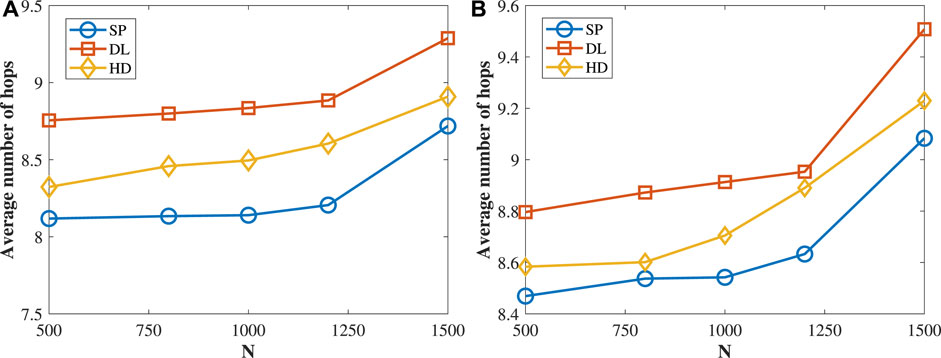
FIGURE 8. Average number of hops vs. N under three routing strategies on the (A) LAEE network and (B) IRGG network. Parameters of the network are set as average degree
Similarly, Figure 9 shows the effect of
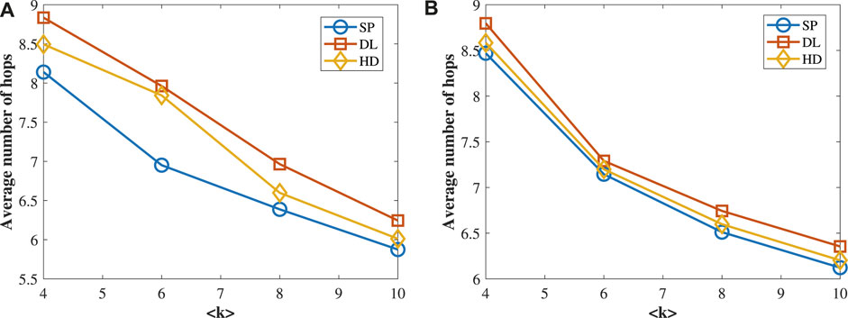
FIGURE 9. Average number of hops vs.
In order to better understand the performance of these routing strategies, we observe the average load per node under these routing strategies in different regions. As shown in Figure 10, all nodes are placed in the 1 × 1 square region S, and the region center (xc, yc) = (0.5, 0.5). S′ is a square sub-area of region S, which has the same center as the region S and side length 2d.
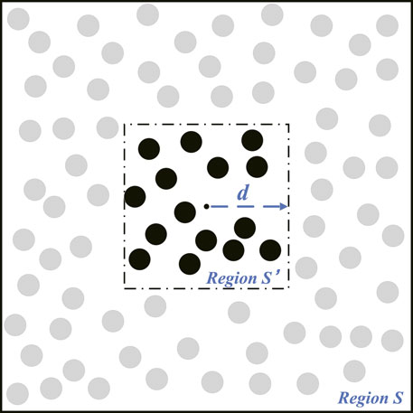
FIGURE 10. Demonstration of regions S′ and S. They have the same center (xc, yc) = (0.5, 0.5). Region S is a 1 × 1 region, and S′ is its sub-region with the side length 2d. d ≤ 0.5.
Figure 11 shows the variation of the average load per node in the region S′. When d is small, nodes in region S′ are close to the center. In this case, these nodes have high average load under the SP routing strategy. This is because the SP routing strategy finds the shortest path, which often goes through the central region. The high load leads to congestion at these nodes in the central region easily. That is why Rc is low under the SP routing strategy. On the contrary, when d is small, the average load is the lowest under the DL routing strategy. However, when d is large, the nodes need to deal with more loads under the DL routing strategy. Evidently, the load is more inclined to be transmitted along the edge of the region S. This load distribution makes the DL routing strategy always has the largest number of hops, as shown in Figures 8, 9. A high-detour cost becomes the main factor restricting the network throughput in the DL routing strategy. Compared with these two routing strategies, the load distribution is more even under the HD routing strategy. That is the main reason why the HD routing strategy performs better in spatial networks than other two routing strategies.
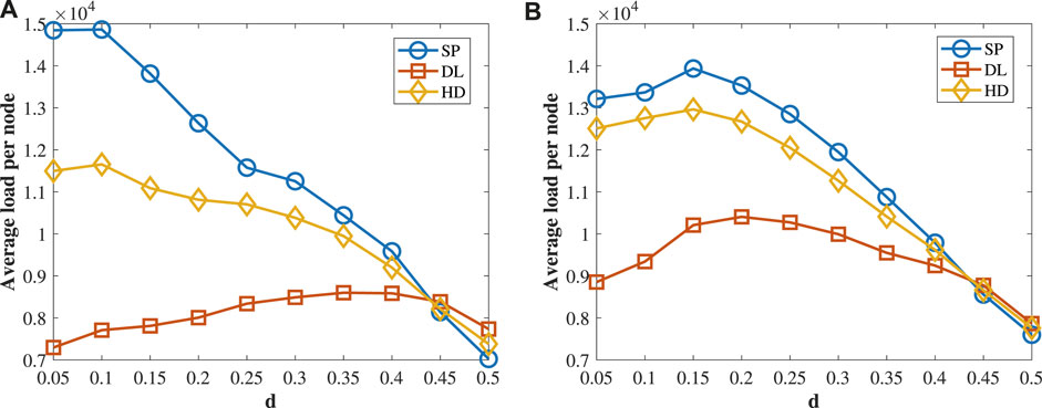
FIGURE 11. Average load per node vs. d under three routing strategies on the (A) LAEE network and (B) IRGG network. N = 1000 and r = 0.12. Center of a region is (0.5,0.5). Experimental results are the averages over 10 independent simulations.
6 Conclusion
In this paper, we design an efficient routing strategy for spatial networks. To alleviate congestion, we attempt to find high-load nodes in spatial networks. Our routing strategy redefines the high-load nodes by considering both the harmony centrality and degree to improve the throughput significantly. Moreover, it not only ensures that the network can carry more load but also ensures that the load can be quickly transmitted to the destination. Therefore, our strategy can be adopted in spatial networks to help alleviate the congestion and provide a new thought for the design of routing strategies.
Data availability statement
The original contributions presented in the study are included in the article/Supplementary Material; further inquiries can be directed to the corresponding author.
Author contributions
All authors listed have made a substantial, direct, and intellectual contribution to the work and approved it for publication.
Conflict of interest
The authors declare that the research was conducted in the absence of any commercial or financial relationships that could be construed as a potential conflict of interest.
Publisher’s note
All claims expressed in this article are solely those of the authors and do not necessarily represent those of their affiliated organizations, or those of the publisher, the editors, and the reviewers. Any product that may be evaluated in this article, or claim that may be made by its manufacturer, is not guaranteed or endorsed by the publisher.
References
1. Watts DJ, Strogatz SH. Collective dynamics of ’small-world’ networks. Nature (1998) 393:440–2. doi:10.1038/30918
2. Barabasi AL, Albert R. Emergence of scaling in random networks. Science (1999) 286:509–12. doi:10.1126/science.286.5439.509
3. Rossa FD, DeLellis P. Stochastic master stability function for noisy complex networks. Phys Rev E (2020) 101:052211. doi:10.1103/PhysRevE.101.052211
4. Huang W, Zhang T, Wei Y. Optimization for sequential communication line attack in interdependent power-communication network. Physica A (2022) 592:126837. doi:10.1016/j.physa.2021.126837
5. Tatsuro M, Yuichi I. Optimizing travel routes using temporal networks constructed from global positioning system data in kyoto tourism. Front Phys (2022) 10:1158. doi:10.3389/fphy.2022.1001983
6. Rodriguez-Sanz A, Comendador FG, Valdes RA, Perez-Castan J, Montes RB, Serrano SC. Assessment of airport arrival congestion and delay: Prediction and reliability. Transportation Res C: Emerging Tech (2019) 98:255–83. doi:10.1016/j.trc.2018.11.015
7. Liu T, Bai G, Tao J, Zhang YA, Fang Y, Xu B. Modeling and evaluation method for resilience analysis of multi-state networks. Reliability Eng Syst Saf (2022) 226:108663. doi:10.1016/j.ress.2022.108663
8. Ferenc M, Takashi N, Motter AE. Asymmetry underlies stability in power grids. Nat Commun (2021) 12:1457. doi:10.1038/s41467-021-21290-5
9. Liang Y, Xia Y, Yang X. Hybrid-radius spatial network model and its robustness analysis. Physica A (2022) 591:126800. doi:10.1016/j.physa.2021.126800
10. Zou Y, Li H. Study on power grid partition and attack strategies based on complex networks. Front Phys (2022) 9:790218. doi:10.3389/fphy.2021.790218
11. Zhou F, Lu L, Mariani MS. Fast influencers in complex networks. Commun Nonlinear Sci Numer Simulation (2019) 74:69–83. doi:10.1016/j.cnsns.2019.01.032
12. Wang Y, Li H, Zhang L, Zhao L, Li W. Identifying influential nodes in social networks: Centripetal centrality and seed exclusion approach. Chaos, Solitons and Fractals (2022) 162:112513. doi:10.1016/j.chaos.2022.112513
13. Das K, Samanta S, Pal M. Study on centrality measures in social networks: A survey. Social Netw Anal Mining (2018) 8:13–1. doi:10.1007/s13278-018-0493-2
14. Mohseni A, Gharibzadeh S, Bakouie F. The effect of network structure on desynchronization dynamics. Commun Nonlinear Sci Numer Simulation (2018) 63:271–9. doi:10.1016/j.cnsns.2018.02.011
15. Tan F, Wu J, Xia Y, Tse CK. Traffic congestion in interconnected complex networks. Phys Rev E (2014) 89:062813. doi:10.1103/PhysRevE.89.062813
16. Echague J, Cholvi V, Kowalski DR. Effective use of congestion in complex networks. Physica A (2018) 494:574–80. doi:10.1016/j.physa.2017.11.159
17. Ling X, Wang X, Chen J, Liu D, Zhu K, Guo N. Major impact of queue-rule choice on the performance of dynamic networks with limited buffer size. Chin Phys B (2020) 29:018901. doi:10.1088/1674-1056/ab5935
18. Kirst C, Timme M, Battaglia D. Dynamic information routing in complex networks. Nat Commun (2016) 7:11061. doi:10.1038/ncomms11061
19. Wang C, Xia Y, Zhu L. A method for identifying the important node in multi-layer logistic networks. Front Phys (2016) 10:968645. doi:10.3389/fphy.2022.968645
20. Dong T, Hu W, Liao X. Dynamics of the congestion control model in underwater wireless sensor networks with time delay. Chaos, Solitons and Fractals (2016) 92:130–6. doi:10.1016/j.chaos.2016.09.019
21. Ohnishi M, Minamiguchi C, Ohsaki H. In: WK Chan, B Claycomb, H Takakura, JJ Yang, YT amd Dave Towey, S Seguraet al. editors. On the performance of end-to-end routing in complex networks with intermittent links. 2020 IEEE 44th annual computers, software, and applications conference (COMPSAC). IEEE) (2020). p. 1157–62.
22. Almasan P, Suarez-Varela J, Rusek K, Barlet-Ros P, Cabellos-Aparicio A. Deep reinforcement learning meets graph neural networks: Exploring a routing optimization use case. Comput Commun (2016) 196:184–94. doi:10.1016/j.comcom.2022.09.029
23. Ma J, Wei J, Tang X, Zhao X. An improved efficient routing strategy on two-layer networks. Pramana (2022) 96:95. doi:10.1007/s12043-022-02344-9
24. Yan G, Zhou T, Hu B, Fu Z, Wang B. Efficient routing on complex networks. Phys Rev E (2006) 73:046108. doi:10.1103/PhysRevE.73.046108
25. Jiang Z, Liang M. Improved efficient routing strategy on scale-free networks. Int J Mod Phys C (2012) 23:1250016. doi:10.1142/S0129183112500167
26. Zhang H, Liu Z, Tang M, Hui P. An adaptive routing strategy for packet delivery in complex networks. Phys Lett A (2007) 364:177–82. doi:10.1016/j.physleta.2006.12.009
27. Donnet T, Ryley T, Lohmann G, Spasojevic B. Developing a queensland (Australia) aviation network strategy: Lessons from three international contexts. J Air Transport Manage (2018) 73:1–14. doi:10.1016/j.jairtraman.2018.08.003
28. Wang Y, Wu Q, Song J. Spatial network structure characteristics of green total factor productivity in transportation and its influencing factors: Evidence from China. Front Environ Sci (2022) 10:982245. doi:10.3389/fenvs.2022.982245
29. Li J, Wang Z, Lu R, Xu Y. Partial-nodes-based state estimation for complex networks with constrained bit rate. IEEE Trans Netw Sci Eng (2021) 8:1887–99. doi:10.1109/TNSE.2021.3076113
30. Xu B, Bai G, Liu T, Fang Y, an Zhang Y, Tao J. An improved swarm model with informed agents to prevent swarm-splitting. Chaos, Solitons and Fractals (2023) 169:113296. doi:10.1016/j.chaos.2023.113296
32. Xia Y, Wang C, Shen HL, Song H. Cascading failures in spatial complex networks. Physica A (2020) 559:125071. doi:10.1016/j.physa.2020.125071
33. Lin H, Xia Y, Liang Y. Efficient routing for spatial networks. Chaos: Interdiscip J Nonlinear Sci (2022) 32:053110. doi:10.1063/5.0091976
34. Jiang L, Jin X, Xia Y, Ouyang B, Wu D, Chen X. A scale-free topology construction model for wireless sensor networks. Int J Distributed Sensor Networks (2014) 10:764698. doi:10.1155/2014/764698
35. Arenas A, Díaz-Guilera A, Guimerà R. Communication in networks with hierarchical branching. Phys Rev Lett (2001) 86:3196–9. doi:10.1103/PhysRevLett.86.3196
Keywords: spatial networks, routing strategy, harmony centrality, congestion, complex network
Citation: Lin H, Xia Y, Li X and Gao X (2023) A routing strategy for spatial networks based on harmonic centrality. Front. Phys. 11:1203665. doi: 10.3389/fphy.2023.1203665
Received: 11 April 2023; Accepted: 24 May 2023;
Published: 02 June 2023.
Edited by:
Cong Li, Fudan University, ChinaReviewed by:
Qi Xuan, Zhejiang University of Technology, ChinaJun Wu, Beijing Normal University, China
Copyright © 2023 Lin, Xia, Li and Gao. This is an open-access article distributed under the terms of the Creative Commons Attribution License (CC BY). The use, distribution or reproduction in other forums is permitted, provided the original author(s) and the copyright owner(s) are credited and that the original publication in this journal is cited, in accordance with accepted academic practice. No use, distribution or reproduction is permitted which does not comply with these terms.
*Correspondence: Yongxiang Xia, xiayx@hdu.edu.cn