Stray-Light Suppression of the Internally Occulted Reflecting Solar Corona Imager

1 Introduction

The corona is the outermost layer of the Sun’s atmosphere, extending from the edge of the solar chromosphere to several solar radii, which is composed of thin plasma. The ejection of the plasmas has a great impact on the space environment around the Earth. Research on coronal mass ejections (CMEs) is of great significance for exploring the response of different layers of the solar atmosphere to solar eruptions and for providing observation data for space weather forecasting and the safety of the space environment.

In the past decades, a number of solar coronagraphs have been developed, and a lot of high-quality imaging and spectroscopic data have been provided. The representative ones are OSO-7 in 1971, Skylab-HAO in 1973, SOHO LASCO-C1 in 1995, STEREO SECCHI-COR1 in 2006, Solar Orbiter-Metis in 2020, and ADITYA-L1 VELC planned for launch in 2022 [1–6]. Advanced Space-based Solar Observatory (ASO-S) is a mission proposed for the 25th solar maximum by the Chinese solar physics community, which is scheduled to be launched in 2022 for imaging the inner corona from 1.1 to 2.5 R_⊙ in the Lyman-alpha (121.6 ± 10nm) line and white-light (700.0 ± 40 nm) wavebands, which will not only advance our understanding of the underlying physics of solar eruptions but also help to improve forecast capability of space weather [7].

In this study, we describe the optical layout of the SCI instrument in Section 2, present the stray-light analysis and suppression in Section 3, present the stray-light measurement in Section 4, and summarize the study in Section 5.

2 Description of SCI

The SCI employs an internally occulted design, which avoids the problems of low spatial resolution and large volume of the externally occulted coronagraph [8]. Due to the imaging observation of the inner corona in both Lyman-alpha and white-light wavebands, the two working wavebands are far away that the transmission optical system cannot achieve imaging of the two wavebands simultaneously. Therefore, an off-axis three-mirror reflective structure is applied that can effectively suppress the stray-light of the system. Figure 1 shows the detailed optical layout of the SCI [9].

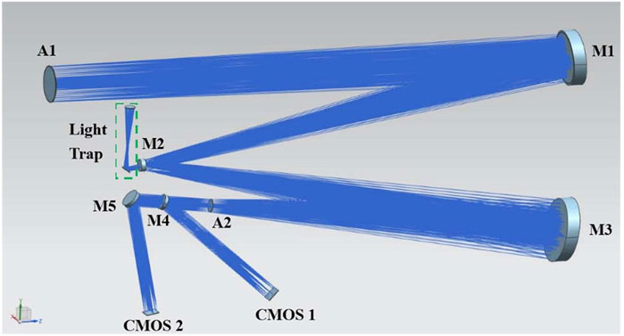
FIGURE 1. Schematic optical layout of SCI.

The sunlight illuminates the off-axis parabolic primary mirror (M1) through the entrance aperture (A1). M1 images the solar disk and the corona on a convex secondary mirror (M2), which has a cone-shaped hole to ensure the solar disk light passes through and enters the light trap behind M2. Then, the coronal light remains and is reflected from M2 to an off-axis third mirror (M3). A Lyot stop (A2) is placed in the conjugate plane of A1 imaged by M1, M2, and M3 to block the light diffracted from the edge of A1. A beam splitter (M4) composed of a multilayer film is used to separate the Lyman-alpha corona and the white-light corona to CMOS 1 and CMOS 2 [10].

3 Stray-Light Suppression of SCI

The brightness of the corona is extremely weak compared to that of the solar disk, as shown in Figure 2 [11]. In order to observe the corona from 1.1 to 2.5 R_⊙, the stray-light suppression level must be as low as 10⁻⁴ to 10⁻⁶ B_⊙ in Lyman-alpha wavebands and 10⁻⁶ to 10⁻⁸ B_⊙ in white-light wavebands. Therefore, stray-light suppression becomes the most important issue for SCI. Three main stray-light sources need to be suppressed, including the direct stray-light from the solar disk, the diffracted stray-light from the edge of A1 that is illuminated by the Sun, and the scattered stray-light from M1. For an internally occulted reflecting coronagraph, the scattered stray-light from the primary mirror determines the stray-light suppression level [12–15]. Owing to the extremely high requirements for stray-light suppression in the white-light wavebands, detailed analysis of the scattered stray-light in the white-light wavebands is required.

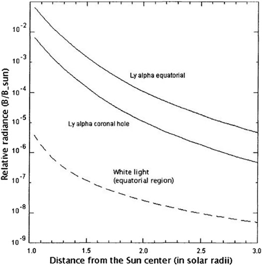
FIGURE 2. Brightness of the corona compared to the solar disk in Lyman-alpha and white-light wavebands.

3.1 Direct Stray-Light From the Solar Disk

Because of no external occulter in front of M1 to block the solar disk light, the light will directly enter SCI and become the first source of stray-light. In order to eliminate the direct light from the solar disk, M2 is designed with a cone-shaped hole at the center as the internal occulter, which is located at the focal position of M1, to ensure that the solar disk light passes through and enters the light trap behind it. The taper of the cone-shaped hole is greater than the divergence angle of the light after M2 converges so that the direct light from the solar disk will not be scattered inside the cone-shaped hole. In order to reduce the concentration of solar energy in the light trap, a spherical collimating mirror is designed behind M2, and then the solar disk light is reflected to the plane mirror and finally absorbed by Acktar Absorbent Panels. The solar disk light will not return to the coronal imaging path to become stray-light. The ray-tracing process is shown in Figure 3. The design of the cone-shaped hole inside M2 and light trap ensures the elimination of direct stray-light from the solar disk.

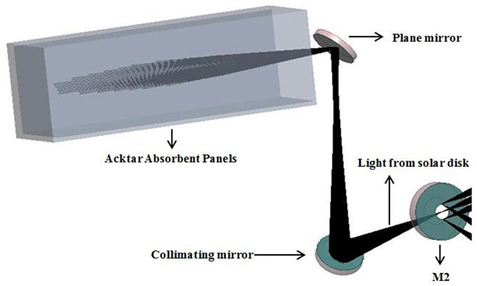
FIGURE 3. Ray-tracing diagram of direct stray-light from the solar disk.

3.2 Diffracted Stray-Light From the Edge of the Entrance Pupil A1

Since the entrance pupil A1 is directly exposed to strong sunlight, strong diffracted stray-light will be generated that need to be suppressed when the sunlight hits the edge of A1. The Lyot stop A2 is designed at the conjugate position of A1 imaged by M1, M2, and M3, to block the diffracted stray-light. The diffracted stray-light is displayed in Figure 4. By establishing a coherent light source with a wavelength of 700.0 nm at the position of A1, the distribution of the diffracted stray-light is simulated at its conjugate position, as shown in Figure 4A. The diffracted image of A1 is distributed in the range of its conjugate surface from 21.0 to 22.4 mm (shown in Figures 4B,C). The design of the Lyot stop A2 with the diameter of 21.0 mm can effectively prevent the diffracted stray-light from reaching the focal plane. The diffracted stray-light effect of 121.6 nm is similar to that of 700.0 nm, and the same size of A2 can block the diffracted stray-light of 121.6 nm, which is not repeated here.

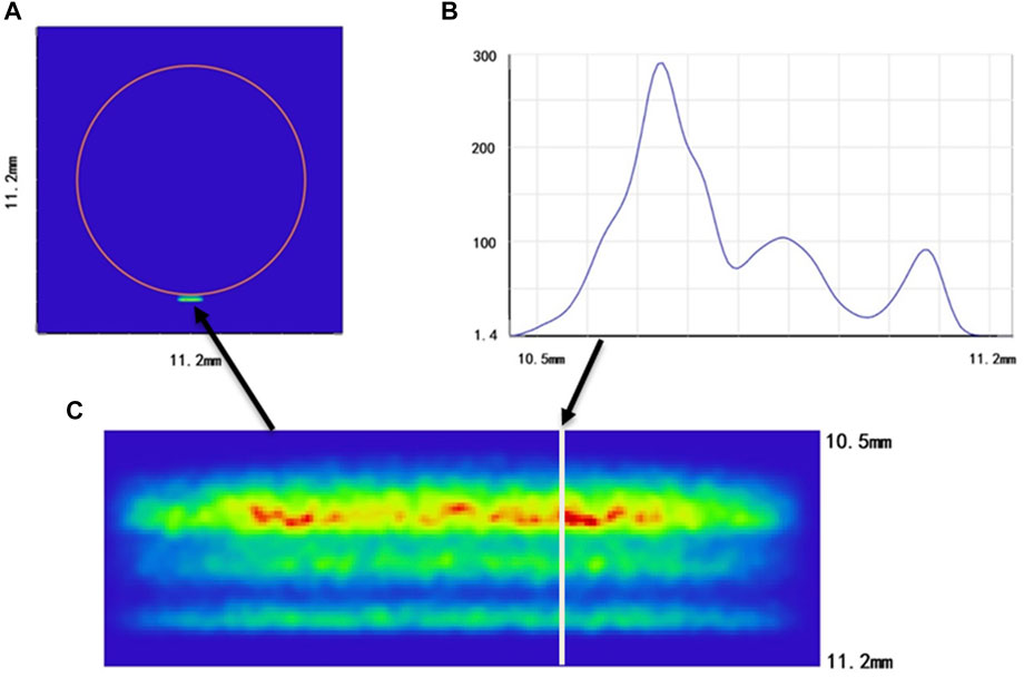
FIGURE 4. Simulation results of diffracted stray-light at 700.0 nm. (A) Diffracted stray-light image at the Lyot stop A2 position. (B) Relative intensity distribution curve of diffracted stray-light from a radius of 10.5–11.2 mm. (C) Partial enlarged view of a diffracted stray-light image.

3.3 Scattered Stray-Light From the Primary Mirror M1

For an internally occulted reflecting coronagraph such as SCI, the solar disk light will directly illuminate the surface of the primary mirror M1, and strongly scattered stray-light is generated, which contributes the majority of the stray-light. It has been demonstrated that the stray-light level of the LASCO C1 coronagraph—an internally occulted coronagraph similar to SCI—is determined by the surface quality of the primary mirror [16]. Therefore, in order to achieve the high stray-light suppression level for SCI, excellent surface quality of the primary mirror is also required. The scattered stray-light resulting from the surface quality of the primary mirror needs to be analyzed and suppressed with emphasis, including the contribution of surface errors, cosmetic defects, and particulate contamination to the stray-light for SCI.

3.3.1 Scattered Stray-Light From Surface Errors of M1

In order to accurately evaluate the influence of the surface errors on the scattering, it is necessary to measure the surface errors in all relevant spatial frequencies. The power spectral density (PSD) of surface errors as a function of the spatial frequencies is accepted as an all-inclusive way to characterize optical surfaces, which can quantitatively describe the distribution of super-polished surface topography in spatial frequency ranges, and provides abundant data for the analysis of surface errors. The PSD [17] curve over the entire spatial frequency ranges can be obtained by Fourier transform of the surface profile errors as follows:

Here, L is the sampling length that can represent its geometric characteristics. It is the diameter of the mirror if sampling using an interferometer, and it is the field-of-view corresponding to different objective magnifications if sampling using a white-light optical profiler. z (x) is the surface profile error function, and “x” is the 1D coordinates of the sample along the surface. f is the spatial frequency. Equation (1) can be used to evaluate whether the surface errors of M1 meet the stray-light requirement for SCI. It is of great guidance to the surface polishing improvement.

According to the Harvey–Shack scattering theory, surface errors in different spatial frequency ranges have different effects on imaging quality [18–20]. Low-spatial frequency surface errors produce conventional aberrations, which affect the convergence of the Sun at the position of M2 and result in the stray-light of the inner FOV for SCI; mid-spatial frequency surface errors produce small-angle scattering, which affects the stray-light level of the inner FOV for SCI; and high-spatial frequency surface errors produce large-angle scattering, which affects the stray-light level of the outer FOV for SCI. Therefore, it is necessary to specify and measure the surface errors of M1 over the entire spatial frequency ranges to ensure that M1 meets the requirement, thereby suppressing the stray-light over the full FOV for SCI.

To specify the contribution of surface errors of M1 to the stray-light level, the Harvey–Shack ABg bidirectional scattering distribution function (BSDF) model is applied to characterize the surface errors of M1. This model is suitable for the scattering mainly caused by roughness, and the RMS roughness is much less than the wavelength. The BSDF function of an optical surface with an RMS roughness of “σ” [21, 22] is expressed in Eq. (2):

Here, $A=\raisebox{1ex}{$\pi $}\!\left/ \!\raisebox{-1ex}{$2$}\right.\cdot \raisebox{1ex}{$\mathit{\Delta }{n}^2{\sigma }^2$}\!\left/ \!\raisebox{-1ex}{${\mathit{\lambda }}^2$}\right.$, $B={\left(\raisebox{1ex}{$\mathit{\lambda }$}\!\left/ \!\raisebox{-1ex}{$2\pi l$}\right.\right)}^2$, and g is the logarithmic slope of the tail of BSDF. It is a dimensionless constant and is usually taken as 2, △n is the change in the refractive index (△n = 2 for mirrors), and λ is the wavelength. l is the auto-correlation length related to the scattering properties. When the RMS roughness of M1 is 0.3 nm and the wavelength is 700.0 nm, then A = 1.15 × 10⁻⁶ andB = 1.24 × 10⁻⁶; the BSDF resulting from surface errors of M1 is shown in Figure 5A. A simulated solar disk source with a divergence angle of 32′ is established in non-sequential ray-tracing software to illuminate the SCI, and the stray-light distribution at the focal plane is simulated as shown in Figure 5B. Under this condition, the irradiance of the stray-light and the solar disk source at the focal plane can be obtained, and the ratio of the two represents the stray-light suppression level. Simulation results show that the stray-light suppression level can be as low as 10⁻⁷ B_⊙ at 1.1 R_⊙ and 10⁻⁸ B_⊙ at 2.5 R_⊙.

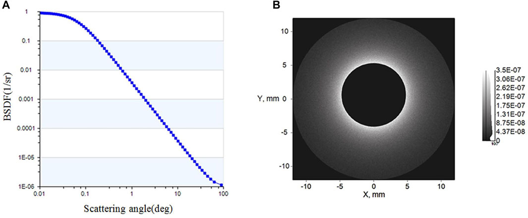
FIGURE 5. Scattered stray-light simulation results from surface errors of M1 at 700 nm. (A) BSDF curve as a function of the scattering angle for M1 due to a surface roughness of 0.3 nm at 700 nm. (B) Stray-light distribution at the focal plane (CMOS2).

When the wavelength is 121.6 nm, then A = 3.82 × 10⁻⁵ andB = 3.75 × 10⁻⁸; the BSDF resulting from the surface errors of M1 is shown in Figure 6A, and the stray-light distribution at the focal plane is shown in Figure 6B. The stray-light suppression level can be as low as 10⁻⁵ B_⊙ at 1.1 R_⊙ and 10⁻⁶ B_⊙ at 2.5 R_⊙.

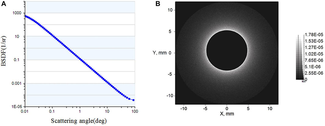
FIGURE 6. Scattered stray-light simulation results from surface errors of M1 at 121.6 nm. (A) BSDF curve as a function of the scattering angle for M1 due to a surface roughness of 0.3 nm at 121.6 nm. (B) Stray-light distribution at the focal plane (CMOS1).

After specifying surface errors of M1, different metrology instruments (laser interferometer for low-spatial frequency and white-light optical profiler for mid-spatial and high-spatial frequencies) are required to measure them. The spatial frequency range of different metrology instruments for measuring surface errors is determined by the sampling length L and the resolution of CMOS [23]. The minimum spatial frequency that can be measured is 1/L, where L is the FOV corresponding to different objective magnifications for the white-light optical profiler or the measurable aperture diameter for the laser interferometer. The maximum spatial frequency that can be measured is 1/(2d), which is the Nyquist cut-off frequency, where d is the sampling interval corresponding to the pixel size of CMOS [24, 25].

Since surface scatter phenomenon is a diffraction process, according to the grating equation (26), components with a spatial frequency greater than 1/λ will produce a small amount of optical scattering for SCI, which can be ignored. Therefore, the upper limit of the spatial frequency of the PSD curve is 1/λ, and the lower limit of the frequency is 1/D, where D is the aperture diameter of M1. According to the metrology data for different measuring instruments [27] in their specified spatial frequencies, the PSD [28] curve over the entire spatial frequencies is shown in Figure 7, which is obtained by Eq. 1. While measuring the surface errors, random errors such as mechanical vibration and electronic noise are removed by multiple phase averaging, and the system error is removed by subtracting the surface errors of the standard sample. The metrology data after removing random errors and system errors are under the PSD limit line of the polishing requirement; otherwise, another polishing and testing cycle is necessary.

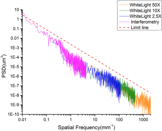
FIGURE 7. Composite surface PSD function of M1 determined from different metrology instruments.

3.3.2 Scattered Stray-Light From Cosmetic Defects of M1

Scratches and digs on the optical surface are cosmetic defects, which will generate unnecessary light scattering and contribute to stray-light for SCI. In order to quantify the stray-light level from cosmetic defects, a dark-field microscope is used to measure the number and size of scratches and digs on M1. The sub-field testing results are shown in Figure 8, in which mark 1 is a scratch, marks 2–5 are digs, and 6–9 are dust.

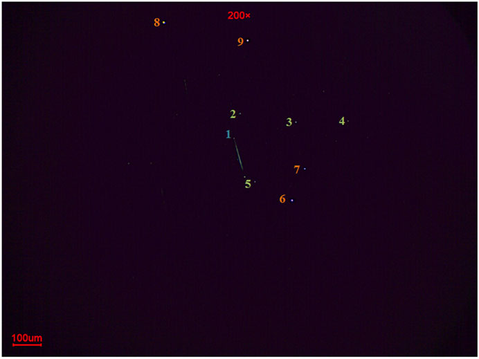
FIGURE 8. Sub-field testing results from cosmetic defects using a dark-field microscope.

According to the Gary L. Peterson’s cosmetic defects scattering theory, stray-light due to scratches or digs includes geometric refraction inside the scratches or digs and diffraction of light that passes around scratches or digs can be quantitatively analyzed by BSDF.

BSDF from scratches [29] is given by the expression:

Here, $N_s=\frac{1}{\mathit{\pi }lD}$, $l_s={\left(\frac{1}{2{\mathit{\pi }}^2}\right)}^{\raisebox{1ex}{$2$}\!\left/ \!\raisebox{-1ex}{$3$}\right.}\frac{\mathit{\lambda }}{{\left(w^{2}l\right)}^{\raisebox{1ex}{$1$}\!\left/ \!\raisebox{-1ex}{$3$}\right.}}$, N_s is the density of the scratches (number of scratches per unit area), D is the diameter of the optical element, w and l are their typical width and length from microscopy, respectively, θ is the scattering angle with respect to the surface normal of the optical component, and l_s is the roll-off angle of the BSDF curve. We note that the factor l in the numerator of Eq. (3) will cancel with the factor of l in N_s, so the width has a dominant effect on the BSDF from scratches. According to the statistical testing results of scratches for M1 over the full FOV, the typical width w is less than 0.002 mm.

The Harvey–Shack scattering model based on the scalar diffraction theory can predict the scattering distribution of a super-polished optical surface, which is given by the expression:

Here, b₀ is the intercept of the BSDF at the specular angle, θ is the scattering angle, and L is the shoulder of the BSDF curve and equals the sine of the shoulder angle. According to the calculation result of BSDF from scratches, a fitting Harvey–Shack scattering model is established with b₀ = 3 × 10⁻², L = 2 × 10⁻³, and s = -2. The fitting BSDF curve is shown in Figure 9A, and the simulated stray-light distribution resulting from scratches is shown in Figure 9B.

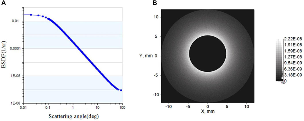
FIGURE 9. Scattered stray-light simulation results from scratches of M1 at 700 nm. (A) BSDF curve as a function of the scattering angle. (B) Stray-light distribution at the focal plane.

BSDF from digs is given by the expression:

Here, $N_d=\raisebox{1ex}{$1$}\!\left/ \!\raisebox{-1ex}{$5\mathit{\pi }D$}\right.$, $l_d={\left(\frac{4}{{\mathit{\pi }}^4}\right)}^{\raisebox{1ex}{$1$}\!\left/ \!\raisebox{-1ex}{$3$}\right.}\frac{\mathit{\lambda }}{d}$, N_d is the density of the digs (number of digs per unit area), d is the diameter of the dig from microscopy, θ is the scattering angle, l_d is the roll-off angle, and D is the diameter of the optical element. Combined with the statistical testing result of digs for M1 over the full FOV, the diameter of the dig d is less than 0.01 mm. According to the calculation result of BSDF from digs, a fitting Harvey–Shack scattering model is established with b₀ = 1 × 10⁻⁵, L = 2 × 10⁻², and s = −2. The fitting BSDF curve is shown in Figure 10A, and the simulated stray-light distribution resulting from digs at 700.0 nm is shown in Figure 10B.

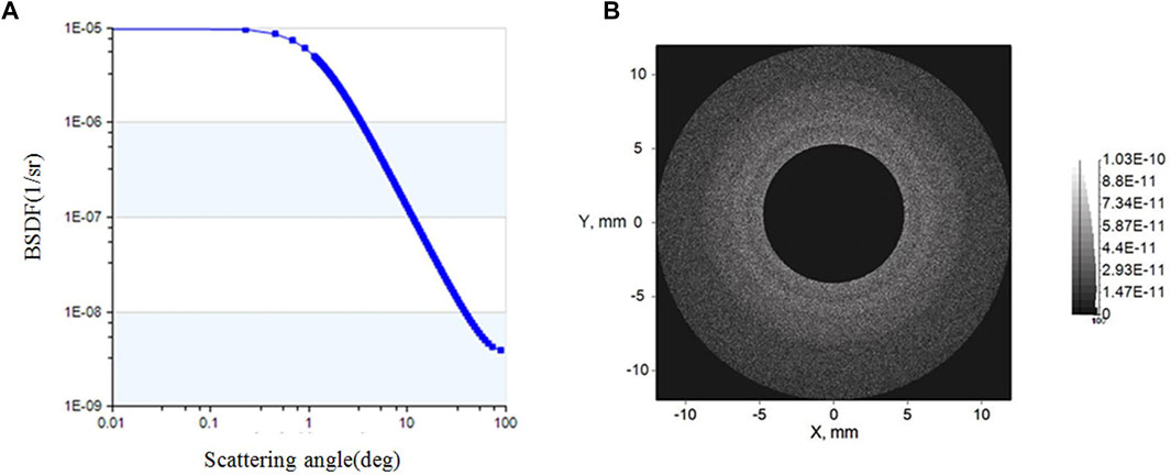
FIGURE 10. Scattered stray-light simulation results from digs of M1 at 700.0 nm. (A) BSDF curve as a function of the scattering angle. (B) Stray-light distribution at the focal plane.

3.3.3 Scattered Stray-Light From Particulate Contamination of M1

The surface BSDF scattering resulting from particulate contamination is a function of the particle density function f(D) [30]. According to the Mie scattering theory, BSDF can be estimated when the MIL-STD-1264B Cleanliness Level (CL) is used to describe f(D). Spyak and Wolfe’s work shows that particulate contamination scattering is also shift invariant, and the Harvey–Shack model can be used to predict particle scattering in accordance with Spyak and Wolfe’s BSDF curve. For particulate contamination scattering [31], the parameter b₀ in Eq. (4) can be taken by the total integrated scattering (TIS) [32] corresponding to the cleanliness level of M1 as follows:

According to the statistical testing results of dust for M1 over the full FOV, the cleanliness level for M1 is better than class 100, and the fitting parameters are inserted into the Harvey–Shack scattering model with L = 2 × 10⁻², TIS = 1.3 × 10⁻⁵, b₀ = 2 × 10⁻³, and s = −2.2. The BSDF curve for cleanliness level 100 at 700.0 nm is shown in Figure 11A, and the simulated stray-light distribution resulting from particulate contamination is shown in Figure 11B.

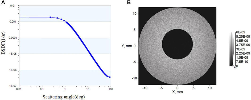
FIGURE 11. Scattered stray-light simulation results from particulate contamination with CL100 at 700.0 nm. (A) BSDF curve as a function of the scattering angle. (B) Stray-light distribution at the focal plane.

According to the aforementioned BSDF Eqs. 2–5, combined with the testing results of the white-light optical profiler and the dark-field microscope for M1, the BSDF scattering curves resulting from roughness (red line), scratches (violet line), digs (green line), and particulate contamination with cleanliness level 100 (blue line) at 700.0 nm are shown in Figure 12. Their contributions to the stray-light level for SCI are shown in Table 1. After using the aforementioned testing results for stray-light simulation, the overall stray-light level for SCI can be suppressed to 10⁻⁸ B_⊙ at 700.0 nm.

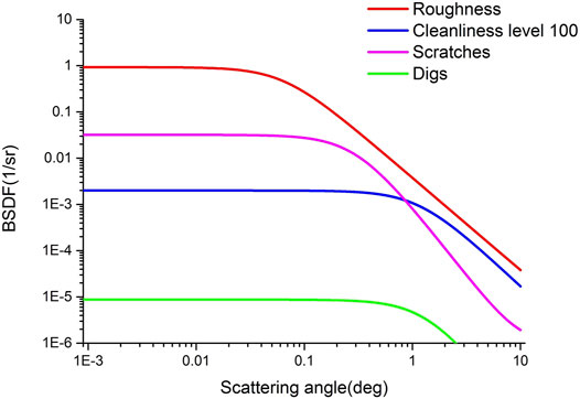
FIGURE 12. BSDF curves as a function of the scattering angle for SCI M1 at 700.0 nm.

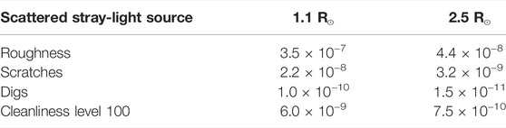
TABLE 1. Summary of scattered stray-light level contributions at 700.0 nm.

4 Stray-Light Measurement for SCI

After analyzing the various factors that affect the stray-light suppression level of SCI, it is necessary to measure it in our laboratory. The stray-light measurement device includes a solar radiation simulator and a cooled CMOS camera as shown in Figure 13. A xenon lamp illuminates a diffuser and aperture mounted at the focal plane of the collimator to form a beam of simulated solar disk light [33]. The diameter of the aperture can be determined by $D=f\cdot \tan \Omega$, where f is the focal length of the collimator and Ω is the divergence angle of the simulated solar disk light and equals to 32′.

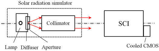
FIGURE 13. Schematic diagram of the stray-light measurement device.

While measuring stray-light, the optical axis of the solar radiation simulator is aligned with SCI, the solar disk light passes through M2 and enters the light trap of SCI, and the cooled CMOS camera only receives the stray-light image, as shown in Figure 14A. Then, the SCI is rotated and an attenuator is added so that the solar disk light illuminates the imaging area of M2, and the solar disk is imaged on the camera, as shown in Figure 14B. The full well of the camera is 51400 e, the readout noise is 1.5 e, the frame rate is set to 0.02, and 16-bit images are obtained. The stray-light suppression level of SCI is represented by the brightness ratio of the stray-light to the solar disk as B_stray/B_sun. The measurement should be carried out in an ultra-clean laboratory to reduce the impact of ambient stray-light caused by the scattering of particles in the air. In addition, the solar simulator should be installed inside a black shading box and far enough from SCI to ensure that stray-light from the solar simulator cannot enter SCI.

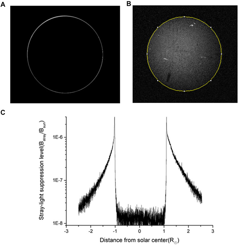
FIGURE 14. (A) Stray-light image. (B) Solar disk image. (C) Stray-light suppression level as a function of the distance from the solar center.

The measurement results show that the stray-light can be suppressed to the order of 10⁻⁸ B_⊙ at 700.0 nm, which is consistent with the simulation results combined with the testing surface roughness, cosmetic defects, and particulate contamination of the primary mirror.

5 Discussion

In this study, the main sources of stray-light were analyzed and suppressed in detail, including the scattered stray-light from the primary mirror, the direct stray-light from the solar disk, and the diffracted stray-light from the edge of the entrance pupil. The surface errors, cosmetic defects, and particulate contamination of the primary mirror were tested in the laboratory. Based on the testing results, the corresponding scattering model was established for simulation, and the stray-light suppression level was verified via the laboratory stray-light measurement, and the influence of surface quality characteristics on the stray-light level for SCI was demonstrated. This modeling and simulation method based on the individual mirror laboratory testing is suitable for stray-light analysis and suppression of all coronagraphs.

Data Availability Statement

The datasets presented in this article are not readily available because simulation and experimental data are obtained through repeated theoretical and practical research. Requests to access the datasets should be directed to GZ, zhangguang0920@163.com.

Author Contributions

GZ contributed to the idea, modeling, and simulation of the stray-light suppression method. YW contributed to the design of the Solar Corona Imager and partial simulation. LH contributed to the measurement method. XW and SR contributed to the testing of the mirror. YX and FL performed the image data processing. BC modified the writing.

Funding

This work was partially supported by the Strategic Pioneer Program on Space Science of the Chinese Academy of Sciences (Grant No. XDA15320103), the National Natural Science Foundation of China (Grant No. 11427803), and the Joint Research Fund in Astronomy (Grant No. U2031122) under cooperative agreement between the National Natural Science Foundation of China and Chinese Academy of Sciences.

Conflict of Interest

The authors declare that the research was conducted in the absence of any commercial or financial relationships that could be construed as a potential conflict of interest.

Publisher’s Note

All claims expressed in this article are solely those of the authors and do not necessarily represent those of their affiliated organizations, or those of the publisher, the editors, and the reviewers. Any product that may be evaluated in this article, or claim that may be made by its manufacturer, is not guaranteed or endorsed by the publisher.

References

1. Koomen MJ, Detwiler CR, Brueckner GE, Cooper HW, Tousey R. White Light Coronagraph in OSO-7. Appl. Opt. (1975) 14:743–51. doi:10.1364/AO.14.000743
2. Domingo V, Fleck B, Poland AI. The SOHO Mission: An Overview. Sol Phys (1995) 162:1–37. doi:10.1007/BF00733425
3. Frazin RA, Vásquez AM, Thompson WT, Hewett RJ, Lamy P, Llebaria A, et al. Intercomparison of the LASCO-C2, SECCHI-COR1, SECCHI-COR2, and Mk4 Coronagraphs. Sol Phys (2012) 280:273–93. doi:10.1007/s11207-012-0028-3
4. Kaiser ML, Kucera TA, Davila JM, St. Cyr OC, Guhathakurta M, Christian E. The STEREO Mission: An Introduction. Space Sci Rev (2008) 136:5–16. doi:10.1007/s11214-007-9277-0
5. Fineschi S, Antonucci E, Naletto G, Romoli M, Spadaro D, Nicolini G, et al. Metis: a Novel Coronagraph Design for the Solar Orbiter Mission. Proc. SPIE (2012) 8443:844384433H. doi:10.1117/12.927229
6. Venkata SN, Prasad BR, Nalla RK, Singh J. Scatter Studies for Visible Emission Line Coronagraph on Board ADITYA-L1 Mission. J. Astron. Telesc. Instrum. Syst (2017) 3:014002. doi:10.1117/1.JATIS.3.1.014002
7. Chen B, Li H, Song K-F, Guo Q-F, Zhang P-J, He L-P, et al. The Lyman-alpha Solar Telescope (LST) for the ASO-S Mission - II. Design of LST. Res. Astron. Astrophys. (2019) 19:159. doi:10.1088/1674-4527/19/11/159
8. Gong Q, Socker D. Theoretical Study of the Occulted Solar Coronagraph. Proc. SPIE (2004) 5526:208–19. doi:10.1117/12.549275
9. Wang YQ, Zhang G, He LP, Guo QF, Zhang HJ, Wang HF, et al. Solar Coronagraph Imager Based on Internal Occulting in Lyman-alpha and Visible Bands. Opt Precis Eng (2019) 28:303–14.
10. Wang X, Chen B, Huo T, Zhou H. Design of Second-Order 121.6-nm Narrowband Minus Filters Using Asymmetrically Apodized Thickness Modulation. Appl. Phys. B (2018) 124:1–6. doi:10.1007/s00340-018-7010-1
11. Vives S, Lamy PL, Vial J-C. Optical Design of the Lyman Alpha Coronagraph for the LYOT Microsatellite. Proc. SPIE (2004) 5171:298–306. doi:10.1117/12.506390
12. Fineschi S, Romoli M, Hoover RB, Baker PC, Zukic M, Kim J, et al. Stray Light Analysis of a Reflecting UV Coronagraph/Polarimeter with Multilayer Optics. Proc. SPIE (1994) 78–92. doi:10.1117/12.168591
13. Romoli M, Weiser H, Gardner LD, Kohl JL. Stray-Light Suppression in a Reflecting White-Light Coronagraph. Appl. Opt. (1993) 32:3559–69. doi:10.1364/AO.32.003559
14. Newkirk G, Bohlin D. Reduction of Scattered Light in the Coronagraph. Appl. Opt. (1963) 2:131–40. doi:10.1364/AO.2.000131
15. Landini F, Romoli M, Fineschi S, Antonucci E. Stray-light Analysis for the SCORE Coronagraphs of HERSCHEL. Appl. Opt. (2006) 45:6657–67. doi:10.1364/AO.45.006657
16. Brueckner GE, Howard RA, Koomen MJ, Korendyke CM, Michels DJ, Moses JD, et al. The Large Angle Spectroscopic Coronagraph (LASCO). Sol Phys (1995) 162:357–402. doi:10.1007/978-94-009-0191-9_1010.1007/bf00733434
17. Youngworth RN, Gallagher BB, Stamper BL. An Overview of Power Spectral Density (PSD) Calculations. Proc.of SPIE (2005) 586958690U. doi:10.1117/12.618478
18. Youngworth RN, Stone BD. Simple Estimates for the Effects of Mid-spatial-frequency Surface Errors on Image Quality. Appl. Opt. (2000) 39:2198–209. doi:10.1364/AO.39.002198
19. Stover JC, Harvey JE. Limitations of Rayleigh Rice Perturbation Theory for Describing Surface Scatter. Proc. SPIE (2007) 667266720B. doi:10.1117/12.739133
20. Harvey JE. Integrating Optical Fabrication and Metrology into the Optical Design Process. Appl. Opt. (2015) 54:2224–33. doi:10.1364/AO.54.002224
21. Harvey JE, Choi N, Schroeder S, Duparré A. Total Integrated Scatter from Surfaces with Arbitrary Roughness, Correlation Widths, and Incident Angles. Opt. Eng (2012) 51:013402. doi:10.1117/1.OE.51.1.013402
22. Choi N, Harvey JE. Numerical Validation of the Generalized Harvey-Shack Surface Scatter Theory. Opt. Eng (2013) 52:115103. doi:10.1117/1.OE.52.11.115103
23. Grochocki F, Fleming J. Stray Light Testing of the OLI Telescope. Proc. SPIE (2010) 7794:779477940W. doi:10.1117/12.862225
24. Lang Z, Qiao S, Ma Y. Acoustic Microresonator Based In-Plane Quartz-Enhanced Photoacoustic Spectroscopy Sensor with a Line Interaction Mode. Opt. Lett. (2022) 47:1295–8. doi:10.1364/OL.452085
25. Liu X, Ma Y. Sensitive Carbon Monoxide Detection Based on Light-Induced Thermoelastic Spectroscopy with a Fiber-Coupled Multipass Cell [Invited]. 中国光学快报 (2022) 20:031201. doi:10.3788/COL202220.031201
26. Harvey JE, Thompson AK. Scattering Effects from Residual Optical Fabrication Errors. Proc. SPIE (1995) 2576:155–74. doi:10.1117/12.215588
27. Church EL, Takacs PZ. Instrumental Effects in Surface Finish Measurement. Proc. SPIE (1989) 1009:46–55. doi:10.1117/12.949154
28. Dittman MG. K-correlation Power Spectral Density and Surface Scatter Model. Proc.of SPIE (2006) 6291:629162910R. doi:10.1117/12.678320
29. Peterson GL. A BRDF Model for Scratches and Digs. Proc.of SPIE (2012) 8495:849584950G. doi:10.1117/12.930860
30. Spyak PR, Wolfe WL. Scatter from particulate-contaminated mirrors. part 3: theory and experiment for dust and lambda=10.6 um. Opt. Eng. (1992) 31:1764–74. doi:10.1117/12.58710
31. Spyak PR, Wolfe WL. Scatter from Particulate-Contaminated Mirrors. Part 4: Properties of Scatter from Dust for Visible to Far-Infrared Wavelengths. Opt. Eng. (1992) 31:1775–84. doi:10.1117/12.58711
32. Dittman MG. Contamination Scatter Functions for Stray-Light Analysis. Proc.of SPIE (2002) 4774:99–110. doi:10.1117/12.481666
Keywords: solar corona imager, internally occulted reflecting coronagraph, stray-light, surface quality, scattering
Citation: Zhang G, Wang Y, He L, Wang X, Ren S, Xuan Y, Liu F and Chen B (2022) Stray-Light Suppression of the Internally Occulted Reflecting Solar Corona Imager. Front. Phys. 10:890197. doi: 10.3389/fphy.2022.890197
Received: 05 March 2022; Accepted: 13 April 2022;
Published: 09 June 2022.
Edited by:
Yufei Ma, Harbin Institute of Technology, ChinaReviewed by:
Sanjay Gosain, National Solar Observatory, United StatesDebi Prasad Choudhary, California State University, Northridge, United States
Ziyang Chen, Huaqiao University, China
Copyright © 2022 Zhang, Wang, He, Wang, Ren, Xuan, Liu and Chen. This is an open-access article distributed under the terms of the Creative Commons Attribution License (CC BY). The use, distribution or reproduction in other forums is permitted, provided the original author(s) and the copyright owner(s) are credited and that the original publication in this journal is cited, in accordance with accepted academic practice. No use, distribution or reproduction is permitted which does not comply with these terms.
*Correspondence: Bo Chen, chenb@ciomp.ac.cn