Predicting Coherent Turbulent Structures via Deep Learning
 D. Schmekel1
  F. Alcántara-Ávila
 R. Vinuesa
- 1FLOW, Engineering Mechanics, KTH Royal Institute of Technology, Stockholm, Sweden
- 2Instituto de Matemática Pura y Aplicada, Universitat Politècnica de València, València, Spain
Turbulent flow is widespread in many applications, such as airplane wings or turbine blades. Such flow is highly chaotic and impossible to predict far into the future. Some regions exhibit a coherent physical behavior in turbulent flow, satisfying specific properties; these regions are denoted as coherent structures. This work considers structures connected with the Reynolds stresses, which are essential quantities for modeling and understanding turbulent flows. Deep-learning techniques have recently had promising results for modeling turbulence, and here we investigate their capabilities for modeling coherent structures. We use data from a direct numerical simulation (DNS) of a turbulent channel flow to train a convolutional neural network (CNN) and predict the number and volume of the coherent structures in the channel over time. Overall, the performance of the CNN model is very good, with a satisfactory agreement between the predicted geometrical properties of the structures and those of the reference DNS data.
Introduction
Fluid flow is vital for a large variety of applications such as aircraft, heat pumps, lubrication, etc. [1]. Typically, for many applications, the flow is in a turbulent regime [1]. Such flow is characterized by being chaotic and highly non-linear, with large mixing amounts. Consequently, turbulent flow is a challenge to modellers [2]. It has been estimated that turbulence is responsible for up to 5% of the total CO2 generated by humanity every year [3]. Even small gains in understanding turbulence can be very impactful. Fluid flow, including turbulent flow, is described by the Navier–Stokes equations, which are generally impossible to solve analytically. They can be solved numerically, but this has traditionally been prohibitively computationally expensive—only elementary geometries have been simulated [4,5]. In recent years, it has become possible to perform high-fidelity simulations of complex geometries [6–9].
One of the earlier studies on the structure of turbulence was carried out by Kline et al. [10]. Kline et al. also investigated the statistical properties of turbulence and found that most of the turbulence production takes place near the walls (at least at low Reynolds numbers). They observed specific regions in the flow, called coherent turbulent structures, which we will denote as structures. One essential type of coherent structure is strongly related to Reynolds stresses [11]. Typically, these Reynolds-stress structures may occupy around 4% of the volume but can be responsible for around 30% of the Reynolds stresses. The structures are also important for the transfer of several properties such as mass, heat, and momentum [12]. Many models created for studying turbulence are built upon these structures [13]. Traditionally, the focus of structures has been on hairpins, U-shaped structures formed near walls going to the outer region[14]. Hairpins were the basic building block in several models [15–17], which formed hairpin clusters [14]. Objections to these models have arisen since they have had problems at higher Reynolds numbers [18]. Instead, momentum-transfer models have been created, focusing on strong Reynolds-stress and momentum-transfer events. Some data supports these types of models for modeling momentum transfer in the logarithmic layer [13].
In this study we will use deep neural networks (DNNs), which are black-box methods [19,20] and are universal function approximators. They can approximate any sufficiently smooth function arbitrarily well. In the DNN framework, it is assumed that the phenomena under study can be described by some predetermined parameterizable function f(x; Θ), where Θ are the parameters. The values of Θ that best approximate the data are obtained by means of algorithms such as stochastic gradient descent and the back-propagation [21]. DNNs have been used successfully for modelling the temporal dynamics of turbulence [22,23], for non-intrusive sensing [24,25], for identifying patterns in complex flows [26] and for modelling the Reynolds stresses [27]. Two overviews of the current applications of DNNs in fluid mechanics can be found in [2,28]. Here we investigate the possibilities to predict the temporal evolution of coherent turbulent structures with machine-learning techniques. To this end, we create a DNN-based mode and assess the quality of its predictions, in terms of the number of structures, the total volume of the structures, and the volume of the largest structure. The goal is to develop a model capable of estimating plausible future scenarios of the flow, focusing on the characteristics of the turbulent structures. We also expect this model to exhibit appropriate generalization properties [29].
The article is structured as follows: in §2 we discuss the data collection and the network design; in §3 we present our results; and finally conclusions and discussions are presented in §4.
Methods
Numerical Setup
We study wall-bounded turbulent structures in a turbulent channel flow, consisting of two infinitely large planes parallel to the x (streamwise) and z (spanwise) directions. The distance between the planes is 2h. Figure 1 shows an illustration of problem. A pressure gradient in the streamwise direction drives the flow, which has a friction Reynolds number Reτ = 125. The friction Reynolds number, defined as Reτ = uτh/ν, is the main control parameter in wall bounded turbulence. Here
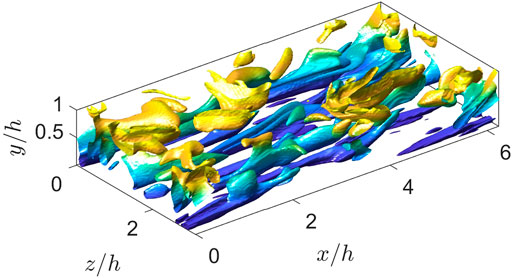
FIGURE 1. Reyhnolds-stress structures at the bottom half of the channel. The structures are coloured by wall-normal distance. The flow moves from the left to the right of the figure.
This simulation has been performed in a computational box of sizes Lx = 2πh, Ly = 2h and Lz = πh. This box is large enough to accurately describe the statistics of the flow [30,31]. The streamwise, wall-normal, and spanwise velocity components are U, V and W or, using index notation, Ui. Statistically-averaged quantities in time, x and z are denoted by an overbar,
where repeated subscripts indicate sumation over 1, 2, 3 and the pressure term includes the density. These equations have been solved using the LISO code [4], similar to the one described by Lluesma-Rodríguez et al. [32]. This code has successfully been employed to run some of the largest simulations of wall-bounded turbulent flows [4,33–37]. Briefly, the code uses the same strategy as that described by Kim et al. [38], but using a seven-point compact-finite-difference scheme in the y direction with fourth-order consistency and extended spectral-like resolution [39]. The temporal discretization is a third-order semi-implicit Runge–Kutta scheme [40]. The wall-normal grid spacing is adjusted to keep the resolution to Δy = 1.5η, i.e., approximately constant in terms of the local isotropic Kolmogorov scale
As a consequence of the self-sustaining mechanism, coherent structures in the form of counter-rotating rolls are triggered by pairs of ejections and sweeps extending beyond the buffer layer in a well-organised process called bursting. The ejections carry low streamwise velocity upwards from the wall (u < 0, v > 0), while the sweeps carry high streamwise velocity downwards to the wall (u > 0, v < 0). Based on a Reynolds stress quadrant classification, ejections and sweeps are Q2 and Q4 events, respectively. Lozano-Duran et al. [13] and Jiménez [18] reported the relation between counter-rotating rolls, streamwise streaks and Q2-Q4 pairs in turbulent Poiseuille flow by observing averaged flow fields conditioned to the presence of a wall-attached Q2-Q4 pair. A wall-attached event is an intense Reynolds stress structure (i.e. uv-structure) that approaches a wall below y+ < 20. The reasoning for this definition is explained later. For a time-resolved view of the bursting process in turbulent Poiseuille channel at Reτ ≈ 4,200, the interested reader is referred to [30]. Gandía Barberá et al. [41] performed this process again for Couette flows in presence of stratification.
In order to study the underlying physics of the flow, the coherent structures responsible for the transport of momentum are analysed. Jiménez [18] discussed that the intensity of a given parameter is considered as an indicator of coherence, among other characteristics. However, the selection of a threshold is only feasible if the parameter is intermittent enough to separate between high- and low-intensity regions. After analysing the intermittency of different parameters, it is found that quadratic parameters, specially the Reynolds stress, are more appropriate to describe intense coherent structures.
We are interested in using a DNN to predict how these structures evolve. Running the code we obtain a three-dimensional (3D) instantaneous flow fields (snapshots) sequence. Since the flow in the channel is statistically symmetric, we will only use the lower half of the channel for faster calculations. The final snapshots have 96 × 76 × 96 grid points, in x, y and z respectively.
In order to identify the points that are part of structures in the velocity field we use the technique described in Lozano-Durán and Jiménez [30]. Essentially, a point p is said to be part of a structure if the following holds:
where H is the percolation index with a value of 1.75 [30,41]. We obtain binary 3D fields where a point in the field takes the value of 1 if and only if the point is part of a structure. A total of 1,000 fields were used for training and testing the DNN models, which are discussed next.
Deep-Learning Models
DNNs are parameterizable functions. These networks consist of artificial neurons, which are components originally inspired by brain neurons. A neuron is a function of the form f (wtxi + b), where w, b are parameters, named weight and bias, respectively. Note that f is the activation function, an almost everywhere differentiable function, and xi is the input vector. We can create an artificial neural network by using multiple neurons and connecting them in different ways, typically in layers. For example, a typical setup is to have a vector of neurons. Its output is used as input to the neuron in the next layer.
This is an example of two layers, where the first layer is fed into the second one. Figure 2 shows an illustration of a simple neural network. Since we analyze 3D fields, we use a convolutional neural network (CNN) [42]. This network is a type of DNN specifically designed to work with images. He et al. [43] further demonstrated that it is possible to improve the performance of CNNs by using skip connections. A skip-connection is a shortcut, allowing the input to skip layers, as shown in Figure 3 and the following equation:
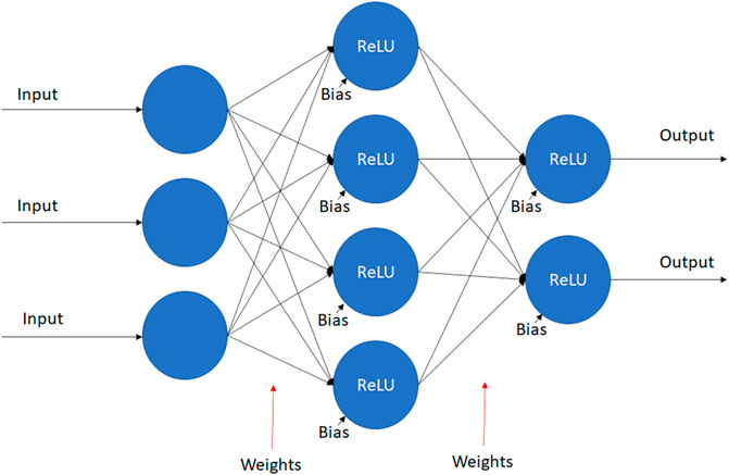
FIGURE 2. Schematic representation showing how the output is calculated in a two-layer artificial neural network where rectified linear unit (ReLU) is the activation function.

FIGURE 3. Representation of a residual block, where two layers are skipped.
Recurrent neural networks (RNN) [44] are DNNs designed for modeling time series. They use their own previous output hi−1 in combination with the input xi to calculate the next output:
Ideally the network learns to encode useful information in the output allowing the network to “remember” the past and predict better. We will be investigating the potential of using a long-short-term-memory (LSTM) netowrk [15], since they have exhibited very good performance [15]. One notable drawback with LSTMs is the fact that they are not designed for image analysis. Their memory requirements scales quadratically with input size, thus requiring to downsample the input. Therefore, we will investigate two networks, one including an LSTM and one without it, as discussed below. There are several possible choices for the activation function. In this work we use the rectified linear unit (ReLU) everywhere but the last layer, which has the form:
This activation function has been shown empirically to exhibit excellent performance in computer-vision problems [45]. We use the sigmoid activation function for the last layer to ensure that the output is in the range [0,1]. We will also use batch normalization [46], in particular the batch norm, which has been empirically proven to decrease training time and improve performance [47]. We use the first 800 fields as a training set and the remaining as a validation set. Our training and validation data is split into sequences of 16 fields each. The network accepts a sequence, and for each image in the sequence, predicts the following field in the time-series. All the hyper-parameters are tuned empirically, and Figure 4 shows the final architecture.
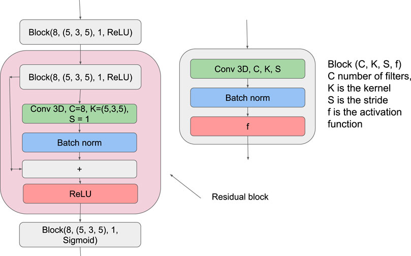
FIGURE 4. Schematic representation of the CNN architecture employed in this study.
We train our networks by minimizing the binary cross-entropy (BCE) between the predicted and the reference fields. To minimize training and inference discrepancy we will use the algorithm developed by Bengio et al. [48] during training. Thus, for a given sample of real fields, xi1, xi2, xi3, … , xim, the network will use the following algorithm:
Algorithm 1. :
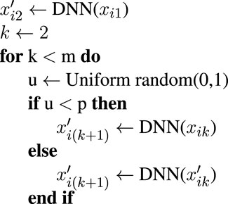 We anneal p at the speed of the inverse-sigmoid function parameter k = 30 during the training. At the start, the network will mostly make predictions based on actual data, while at the end, it will use its predictions. Several metrics are used for the evaluation of the network. We assessed the loss of the network during training to confirm that the network converges as expected. We are also interested in studying metrics such as the number of predicted structures in the field. Since the network is not outputting binary images but fields where every value is in the range [0, 1], we will apply rounding to the output. In this work, we use the algorithm described by Aguilar-Fuertes et al. [14] to identify structures and the volume of the minimum enclosing boxes.
Results
This study shows that the CNN-LSTM configuration, shown in Figure 5, exhibits poorer results. It only managed to learn the zero mapping, i.e. CNN-LSTM(x) = 0 ∀x. We hypothesize that this is caused by the field becoming too granular when downsampling so significantly. Thus, we will focus on the CNN architecture. Let us start by discussing the training process of the CNN configuration. In Figure 6 we show the training and validation losses, which decrease as expected. We observe that our validation loss starts above the training loss at around 50 steps but converges to a very similar value at around 200 steps. This significant loss difference is due to us testing in inference mode. The figure shows that the training loss becomes noisier at around 150 steps. This result is expected because as we predict farther into the future, we use more predicted samples rather than the ground truth, thus leading to the accumulation of errors. Interestingly, the training and validation losses reach the same value of 0.04 towards the end of the prediction horizon. Note that, although this could be indicative of under-fitting, using more complex models (i.e. deeper networks with more channels) did not produce any improvements in the results. We note that this is a highly chaotic problem, where instantaneous predictions are highly challenging, although the dynamic behavior of the flow can be predicted with excellent accuracy [23].
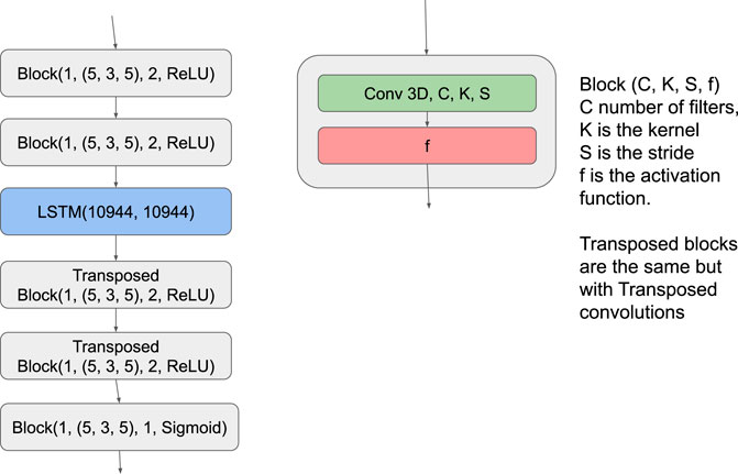
FIGURE 5. Schematic representation of the CNN-LSTM architecture employed in this study.
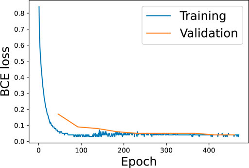
FIGURE 6. Training and validation binary-cross-entropy (BCE) losses for the CNN architecture as a function of the training epoch.
Next, we will assess the number (and the volume) of the coherent turbulent structures identified in the reference simulation and the predicted fields. Figures 7, 8 show the number of identified structures in the inner (y ≤ 0.2) and wake (y > 0.2) regions, respectively. The CNN architecture can accurately predict the evolution of the number of structures in time, with a small underestimation in the inner region and a slightly larger underestimation in the wake region. A plausible explanation for this result is that the network is conservative in its predictions. Consider the following scenario, where a point has a 10% chance of being part of a structure. The best possible guess would be a field of zeroes for a whole field, although it is doubtful that every point is zero. Similarly, the best prediction the network can make is likely zero for some points. In fact, these are the points near the edges of the structures that are the most challenging to predict. Thus we would expect the difference between predicted and real fields to grow proportionally to the number of structures. The data supports this explanation since the error is noticeably smaller when the number of structures is
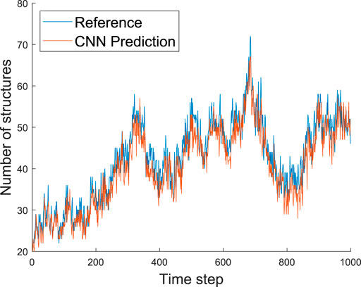
FIGURE 7. Predicted and reference number of structures as a function of the time step for the inner region, i.e. y ≤ 0.2. We observe that the number of structures is not constant over time.
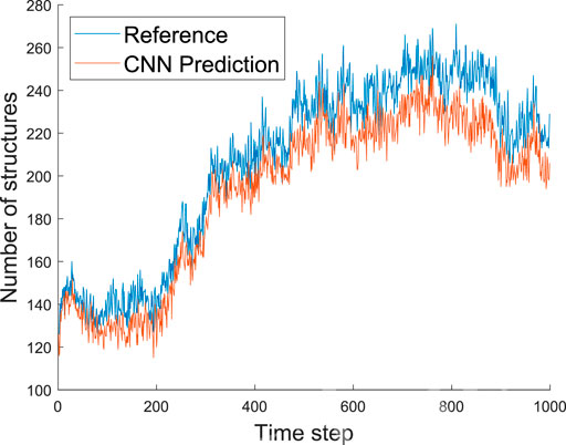
FIGURE 8. Predicted and reference number of structures as a function of the time step for the wake region, i.e. y > 0.2. We observe that the number of structures is not constant over time.
After predicting the number of structures in the turbulent fields, we analyze the volume of those objects. We show the evolution of the total volume of the structures in the inner and wake regions in Figures 9, 10, respectively. It can be observed that the employed CNN architecture exhibits excellent accuracy in the volume predictions. In the inner region, the only significant discrepancy we observe is at around step 400, while in the wake region, a discrepancy is observed around step 600. These deviations can be explained by the process to calculate the volume of the structures, which relies on the volume of the bounding box [13]. Note that a wrongly predicted zero value (i.e., no structure in that grid point) may have a significant effect if it disconnects a large structure. In this case, we will consider the volumes of two smaller boxes instead of the much larger volume of the complete bounding box. Interestingly, we do not see any network instance predicting a much larger volume than that of the real data. We expect the network to be slightly conservative for the same reasons outlined above, leading to underestimating the predicted volumes. In practice, the network only has to accurately predict the largest structures to obtain a correct prediction of the total volume. Furthermore, most of the time, these largest structures are not particularly sensitive to individual points. Thus, predicting the total volume is not a very challenging task.
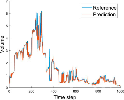
FIGURE 9. Predicted and reference volume (scaled with h3) of all the structures in the inner region (y ≤ 0.2) as a function of the time step. Note that the network rarely overestimates this volume.
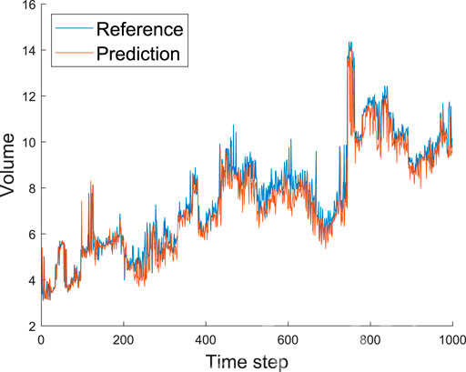
FIGURE 10. Predicted and reference volume (scaled with h3) of all the structures in the wake region (y > 0.2) as a function of the time step. Note that the network rarely overestimates this volume.
Finally, in Figure 11 we show the predicted and reference volumes of the largest structure in the domain as a function of the time step. Firstly, this figure shows that the largest structure is often responsible for over 50% of the total volume of all the structures in the domain. Interestingly, the CNN architecture exhibits very accurate results also when predicting the volume of the largest scales. Around time step 400, it can be observed that the volume difference between the predicted and real data is about one. The total volume difference supports our hypothesis that the (limited) discrepancies are associated with the calculation of the bounding-box volume. Furthermore, the sharp increase in maximum volume observed at around time step 750 is due to the merger of two different structures. All these results indicate that the CNN architecture can very accurately predict the geometrical properties of the structures, including the total number of objects and their volumes.
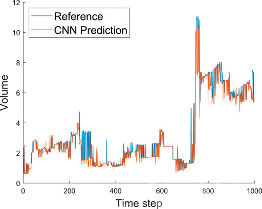
FIGURE 11. Predicted and reference volume (scaled with h3) of the largest structure in the domain as a function of the time step. Note that the sharp increase at around time step 750 matches the behavior in the wake region documented in Figure 10.
Discussion and Conclusion
In this work, we have designed a DNN capable of predicting the temporal evolution of the coherent structures in a turbulent channel flow. The employed CNN exhibits excellent agreement with the reference data, and some observed deviations are due to the method to calculate volumes based on bounding boxes. This also leads to scenarios where larger structures are responsible for a disproportionally large part of the total volume than their actual volume. Adding a single point to an edge of the structure is equivalent to adding a plane using this volume metric. Despite the mentioned caveats, this metric has been used to facilitate comparisons with other studies focused on coherent structures in turbulent channels. We also observe that the network predictions are conservative, with a general underprediction of the number of structures and their volume. This is associated with the rounding of the predictions: most points have a higher probability of being zero than one, and then the network will likely predict zero. This is not necessarily an issue, but future work will be focused on investigating the focal binary loss [50], to obtain a more even distribution. Note that our network shows signs of underfitting since the training and validation losses have approximately the same value. This was also the case in more complex networks investigated in this work. Overall, the performance of the CNN model is outstanding, with a satisfactory agreement between the predicted geometrical properties of the structures and those of the reference DNS data. In particular, throughout the whole time interval under study, our model leads to less than 2% error in the volume predictions and less than 0.5% in the predictions of number of structures.
When it comes to deep-learning models, including temporal information, we note the potential for further improving the predictions. This is because these models enable exploiting the spatial features in the data (as the CNN does) and the temporal correlations among snapshots, where multiple fields can be used as an input. In this work, we have also investigated adding a long-short-term-memory (LSTM) network [49] to handle the temporal information, although the significantly increased memory requirements of the new architecture limited its accuracy. Future work will aim at assessing more complicated architectures involving better downsampling, as in the U-net confgiration [50], or more efficient temporal networks such as temporal CNNs [51] or transformers [52].
Data Availability Statement
The raw data supporting the conclusion of this article will be made available by the authors, without undue reservation.
Author Contributions
DS performed the deep-learning analysis and wrote the paper; FA-A performed the simulations and edited the paper; SH performed the simulations and edited the paper; RV ideated the project, supervised and edited the paper.
Funding
RV acknowledges the financial support by the Göran Gustafsson foundation. SH was funded by Contract Nos. RTI2018-102256-B-I00 of Ministerio de Ciencia, innovación y Universidades/FEDER. Part of the analysis was carried out using computational resources provided by the Swedish National Infrastructure for Computing (SNIC).
Conflict of Interest
The authors declare that the research was conducted in the absence of any commercial or financial relationships that could be construed as a potential conflict of interest.
Publisher’s Note
All claims expressed in this article are solely those of the authors and do not necessarily represent those of their affiliated organizations, or those of the publisher, the editors and the reviewers. Any product that may be evaluated in this article, or claim that may be made by its manufacturer, is not guaranteed or endorsed by the publisher.
Acknowledgments
The authors thank Dr. H. Azizpour for his contributions on the deep-learning part of this work.
References
2. Vinuesa R, Brunton SL. The Potential of Machine Learning to Enhance Computational Fluid Dynamics. Preprint arXiv:2110.02085 (2021).
4. Hoyas S, Jiménez J. Scaling of the Velocity Fluctuations in Turbulent Channels up to Reτ=2003. Phys Fluids (2006) 18:011702. doi:10.1063/1.2162185
5. Hoyas S, Oberlack M, Alcántara-Ávila F, Kraheberger SV, Laux J. Wall Turbulence at High Friction reynolds Numbers. Phys Rev Fluids (2022) 7:014602. doi:10.1103/PhysRevFluids.7.014602
6. Noorani A, Vinuesa R, Brandt L, Schlatter P. Aspect Ratio Effect on Particle Transport in Turbulent Duct Flows. Phys Fluids (2016) 28:115103. doi:10.1063/1.4966026
7. Vinuesa R, Negi PS, Atzori M, Hanifi A, Henningson DS, Schlatter P. Turbulent Boundary Layers Around wing Sections up to Rec=1,000,000. Int J Heat Fluid Flow (2018) 72:86–99. doi:10.1016/j.ijheatfluidflow.2018.04.017
8. Abreu LI, Cavalieri AVG, Schlatter P, Vinuesa R, Henningson DS. Spectral Proper Orthogonal Decomposition and Resolvent Analysis of Near-wall Coherent Structures in Turbulent Pipe Flows. J Fluid Mech (2020) 900:A11. doi:10.1017/jfm.2020.445
9. Vinuesa R. High-fidelity Simulations in Complex Geometries: Towards Better Flow Understanding and Development of Turbulence Models. Results Eng (2021) 11:100254. doi:10.1016/j.rineng.2021.100254
10. Kline SJ, Reynolds WC, Schraub FA, Runstadler PW. The Structure of Turbulent Boundary Layers. J Fluid Mech (1967) 30:741–73. doi:10.1017/s0022112067001740
11. Ganapathisubramani B, Longmire EK, Marusic I. Characteristics of Vortex Packets in Turbulent Boundary Layers. J Fluid Mech (2003) 478:35–46. doi:10.1017/s0022112002003270
12. Gustavsson H. Introduction to Turbulence. Luleå: Division of Fluidmechanics, Luleå University of Technology (2006).
13. Lozano-Durán A, Flores O, Jiménez J. The Three-Dimensional Structure of Momentum Transfer in Turbulent Channels. J Fluid Mech (2012) 694:100–30. doi:10.1017/jfm.2011.524
14. Aguilar-Fuertes JJ, Noguero-Rodríguez F, Jaen Ruiz JC, García-RAffi LM, Hoyas S. Tracking Turbulent Coherent Structures by Means of Neural Networks. Energies (2021) 14:984. doi:10.3390/en14040984
15. Hochreiter S, Schmidhuber J. LSTM Can Solve Hard Long Time Lag Problems. In: MC Mozer, M Jordan, and T Petsche, editors. Advances in Neural Information Processing Systems, Vol. 9. Cambridge, MA, USA: MIT Press (1996).
16. Adrian RJ, Meinhart CD, Tomkins CD. Vortex Organization in the Outer Region of the Turbulent Boundary Layer. J Fluid Mech (2000) 422:1–54. doi:10.1017/s0022112000001580
17. del Álamo JC, Jiménez J, Zandonade P, Moser RD. Self-similar Vortex Clusters in the Turbulent Logarithmic Region. J Fluid Mech (2006) 561:329–58.
18. Jiménez J. Coherent Structures in wall-bounded Turbulence. J Fluid Mech (2018) 842:P1. doi:10.1017/jfm.2018.144
19. Rudin C. Stop Explaining Black Box Machine Learning Models for High Stakes Decisions and Use Interpretable Models Instead. Nat Mach Intell (2019) 1:206–15. doi:10.1038/s42256-019-0048-x
20. Vinuesa R, Sirmacek B. Interpretable Deep-Learning Models to Help Achieve the Sustainable Development Goals. Nat Mach Intell (2021) 3:926. doi:10.1038/s42256-021-00414-y
21. Bottou L. Stochastic Gradient Descent Tricks. In: Neural Networks: Tricks of the Trade. Berlin, Germany: Springer (2012). p. 421436–6. doi:10.1007/978-3-642-35289-8_25
22. Srinivasan PA, Guastoni L, Azizpour H, Schlatter P, Vinuesa R. Predictions of Turbulent Shear Flows Using Deep Neural Networks. Phys Rev Fluids (2019) 4:054603. doi:10.1103/physrevfluids.4.054603
23. Eivazi H, Guastoni L, Schlatter P, Azizpour H, Vinuesa R. Recurrent Neural Networks and Koopman-Based Frameworks for Temporal Predictions in Turbulence. Int J Heat Fluid Flow (2020) 90:108816.
24. Guastoni L, Güemes A, Ianiro A, Discetti S, Schlatter P, Azizpour H, et al. Convolutional-network Models to Predict wall-bounded Turbulence from wall Quantities. J Fluid Mech (2021) 928:A27. doi:10.1017/jfm.2021.812
25. Güemes A, Discetti S, Ianiro A, Sirmacek B, Azizpour H, Vinuesa R. From Coarse wall Measurements to Turbulent Velocity fields through Deep Learning. Phys Fluids (2021) 33:075121.
26. Eivazi H, Clainche SL, Hoyas S, Vinuesa R. Towards Extraction of Orthogonal and Parsimonious Non-linear Modes from Turbulent Flows. Preprint arXiv:2109.01514 (2021).
27. Jiang C, Vinuesa R, Chen R, Mi J, Laima S, Li H. An Interpretable Framework of Data-Driven Turbulence Modeling Using Deep Neural Networks. Phys Fluids (2021) 33:055133. doi:10.1063/5.0048909
28. Brunton SL, Noack BR, Koumoutsakos P. Machine Learning for Fluid Mechanics. Annu Rev Fluid Mech (2020) 52:477–508. doi:10.1146/annurev-fluid-010719-060214
29. Schmekel D. Predicting Coherent Turbulent Structures with. Master’s thesis. Stockholm, Sweden: KTH, Royal institute of technology (2022).
30. Lozano-Durán A, Jiménez J. Effect of the Computational Domain on Direct Simulations of Turbulent Channels up to Reτ = 4200. Phys Fluids (2014) 26:011702. doi:10.1063/1.4862918
31. Lluesma-Rodríguez F, Hoyas S, Peréz-Quiles M. Influence of the Computational Domain on DNS of Turbulent Heat Transfer up to Reτ = 2000 for Pr = 0.71. Int J Heat Mass Transfer (2018) 122:983–92.
32. Lluesma-Rodríguez F, Álcantara-Ávila F, Pérez-Quiles MJ, Hoyas S. A Code for Simulating Heat Transfer in Turbulent Channel Flow. Mathematics (2021) 9:756.
33. Avsarkisov V, Hoyas S, Oberlack M, García-Galache JP. Turbulent Plane Couette Flow at Moderately High reynolds Number. J Fluid Mech (2014) 751:R1. doi:10.1017/jfm.2014.323
34. Avsarkisov V, Oberlack M, Hoyas S. New Scaling Laws for Turbulent Poiseuille Flow with wall Transpiration. J Fluid Mech (2014) 746:99–122. doi:10.1017/jfm.2014.98
35. Kraheberger S, Hoyas S, Oberlack M. DNS of a Turbulent Couette Flow at Constant wall Transpiration up to. J Fluid Mech (2018) 835:421–43. doi:10.1017/jfm.2017.757
36. Alcántara-Ávila F, Hoyas S, Jezabel Pérez-Quiles M. Direct Numerical Simulation of thermal Channel Flow for and. J Fluid Mech (2021) 916:A29. doi:10.1017/jfm.2021.231
37. Oberlack M, Hoyas S, Kraheberger SV, Alcántara-Ávila F, Laux J. Turbulence Statistics of Arbitrary Moments of wall-bounded Shear Flows: A Symmetry Approach. Phys Rev Lett (2022) 128:024502. doi:10.1103/PhysRevLett.128.024502
38. Kim J, Moin P, Moser R. Turbulence Statistics in Fully Developed Channel Flow at Low Reynolds Number. J Fluid Mech (1987) 177:133–66. doi:10.1017/s0022112087000892
39. Lele SK. Compact Finite Difference Schemes with Spectral-like Resolution. J Comput Phys (1992) 103:16–42. doi:10.1016/0021-9991(92)90324-r
40. Spalart PR, Moser RD, Rogers MM. Spectral Methods for the Navier-Stokes Equations with One Infinite and Two Periodic Directions. J Comput Phys (1991) 96:297–324. doi:10.1016/0021-9991(91)90238-g
41. Gandía-Barberá S, Alcántara-Ávila F, Hoyas S, Avsarkisov V. Stratification Effect on Extreme-Scale Rolls in Plane Couette Flows. Phys Rev Fluids (2021) 6. doi:10.1103/PhysRevFluids.6.034605
42. Fukushima K, Miyake S. Neocognitron: A Self-Organizing Neural Network Model for a Mechanism of Visual Pattern Recognition. In: Competition and Cooperation in Neural Nets. Berlin, Germany: Springer (1982). p. 267–85. doi:10.1007/978-3-642-46466-9_18
43. He K, Zhang X, Ren S, Sun J. Deep Residual Learning for Image Recognition. In: Proceedings of the IEEE conference on computer vision and pattern recognition (2016). p. 770–8. doi:10.1109/cvpr.2016.90
45. Nwankpa C, Ijomah W, Gachagan A, Marshall S. Activation Functions: Comparison of Trends in Practice and Research for Deep Learning. arXiv preprint arXiv:1811.03378 (2018).
46. Ioffe S, Szegedy C. Batch Normalization: Accelerating Deep Network Training by Reducing Internal Covariate Shift. In: International conference on machine learning. New York City, NY, USA: PMLR (2015). p. 448–56.
47. Santurkar S, Tsipras D, Ilyas A, Madry A. How Does Batch Normalization Help Optimization? In: Proceedings of the 32nd international conference on neural information processing systems (2018). p. 2488–98.
48. Bengio S, Vinyals O, Jaitly N, Shazeer N. Scheduled Sampling for Sequence Prediction with Recurrent Neural Networks. arXiv preprint arXiv:1506.03099 (2015).
49. Lin T-Y, Goyal P, Girshick R, He K, Dollar P. Focal Loss for Dense Object Detection. In: Proceedings of the IEEE International Conference on Computer Vision (ICCV) (2017). doi:10.1109/iccv.2017.324
50. Ronneberger O, Fischer P, Brox T. U-net: Convolutional Networks for Biomedical Image Segmentation. In: International Conference on Medical image computing and computer-assisted intervention. Berlin, Germany: Springer (2015). p. 234–41. doi:10.1007/978-3-319-24574-4_28
51. Liu M, Zeng A, Lai Q, Xu Q. Time Series Is a Special Sequence: Forecasting with Sample Convolution and Interaction. CoRR abs/2106.09305 (2021).
Keywords: turbulence, coherent turbulent structures, machine learning, convolutional neural networks, deep learning
Citation: Schmekel D, Alcántara-Ávila F, Hoyas S and Vinuesa R (2022) Predicting Coherent Turbulent Structures via Deep Learning. Front. Phys. 10:888832. doi: 10.3389/fphy.2022.888832
Received: 03 March 2022; Accepted: 23 March 2022;
Published: 13 April 2022.
Edited by:
Traian Iliescu, Virginia Tech, United StatesReviewed by:
Omer San, Oklahoma State University, United StatesDiana Bistrian, Politehnica University of Timișoara, Romania
Copyright © 2022 Schmekel, Alcántara-Ávila, Hoyas and Vinuesa. This is an open-access article distributed under the terms of the Creative Commons Attribution License (CC BY). The use, distribution or reproduction in other forums is permitted, provided the original author(s) and the copyright owner(s) are credited and that the original publication in this journal is cited, in accordance with accepted academic practice. No use, distribution or reproduction is permitted which does not comply with these terms.
*Correspondence: R. Vinuesa, rvinuesa@mech.kth.se