Pattern Dynamics of Vegetation Growth With Saturated Water Absorption

Li, Li; Cao, Jia-Hui; Bao, Xin-Yue

doi:10.3389/fphy.2021.721115

ORIGINAL RESEARCH article

Front. Phys., 30 August 2021
Sec. Interdisciplinary Physics
Volume 9 - 2021 | https://doi.org/10.3389/fphy.2021.721115

Pattern Dynamics of Vegetation Growth With Saturated Water Absorption

Li Li^1,2* www.frontiersin.org

Jia-Hui Cao³ www.frontiersin.org

Xin-Yue Bao⁴

¹School of Computer and Information Technology, Shanxi University, Taiyuan, China
²Science and Technology on Electronic Test and Measurement Laboratory, North University of China, Taiyuan, China
³Complex Systems Research Center, Shanxi University, Taiyuan, China
⁴Yangzhou Shuren School, Yangzhou, China

Regular pattern is a typical feature of vegetation distribution and thus it is important to study the law of vegetation evolution in the fields of desertification and environment conservation. The saturated water absorption effect between the soil water and vegetation plays an crucial role in the vegetation patterns in semi-arid regions, yet its influence on vegetation dynamics is largely ignored. In this paper, we pose a vegetation-water model with saturated water absorption effect of vegetation. Our results show that the parameter 1/P, which is conversion coefficient of water absorption, has a great impact on pattern formation of vegetation: with the increase of P, the density of vegetation decrease, and meanwhile it can induce the transition of different patterns structures. In addition, we find that the increase of appropriate precipitation can postpone the time on the phase transition of the vegetation pattern. The obtained results systematically reveal the effect of saturated water absorption on vegetation systems which well enrich the findings in vegetation dynamics and thus may provide some new insights for vegetation protection.

1 Introduction

In nature, vegetation is very widely distributed in different places all over the world. At the same time, vegetation, as a producer in nature, converts carbon dioxide into carbohydrates through photosynthesis, which ensures the food source for humans and animals and keeps the content of carbon dioxide and oxygen in the environment relatively stable [1, 2]. Moreover, the soil and water conservation function of vegetation is also very significant. For example, vegetation can reduce the loss of rainwater on the surface and the erosion of the surface soil, and protect the sloping land. Vegetation stems and leaves release water vapor into the atmosphere by transpiration, so that water vapor emitted into the atmosphere and condensed water alleviates drought. Based on the above functions of vegetation, it is particularly necessary to study vegetation dynamics [3–6].

In recent years, duo to the impact of the greenhouse effect on human life and climate, vegetation plays an indispensable role in climate regulation [7, 8]. As for vegetation, people are always concerned about its growth and distribution. There are many factors affecting vegetation distribution, among which climate, geographical conditions and human factors are the most important. Moreover, different conditions will form different vegetation structure, and inhomogeneous distribution of vegetation is called vegetation pattern [9]. Pattern is a kind of non-uniform macroscopic structure with some regularity in space or time, which is ubiquitous in nature, such as stripes of clouds in the sky, waves on the water, figures on the animals and regular spatial pattern which observed in spatiotemporal systems far from equilibrium states [10, 11].

Patterns have been extensively studied and a wide range of patterns are found including vegetation patterns [12], infectious disease patterns [13], and patterns on predator-prey systems [14–16]. They are induced by different mechanisms and it is vital to understand these mechanisms. Mathematical modeling has become one of the most useful tools in exploring the mechanisms on vegetation dynamics including pattern formation and ecological functions [17]. There are many studies on vegetation pattern. In 1997, Lefever and Lejeune established a single-variable model, which revealed a resource competition mechanism among vegetation communities, namely promotion at short distance and inhibition at long distance [18]. In 1999, Klausmeier firstly proposed the classical vegetated-water model, explaining the regular stripes on the slopes and irregular mosaics on the ground, and pointed out that nonlinear mechanisms play a major role in determining the spatial structure of plant communities [19]. In 2013, Sun et al. revealed the relationship between precipitation and pattern formation: when rainfall is small, the vegetation will form spot pattern; when precipitation increases, the density of the spot pattern will increase, and vegetation appears as spot-stripes mixed pattern with low density [20]. In 2018, Liu et al. proposed a cross-diffusion vegetation system, in which the phenomenon of spot pattern transition was found [17]. In addition, cross-diffusion increased the vegetation density. In 2017, Zhang et al. proposed a vegetation-soil model and explained that wind can induce the generation of vegetation spot pattern. These models do not take into account that vegetation water absorption is not immoderate [21]. When vegetation water absorption reaches a certain degree, vegetation water absorption rate will decrease, which is called the saturation effect of vegetation water absorption. Yuval revealed that high water absorption and rapid diffusion of water in perennial herbs [22]. Of particular interest, this work showed that the pattern transition between multi-steady states is not necessarily catastrophic, yet it can be gradually phase-changed. Based on the observation data of mathematical model, the cause of fairy circles vegetation patch is explained as intra specific competition and the scale dependent effect of vegetation between animals that capture from plants [23]. There are also some work on the early warning signal of desertification [24–26].

Water absorption by vegetation is an important process of vegetation growth. The existed work assumed that water absorption is a linear function of vegetation biomass [6, 9, 19]. However, many types of vegetation have a saturation effect when absorbing water [27–30], which is generally not well studied by scientists. In fact, this saturated water absorption may have great influences of the vegetation pattern. In this sense, we will show the effect of saturation on the dynamical behavior of vegetation system.

The paper is organized as follows. In Section 2, we pose a vegetation-water model with saturated water absorption of vegetation and mathematical analysis on the emergence of Turing patterns is presented. In Section 3, we reveal the influences of saturated water absorption of vegetation on the patterns and persistence of vegetation system. In the last section, we give some discussion and conclusion.

2 Mathematical Analysis

In this section, we will introduce two-dimensional model to descrbe the interactions of vegetation and water, which is posed by Klausmeier [19]:

\{\begin{cases} \frac{\partial W}{\partial T} = A - L W - R W N^{2} + V \frac{\partial W}{\partial X}, \\ \frac{\partial N}{\partial T} = R J W N^{2} - M N + D Δ N . \end{cases} (1)

In the above model, there are seven parameters, which are used to depict vegetation physiological phenomena and the change of water. They are all positive depend on what the parameters mean. The first equation of the model (1) represents the change of water. A represents precipitation and water is reduced by evaporation at rate LW. Vegetation absorbs water at rate RG(W)F(N)N, where G(W) = W is saturated water absorption on vegetation, and take F(N) = N. The second equation of the model (1) is used to simulate the growth process of vegetation, where J is the conversion rate of vegetation into biomass through water absorption and M is lost through mortality. Water flow downhill at speed V and vegetation dispersal is modeled by a diffusion term with diffusion coefficient D.

In this work, we introduce a model contains two variables with saturated vegetation water absorption. This model is more reasonable compare with that model, in which the saturation of vegetation in absorbing water is not taken into account. It is because that the physiological process by which vegetation absorbs water from the soil and forms vegetation biomass is not inordinate, instead, as water increases, it is absorbed by vegetation to a state of saturation. 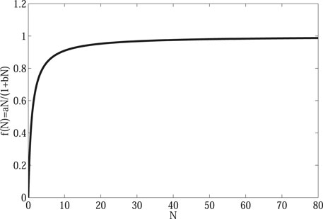Therefore, we take $F (N) = \frac{a N}{1 + b N}$ to model the saturated water absorption of vegetation (Figure 1).

FIGURE 1

FIGURE 1. Saturated water absorption on vegetation. When the water concentration is small, the water absorption of vegetation will increase with the increase of water concentration. However, as the water concentration continues to increase, the water absorption of vegetation tends to be constant.

At the same time, due to the diffusion of water, we will add $D_{1} Δ \bar{W}$ to our system, namely:

\{\begin{cases} \frac{\partial \bar{W}}{\partial \bar{T}} = A - L \bar{W} - R \bar{W} \frac{a {\bar{N}}^{2}}{1 + b \bar{N}} + D_{1} △ \bar{W}, \\ \frac{\partial \bar{N}}{\partial \bar{T}} = R J \bar{W} \frac{a {\bar{N}}^{2}}{1 + b \bar{N}} - M \bar{N} + D_{2} Δ \bar{N}, \end{cases} (2)

where the biological meanings and units of the parameters in system (2) can be found in Table 1.

TABLE 1

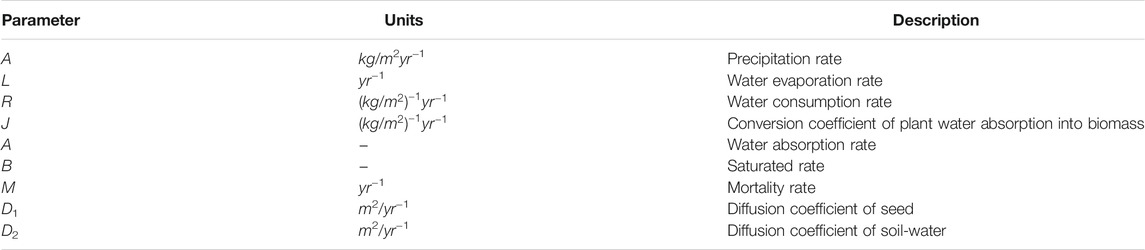
TABLE 1. Description of the parameters in the model (2).

Let

t = L \bar{T}, N = b \bar{N}, B = \frac{M}{L}, S = \frac{R J a A}{L^{2} b}, P = \frac{R a}{L b^{2}},

W = \frac{R J a}{L b} \bar{W}, x = \sqrt{\frac{b D_{2}}{L}} X, y = \sqrt{\frac{b D_{2}}{L}} Y, D = \frac{D_{1} R J a}{D_{2} L b^{2}} .

After the original system (2) is dimensionless, the following system is obtained:

\{\begin{cases} \frac{\partial W}{\partial t} = S - W - P \frac{W N^{2}}{1 + N} + D △ W, \\ \frac{\partial N}{\partial t} = \frac{W N^{2}}{1 + N} - B N + △ N . \end{cases} (3)

The initial conditions and boundary conditions are as follows:

W (x, y, 0) > 0, N (x, y, 0) > 0, (x, y) \in Ω = [0, L_{x}] \times [0, L_{y}], (4)

\frac{\partial W}{\partial \vec{n}} = \frac{\partial N}{\partial \vec{n}} = 0, (x, y) \in \partial Ω,

where L_x and L_y give region size in the directions of x and y respectively, $\vec{n}$ is the outward unit normal vector of the boundary ∂Ω, here we consider the boundary ∂Ω with no flux, namely, Neumann boundary [31–33].

In the absence of diffusion, we consider the following system:

\{\begin{cases} \frac{d W}{d t} = S - W - P \frac{W N^{2}}{1 + N} ≜ f (W, N), \\ \frac{d N}{d t} = \frac{W N^{2}}{1 + N} - B N ≜ g (W, N) . \end{cases} (5)

It is easy to gain that system (3) has a boundary equilibrium E₀ = (S, 0) and two positive equilibriums

E_{1} = (W_{1}, N_{1}) = (B + \frac{2 P B^{2}}{S - B + \sqrt{{(B - S)}^{2} - 4 P B^{2}}}, \frac{S - B + \sqrt{{(B - S)}^{2} - 4 P B^{2}}}{2 P B}),

E_{2} = (W_{2}, N_{2}) = (B + \frac{2 P B^{2}}{S - B - \sqrt{{(B - S)}^{2} - 4 P B^{2}}}, \frac{S - B - \sqrt{{(B - S)}^{2} - 4 P B^{2}}}{2 P B}) .

provided that

(1) S > B; (2) {(B - S)}^{2} - 4 P B^{2} > 0; (3) \sqrt{{(B - S)}^{2} - 4 P B^{2}} < S - B .

Under conditions (1), (2), (3), we focus on the stability of three equilibriums E₀, E₁, and E₂. The Jacobian matrix corresponding to equilibrium (W^∗, N^∗) as follows:

J = (\begin{matrix} a_{11} & a_{12} \\ a_{21} & a_{22} \end{matrix}),

where $a_{11} = - 1 - \frac{P N^{2}}{1 + N}, a_{12} = \frac{- 2 P W N}{1 + N} + \frac{P W N^{2}}{{(1 + N)}^{2}}, a_{21} = \frac{N^{2}}{1 + N}, a_{22} = \frac{2 W N}{1 + N} - \frac{W N^{2}}{{(1 + N)}^{2}}$ .

Then we can gain the linearized system:

\{\begin{cases} \frac{d W}{\partial t} = a_{11} W + a_{12} N, \\ \frac{d N}{\partial t} = a_{21} W + a_{22} N . \end{cases} (6)

And characteristic equation is:

λ^{2} - (a_{11} + a_{22}) λ + a_{11} a_{22} - a_{12} a_{21} = 0, (7)

where

- (a_{11} + a_{22}) = b_{1},

a_{11} a_{22} - a_{12} a_{21} = b_{2} .

i) When we consider E₀(S, 0), one can obtain

| λ E - J |_{E_{0}} = (λ + B) (λ + 1),

and thus it is clear that E₀(S, 0) is stable.

ii) When we consider E₁ = (W₁, N₁), then one can obtain the Jacobian matrix of system (5) at equilibrium E₁:

J |_{E_{1}} = (\begin{matrix} - 1 - \frac{P N_{1}^{2}}{1 + N_{1}} & - \frac{P B (N_{1} + 2)}{1 + N_{1}} \\ \frac{N_{1}^{2}}{1 + N_{1}} & \frac{B}{1 + N_{1}} \end{matrix}),

F (λ) |_{E_{1}} = | λ E - J ‖_{E_{1}} = λ^{2} + b_{11} λ + b_{12},

where

b_{11} = 1 + \frac{P N_{1}^{2} - B}{1 + N_{1}}, b_{12} = \frac{B (P N_{1}^{2} - 1)}{1 + N_{1}} .

Therefore the necessary and sufficient conditions for the equilibrium E₁ being stable is b₁₁ > 0 and b₁₂ > 0.

Now combining biological significance of each parameter, S > B holds. Then

b_{12} = \frac{△ + (S - B) \sqrt{△}}{S - B + \sqrt{△} + 2 P B} > 0,

where △ = (B−S)²− 4PB². In the following, we consider the sign of b₁₁,

b_{11} = 1 + \frac{{(S - B + \sqrt{△})}^{2} - 4 P B^{3}}{2 B (S - B + \sqrt{△} + 2 P B)} = 1 + \frac{△ + (S - B) \sqrt{△} + 2 P B^{2} (1 - B)}{B (S - B + \sqrt{△} + 2 P B)} .

When $S (S - B) + S \sqrt{Δ} > 2 P B^{3}$ , b₁₁ > 0 holds.

iii) Next, we investigate the stability of E₂ = (W₂, N₂). Similarly, we note the above equation as:

F_{2} (λ) = λ^{2} + b_{21} λ + b_{22},

b_{21} = 1 + \frac{P N_{2}^{2} - B}{1 + N_{2}}, b_{22} = \frac{B (P N_{2}^{2} - 1)}{1 + N_{2}} .

Substituting N₂ for b₂₁ and b₂₂, then we can obtain:

b_{21} = \frac{Δ - (S - B) \sqrt{Δ} + 2 P B (1 - B)}{B (S - B - \sqrt{Δ} + 2 P B)} + 1, b_{22} = \frac{Δ - (S - B) \sqrt{Δ}}{S - B - \sqrt{Δ} + 2 P B} .

Then analyzing the sign of b₂₁ and b₂₂. Because

\sqrt{Δ} = \sqrt{{(S - B)}^{2} - 4 P B^{2}} < S - B,

therefore b₂₂ < 0. So the equilibrium E₂ is unstable.

Therefore the system has only one stable positive equilibrium E₁. From biological perspective, we are interested in studying the stability behavior of E₁. The Jacobian matrix corresponding to E₁ is as follows:

J = (\begin{matrix} a_{111} & a_{112} \\ a_{121} & a_{122} \end{matrix}),

where

a_{11}^{*} = - 1 - \frac{{(S - B + \sqrt{Δ})}^{2}}{2 B (S - B + \sqrt{Δ} + 2 P B)} < 0,

a_{12}^{*} = - P B (1 + \frac{2 P B}{S - B + \sqrt{Δ} + 2 P B}) < 0,

a_{21}^{*} = - \frac{{(S - B + \sqrt{Δ})}^{2}}{2 P B (S - B + \sqrt{Δ} + 2 P B)} < 0,

a_{22}^{*} = \frac{2 P B^{2}}{S - B + \sqrt{Δ} + 2 P B} > 0 .

In the absence of diffusion, E₁ is stable, whereas become unstable when diffusion is added, which is called Turing instability.

\{\begin{cases} \frac{\partial W}{\partial t} = a_{11} W + a_{12} N + D Δ W, \\ \frac{\partial N}{\partial t} = a_{21} W + a_{22} N + Δ N . \end{cases} (8)

Nonuniform perturbation near the equilibrium point E₁:

(\begin{matrix} w \\ n \end{matrix}) = (\begin{matrix} w^{*} \\ n^{*} \end{matrix}) + ε (\begin{matrix} w_{k} \\ n_{k} \end{matrix}) e^{λ t + i k \vec{n}} + c \cdot c \cdot + O (ε^{2}), (9)

where λ is the growth rate of perturbations in time t, and i is the imaginary unit, k is the wave number, $\vec{r} = (x, y)$ is the spatial vector in two dimensional space and c. c. stands for the complex conjugate. Substituting (Eq. 9) into (Eq. 8), we obtain characteristic equation:

λ^{2} - t r (k) λ + △_{k} = 0,

where

\begin{align} t r_{k} = a_{11} + a_{22} - (1 + D) k^{2} = t r_{0} - k^{2} (1 + D), \end{align} (10a)

\begin{align} Δ_{k} = a_{11} a_{22} - a_{12} a_{21} - k^{2} (a_{11} + a_{22} D) + k^{4} D = Δ_{0} - k^{2} (a_{11} + a_{22} D) + k^{4} D . \end{align} (10b)

It is easy to get tr_k < 0 for any k due to that tr₀ < 0, while the sign of △k is indeterminate. Hopf bifurcation occurs when Im (λ₀) ≠ 0, Re (λ₀) = 0, that is a₁₁ + a₂₂ = 0, a₁₁a₂₂ − a₁₂a₂₁ > 0, then we obtain critical Hopf bifurcation curve a₁₁ + a₂₂ = 0. Then choosing S as Hopf bifurcation parameter, then

S_{H} = \frac{B^{2}}{B - 2}, (11)

Im (λ_k) = Re (λ_k) = 0 at k = k_T ≠ 0, that is $Δ_{k_{T}} = 0$ . And critical wave number satisfies

k_{T}^{2} = \frac{(a_{11} + a_{22} D)}{(2 D)} .

We take S as Turing bifurcation parameter, and its critical value S_T satisfies the following equation:

\begin{aligned} ((B^{2} D^{2} + 2 B D + 1) S^{4} \\ + P^{2} D^{4} B^{4} + 16 B^{3} P^{2} D^{3} - 20 B^{3} P D^{3} + 4 B^{3} D^{3} + 64 B^{2} P^{2} D^{2} - 16 B^{2} P D^{2} \\ + (26 B^{3} P D^{3} - 12 B^{3} D^{3} + 64 B^{2} P D^{2} - 8 B^{2} D^{2}) S \\ + (- 6 B^{3} P D^{3} + 12 B^{3} D^{3} - 14 B^{2} P D^{2} + 17 B^{2} D^{2} - 16 B P D + 4 B D) S^{2} \\ + (- 4 B^{3} D^{3} - 10 B^{2} D^{2} - 6 B D) S^{3}) B = 0 . \end{aligned}

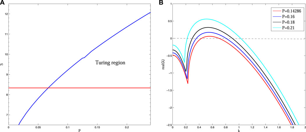
In this paper, taking D = 30, B = 5, we gain the Turing region of system (3). In this region, stationary patterns can be observed (Figure 2). In addition, we obtain the dispersion relation, and find that the real part of the eigenvalue $R (λ)$ increases as the value of P increases. Moreover, Turing pattern will appear within the appropriate parameter range. Dispersion relation shows that when there is no space, the equilibrium point E₁ is stable. When combined with space, loss of stability occurs in relation to the wave numbers. These curves reveal that saturated water absorption induces the instability of system (3).

FIGURE 2

FIGURE 2. (Color online) (A) The bifurcation diagram for system (3) in P—S plane. In Turing region, Turing pattern will form. (B) Dispersion relation of system (3) with different P, other parameter values are taken as: S = 10, B = 5, D = 30, which reveals that the real-part of eigenvalues $R (λ)$ increases with P increasing.

3 Multiple Scale Analysis for Turing Patterns

The standard multiple-scale analysis yields the well-known amplitude equations. Close to the onset S = S_T, the eigenvalues associated to the critical modes are close to zero, and they are slowly varying modes, whereas the off-critical mode relax quickly [15, 34]. Consequently, the whole dynamical behaviors can be mainly determined by the dynamics of the active slow modes. The stability and the selection of the different patterns close to onset can be derived from the amplitude equations that govern the dynamics of these active modes. Turing patterns (e.g., hexxagon and stripe patterns) are thus well described by a system of three active resonant pair of modes (k_j,−k_j) (j = 1, 2, 3) making angles of $\frac{2 π}{3}$ and |k_j = k_T|. We obtain the linearized form of model (3) at the equilibrium point E₁ as follows:

(\begin{matrix} \frac{\partial x}{\partial t} = a_{11} x + a_{12} y - \frac{P N^{*} (N^{*} + 2)}{{(1 + N^{*})}^{2}} x y - \frac{P W^{*}}{{(1 + N^{*})}^{3}} y^{2} - \frac{P}{{(1 + N^{*})}^{3}} x y^{2} + \frac{P W^{*}}{{(1 + N^{*})}^{4}} y^{3} + D Δ x, \\ \frac{\partial y}{\partial t} = a_{21} x + a_{22} y + \frac{N^{*} (N^{*} + 2)}{{(1 + N^{*})}^{2}} x y + \frac{W^{*}}{{(1 + N^{*})}^{3}} y^{2} + \frac{1}{{(1 + N^{*})}^{3}} x y^{2} - \frac{W^{*}}{{(1 + N^{*})}^{4}} y^{3} + Δ y . \end{matrix} (12)

We note

a_{13} = - \frac{P N^{*} (N^{*} + 2)}{{(1 + N^{*})}^{2}}; a_{14} = - \frac{P W^{*}}{{(1 + N^{*})}^{3}}; a_{15} = - \frac{P}{{(1 + N^{*})}^{3}}; a_{16} = \frac{P W^{*}}{{(1 + N^{*})}^{4}};

a_{23} = \frac{N^{*} (N^{*} + 2)}{{(1 + N^{*})}^{2}}; a_{24} = \frac{W^{*}}{{(1 + N^{*})}^{3}}; a_{25} = \frac{1}{{(1 + N^{*})}^{3}}; a_{26} = - \frac{W^{*}}{{(1 + N^{*})}^{4}};

and we will gain:

(\begin{matrix} \frac{\partial x}{\partial t} = a_{11} x + a_{12} y + a_{13} x y + a_{14} y^{2} + a_{15} x y^{2} + a_{16} y^{3} + D Δ x, \\ \frac{\partial y}{\partial t} = a_{21} x + a_{22} y + a_{23} x y + a_{24} y^{2} + a_{25} x y^{2} + a_{26} y^{3} + Δ y . \end{matrix} (13)

Close to onset S = S_T, the solutions of model (5a) (5b) can be expanded as

U = U_{S} + Σ_{j = 1}^{3} U_{0} [A_{j} e x p (i k_{j} \cdot \vec{r}) + \bar{A_{j}} e x p (- i k_{j} \cdot \vec{r})] . (14)

At the same time, the solution of model (12) can be expanded as

U^{0} = Σ_{j = 1}^{3} U_{0} [A_{j} e x p (i k_{j} \cdot \vec{r}) + \bar{A_{j}} e x p (- i k_{j} \cdot \vec{r})], (15)

where U_S represents the uniform steady state. A_j and the conjugate ${\bar{A}}_{j}$ are the amplitudes associated with the modes k_j and −k_j, respectively. The amplitude equations are described through the equations:

(\begin{matrix} τ_{0} \frac{\partial A_{1}}{d t} = μ A_{1} + h {\bar{A}}_{2} {\bar{A}}_{3} - (g_{1} | A_{1} |^{2} + g_{2} (| A_{2} |^{2} + | A_{3} |^{2})) A_{1}, \\ τ_{0} \frac{\partial A_{2}}{d t} = μ A_{2} + h {\bar{A}}_{1} {\bar{A}}_{3} - (g_{1} | A_{2} |^{2} + g_{2} (| A_{1} |^{2} + | A_{3} |^{2})) A_{2}, \\ τ_{0} \frac{\partial A_{3}}{d t} = μ A_{3} + h {\bar{A}}_{1} {\bar{A}}_{2} - (g_{1} | A_{3} |^{2} + g_{2} (| A_{1} |^{2} + | A_{2} |^{2})) A_{3} . \end{matrix} (16)

where μ = (S_T − S)/S_T is a normalized distance to onset, τ₀ is a typical relaxation time. In the following, we will give the exact expressions of the coefficient τ₀, h, g₁ and g₂. Setting X = (x, y)^T, N = (N₁, N₂), model (12) can be converted to the following system:

\frac{\partial X}{\partial t} = L X + N, (17)

where

L = (\begin{matrix} a_{11} + D Δ & a_{12} \\ a_{21} & a_{22} + Δ \end{matrix}),

(\begin{matrix} N_{1} \\ N_{2} \end{matrix}) (\begin{matrix} - \frac{P N^{*} (N^{*} + 2)}{{(1 + N^{*})}^{2}} x y - \frac{P W^{*}}{{(1 + N^{*})}^{3}} y^{2} - \frac{P}{{(1 + N^{*})}^{3}} x y^{2} + \frac{P W^{*}}{{(1 + N^{*})}^{4}} y^{3} \\ \frac{N^{*} (N^{*} + 2)}{{(1 + N^{*})}^{2}} x y + \frac{W^{*}}{{(1 + N^{*})}^{3}} y^{2} + \frac{1}{{(1 + N^{*})}^{3}} x y^{2} - \frac{W^{*}}{{(1 + N^{*})}^{4}} y^{3} \end{matrix}) .

During the calculation, we just analysis the behavior of the parameter close to onset S = S_T. With this method, we can expanded S in the following term:

S_{T} - S = ε S_{1} + ε^{2} S_{2} + ε^{3} S_{3} + O (ε^{4}), (18)

where ɛ is a small parameter. Expanding the variable X and the nonlinear term N according to this small parameter, we have the following results:

X = (\begin{matrix} x \\ y \end{matrix}) = ε (\begin{matrix} x_{1} \\ y_{1} \end{matrix}) + ε^{2} (\begin{matrix} x_{2} \\ y_{2} \end{matrix}) + O (ε^{3}), (19)

N = ε^{2} h^{2} + ε^{3} h^{3} + O (ε^{4}) . (20)

where h² and h³ are corresponding to the second and the third order of ɛ in the expansion of the nonlinear term N. At the same time, the linear operator L can be expanded as follows:

L = L_{T} + (S_{T} - S) M, (21)

where

L_{T} = (\begin{matrix} a_{11}^{*} + D Δ & a_{12}^{*} \\ a_{21}^{*} & a_{22}^{*} + Δ \end{matrix}),

M = (\begin{matrix} \frac{a_{11} - a_{11}^{*}}{S_{T} - S} & \frac{a_{12} - a_{12}^{*}}{S_{T} - S} \\ \frac{a_{21} - a_{21}^{*}}{S_{T} - S} & \frac{a_{22} - a_{22}^{*}}{S_{T} - S} \end{matrix}) = (\begin{matrix} m_{11} & m_{12} \\ m_{21} & m_{22} \end{matrix}) .

Here one can have the expression of $a_{i j}^{*}$ by substituting A_T for A in a_ij and b_ij is easy to be obtained. As for multiple-scale analysis, what really pivotal is that we can separate the dynamic behavior according to different time or spatial scale. We only need to separate the time scale for model (16) (i.e., T₀ = t, T₁ = ɛt, T₂ = ɛ²t). Each time scale T_i can be considered as independent variable. The derivative with respect to time becomes the following form:

\frac{\partial}{\partial t} = \frac{\partial}{\partial T_{0}} + ε \frac{\partial}{\partial T_{1}} + ε^{2} \frac{\partial}{\partial T_{2}} + O (ε^{3}) . (22)

Since that amplitude A is a variable that changes slowly, the derivative with respect to time $\frac{\partial}{\partial T_{0}}$ , which changes fast does not effect on the amplitude A. As a result, we have the following result:

\frac{\partial A}{\partial t} = ε \frac{\partial A}{\partial T_{1}} + ε^{2} \frac{\partial A}{\partial T_{2}} + O (ε^{3}) . (23)

By using the Eq. 19, Eq. 20, Eq. 21, Eq. 22, and expanding Eq. 15. according to different orders of ɛ, we can obtain three equations as follows: The first order of ɛ:

L_{T} (\begin{matrix} x_{1} \\ y_{1} \end{matrix}) = 0;

The second order of ɛ:

L_{T} (\begin{matrix} x_{2} \\ y_{2} \end{matrix}) = \frac{\partial}{\partial T_{1}} (\begin{matrix} x_{1} \\ y_{1} \end{matrix}) - S_{1} M (\begin{matrix} x_{1} \\ y_{1} \end{matrix}) - (\begin{matrix} \frac{- P N^{*} (N^{*} + 2)}{{(1 + N^{*})}^{2}} x y - \frac{P W^{*}}{{(1 + N^{*})}^{3}} y^{2} \\ \frac{N^{*} (N^{*} + 2)}{{(1 + N^{*})}^{2}} x y + \frac{W^{*}}{{(1 + N^{*})}^{3}} y^{2} \end{matrix});

The third order of ɛ:

L_{T} (\begin{matrix} x_{3} \\ y_{3} \end{matrix}) = \frac{\partial}{\partial T_{1}} (\begin{matrix} x_{2} \\ y_{2} \end{matrix}) + \frac{\partial}{\partial T_{2}} (\begin{matrix} x_{1} \\ y_{1} \end{matrix}) - S_{1} M (\begin{matrix} x_{2} \\ y_{2} \end{matrix}) - S_{2} M (\begin{matrix} x_{1} \\ y_{1} \end{matrix}) - Z,

Z = (\begin{matrix} \frac{- P N^{*} (N^{*} + 2)}{{(1 + N^{*})}^{2}} (x_{1} y_{2} + x_{2} y_{1}) - \frac{2 P W^{*}}{{(1 + N^{*})}^{3}} y_{1} y_{2} - \frac{P}{{(1 + N^{*})}^{3}} x_{1} y_{1}^{2} + \frac{P W^{*}}{{(1 + N^{*})}^{4}} y_{1}^{3} \\ \frac{N^{*} (N^{*} + 2)}{{(1 + N^{*})}^{2}} (x_{1} y_{2} + x_{2} y_{1}) + \frac{2 W^{*}}{{(1 + N^{*})}^{3}} y_{1} y_{2} + \frac{1}{{(1 + N^{*})}^{3}} x_{1} y_{1}^{2} - \frac{W^{*}}{{(1 + N^{*})}^{4}} y_{1}^{3} \end{matrix}) .

As for the first order of ɛ:

L_{T} (\begin{matrix} x_{1} \\ y_{1} \end{matrix}) = 0, (24)

as L_T is the linear operator of the system close to the onset, ${(x_{1}, y_{1})}^{T}$ is the linear combination of the eigenvectors that corresponding to the eigenvalue 0. Solving the first order of ɛ, we can obtain:

(\begin{matrix} x_{1} \\ y_{1} \end{matrix}) = (\begin{matrix} l \\ 1 \end{matrix}) (W_{1} e^{i k_{1} \vec{r}} + W_{2} e^{i k_{2} \vec{r}} + W_{3} e^{i k_{3} \vec{r}}) + c . c ., (25)

where $| k_{j} | = k_{T}^{*}$ , $l = \frac{a_{11}^{*} - a_{22}^{*} D}{2 a_{12}^{*} D}$ . W_j is the amplitude of the mode $e^{i k_{j} \vec{r}}$ when the system is under the first order perturbation.

For the second order of ɛ, we can obtain:

L_{T} (\begin{matrix} x_{2} \\ y_{2} \end{matrix}) = \frac{\partial}{\partial T_{1}} (\begin{matrix} x_{1} \\ y_{1} \end{matrix}) - S_{1} M (\begin{matrix} x_{1} \\ y_{1} \end{matrix}) - (\begin{matrix} \frac{- P N^{*} (N^{*} + 2)}{{(1 + N^{*})}^{2}} x y - \frac{P W^{*}}{{(1 + N^{*})}^{3}} y^{2} \\ \frac{N^{*} (N^{*} + 2)}{{(1 + N^{*})}^{2}} x y + \frac{W^{*}}{{(1 + N^{*})}^{3}} y^{2} \end{matrix}) = (\begin{matrix} F_{x} \\ F_{y} \end{matrix}) . (26)

According to the Fredholm solubility condition, the vector function of the right hand of Eq. 25. must be orthogonal with the zero eigenvectors of operator $L_{c}^{+}$ , where $L_{c}^{+}$ is the adjoint operator of $L_{c}^{+}$ . In this system, the zero eigenvectors of operator $L_{c}^{+}$ are

(\begin{matrix} 1 \\ - l D \end{matrix}) e^{- i k_{j} \vec{r}} + c . c . (j = 1,2,3) (27)

The orthogonality condition is

(\begin{matrix} 1, - l D \end{matrix}) (\begin{matrix} F_{x}^{i} \\ F_{y}^{i} \end{matrix}) = 0, (28)

where $F_{x}^{i}$ and $F_{y}^{i}$ , separately, represent the coefficients corresponding to $e^{i k_{j} \vec{r}}$ in F_x and F_y. Taking $e^{i k_{1} \vec{r}}$ for instance, we will gain

l (1 - D) \frac{\partial W_{1}}{\partial T_{1}} = S_{1} [(m_{11} l + m_{12}) - l D (m_{21} l + m_{22})] W_{1} + 2 [(a_{13} l + a_{14}) - l D (a_{23} l + a_{24})] {\bar{W}}_{2} {\bar{W}}_{3} . (29)

The coefficient in Eq. 30. are obtained by solving the sets of the linear equations about exp (0), $e x p (i k_{j} \vec{r})$ , $e x p (i 2 k_{j} \vec{r})$ , $e x p (i (k_{j} - k_{k}) \vec{r})$ .

With this method, we have

(\begin{matrix} X_{0} \\ Y_{0} \end{matrix}) = (\begin{matrix} f_{0} \\ g_{0} \end{matrix}) (| W_{1} |^{2} + | W_{2} |^{2} + | W_{3} |^{2}),

X_{i} = l Y_{i},

(\begin{matrix} X_{j j} \\ Y_{j j} \end{matrix}) = (\begin{matrix} s \\ t \end{matrix}) W_{j}^{2},

(\begin{matrix} X_{j k} \\ Y_{j k} \end{matrix}) = (\begin{matrix} p \\ q \end{matrix}) W_{j} {\bar{W}}_{k},

For the third order, we can gain

L_{T} (\begin{matrix} x_{3} \\ y_{3} \end{matrix}) = \frac{\partial}{\partial T_{1}} (\begin{matrix} x_{2} \\ y_{2} \end{matrix}) + \frac{\partial}{\partial T_{2}} (\begin{matrix} x_{1} \\ y_{1} \end{matrix}) - S_{1} M (\begin{matrix} x_{2} \\ y_{2} \end{matrix}) - S_{2} M (\begin{matrix} x_{1} \\ y_{1} \end{matrix}) - Z . (30)

Using the Fredholm solubility condition again, we can obtain

\begin{aligned} l (1 - D) [\frac{\partial W_{1}}{\partial T_{2}} + \frac{\partial Y_{1}}{\partial T_{1}}] \\ = S_{1} [(m_{11} l + m_{12}) - l D (m_{21} l + m_{22})] Y_{1} + S_{2} [(m_{11} l + m_{12}) - l D (m_{21} l + m_{22})] W_{1} \\ + 2 [(a_{13} l + a_{14}) - l D (a_{23} l + a_{24})] ({\bar{Y}}_{2} {\bar{W}}_{3} + {\bar{Y}}_{3} {\bar{W}}_{2}) \\ - (G_{1} | W_{1} |^{2} + G_{2} (| W_{2} |^{2} + | W_{3} |^{2})) W_{1}, \end{aligned}

where

G_{1} = (a_{13} - l D a_{23}) (l g_{0} + f_{0}) + 6 [(a_{15} l + a_{16}) - l D (a_{25} l + a_{26})]

G_{2} = (a_{13} - l D a_{23}) (l g_{0} + f_{0}) + 9 [(a_{15} l + a_{16}) - l D (a_{25} l + a_{26})]

By transformation of W, the other two equations can be obtained and the amplitude A_i can be expanded as

A_{i} = ε W_{i} + ε^{2} Y_{i} + O (ε^{3}) . (31)

For the order ɛ² and ɛ³, we can obtain the amplitude equation corresponding to A₁ as follows:

τ_{0} \frac{\partial A_{1}}{\partial t} = μ A_{1} + h {\bar{A}}_{2} {\bar{A}}_{3} - (g_{1} | A_{1} |^{2} + g_{2} (| A_{2} |^{2} + | A_{3} |^{2})) A_{1}, (32)

where

τ_{0} = \frac{l}{H} S_{T} (1 - D), μ = \frac{S_{T} - S}{S_{T}}, h = \frac{2 C}{l H S_{T}},

g_{1} = \frac{G_{1} S_{T}}{H l^{2}}, g_{2} = \frac{G_{2} S_{T}}{H l^{2}} .

with H = [(m₁₁l + m₁₂) − lD (m₂₁l + m₂₂)], C = 2 [(a₁₃l + a₁₄) − lD (a₂₃l + a₂₄)].

The other two equations we can gain by transforming the subscript of A. Based on Ref. [10], one can calculate the values of μ_i (i = 1, 2, 3, 4). When the controlled parameter μ increase to the critical point μ₂ = 0, the stationary state of the system begins to lose stability. If μ₁ < μ < μ₂, then the system exists a bistable region in the range of the controlled parameter. The emergence of Stripe patterns derives from supercritical bifurcation which are unstable for μ < μ₃ and stable for μ > μ₃. When the controlled parameter μ exceed μ₄, there is coexistence of hexagon and stripe pattern.

4 Main Results

In order to verify the above theoretical results, we carry out numerical simulation by taking B = 5, D = 30, and S = 10. This paper focuses on the spatial distribution of vegetation with the change of parameter P.

Currently, the desertification phenomenon is particularly austere, so it is the fundamental way for people to understand the cause of desertification correctly to master the law of vegetation evolution [35, 36].

Figure 3 shows the evolution of the spatial pattern of vegetation at 0, 1,000, 2000, 4,000, 10,000 and 20,000 iterations with p = 0.15. In (A), the vegetation distribution presents an irregular uniform mixing state, and the vegetation is uniformly distributed in the two-dimensional space. Then in (B), the vegetation can be observed to begin to gather into spot and stripe, but the density is not high. With time going by, in (C), the vegetation density increased. In (D), the spatial distribution of vegetation changes, forming a low-density stripe state. However, in (E), the structure of vegetation changes from low density stripe to higher stripe state gradually. At last, in (F), the density of the mixed pattern increases to form a clearer mixed pattern, and it doesn’t change for a long time. The above figures show the change and evolution of vegetation structure over time. It can be concluded from this figure that random distribution can result in mixed patterns.

FIGURE 3

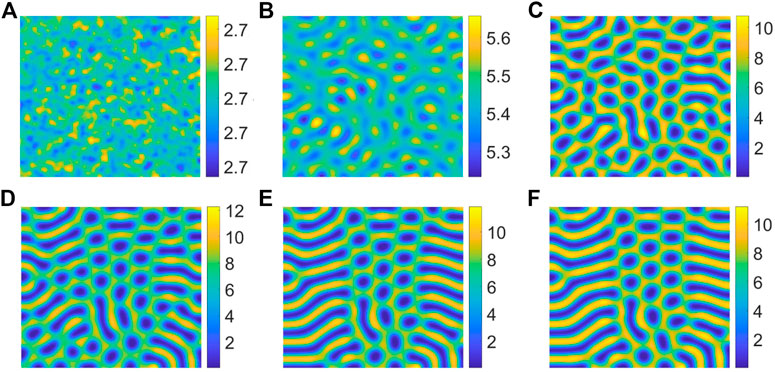
FIGURE 3. Snapshots of contour pictures of the time evolution of vegetation at different instants with p = 0.15, S = 10, D = 30 and B = 5. (A) 0 iteration; (B) 1,000 iterations; (C) 2000 iterations; (D) 4,000 iterations; (E) 10,000 iterations; (F) 20,000 iterations.

In Figure 4, we can find that the pattern is self-organizing. When the parameter(P) describing the saturated water absorption of vegetation changes, self-organizing patterns of different states can be obtained. Figure 4 shows the transition of the vegetation pattern with p = 0.14286, 0.15, 0.16, 0.18, 0.21 and 0.22, where B = 5, D = 30, S = 10. From the simulation results of Figure 5, we can conclude that vegetation density get smaller and smaller with P increasing, which is consistent with the fact that 1/P is proportional to the rate at which vegetation absorbs water to generate vegetation. Meanwhile, we can find that the pattern changes from honeycomb pattern to mixed pattern, then changes from mixed pattern to labyrinth pattern, at last pattern changes from labyrinth pattern to spot pattern. As a result, we can conclude that the change of P induces pattern phase transition. Many researchers have proposed that spot pattern is the early warning of desertification [31, 37, 38], therefore we can get that P is of great significance in indicating desertification. Moreover, from the tendency of pattern phase transition, it can be found that P also has a vital influence on the ecosystem robustness. The larger P is, the more unstable the system tends to be. In general, the bigger vegetation density corresponds to a more robust ecosystem.

FIGURE 4

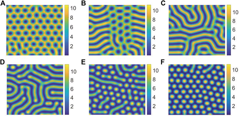
FIGURE 4. Snapshots of the countour pictures of evolution of vegetation with different values of P, (A) p = 0.14286; (B) p = 0.15; (C) p = 0.16; (D) p = 0.18; (E) p = 0.21; (F) p = 0.22. The other parameters are taken as S = 10, B = 5, and D = 30.

FIGURE 5

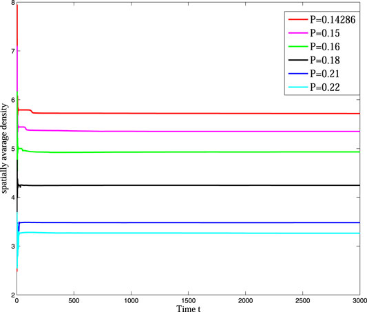
FIGURE 5. (Color online) The time series of vegetation with P taking different values.

It is well known that precipitation plays a very significant role in vegetation growth. However, the relationship between precipitation and saturated water absorption of vegetation is still unclear. To reveal the relationship between them, we take S = 10.5, B = 5 and D = 30 and perform simulations. Then we gain the effect of P on the pattern phase transition and find several types of typical patterns in Figure 6.

FIGURE 6

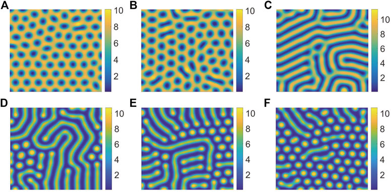
FIGURE 6. Snapshots of the countour pictures of evolution of vegetation with different values of P, (A) p = 0.16; (B) p = 0.17; (C) p = 0.18; (D) p = 0.23; (E) p = 0.238; (F) p = 0.25. The other parameters are taken as S = 10.5, B = 5, and D = 30.

On the circumstance of the increase of S, the pattern phase transition is insensitive to P. That is to say, when P changes from 0.1428 to 0.15 with S = 10, the pattern structure changes from honeycomb pattern to mixed pattern, however, when S = 10.5, the same transition tendency of which pattern structure from honeycomb pattern to mixed pattern will need a change of P from 0.16 to 0.23. Of course, the increase of the value of precipitation also increases the density of vegetation (Figure 7).

FIGURE 7

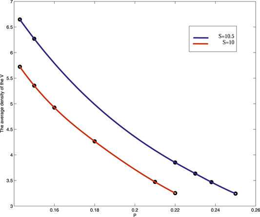
FIGURE 7. (Color online) The average density map of vegetation is compared when precipitation is taken S = 10 and S = 10.5 respectively.

5 Conclusion

In this work, we show the effect of saturated water absorption on the vegetation dynamics based on a mathematical model in the form of reaction-diffusion equations. We gain rich pattern structures including spotted, mixed, stripe, honeycomb, and labyrinth patterns. It is revealed that there is a negative correlation between P and vegetation density. That is to say, the vegetation biomass decreases as the increase of P, and saturated water absorption can induces the pattern transition of vegetation structures in two-dimensional space. In addition, we also conclude that appropriate precipitation increase can postpone the pattern phase transition.

In this work, we focused our attention on the influences of parameter change on the dynamical behaviors. The results showed that small change may induce the behavior shift between different dynamical regions [39]. The findings can also be applied in other related fields, such as ecosystems, disease transmission, evolutions and so on.

It needs to point out that climatic factors are important impact factors for vegetation dynamics [40, 41]. In this sense, we need to combine these factors including temperature, illumination and wind to the mathematical models. Furthermore, big data analysis is useful to explore the inherent law of vegetation evolution in both space and time [42, 43]. These topics will be well addressed in the further study.

Data Availability Statement

The original contributions presented in the study are included in the article/Supplementary Material, further inquiries can be directed to the corresponding author.

Author Contributions

All authors have made great contributions to the writing of study and approved the submitted version. LL, J-HC, and X-YB established dynamical modeling. LL and J-HC participated in the program design. LL and X-YB mainly wrote the manuscript.

Funding

The project is funded by the National Natural Science Foundation of China under Grant No. 42075029, Program for the Outstanding Innovative Teams (OIT) of Higher Learning Institutions of Shanxi, and China Postdoctoral Science Foundation under Grant Nos. 2017M621110 and 2019T120199.

Conflict of Interest

The authors declare that the research was conducted in the absence of any commercial or financial relationships that could be construed as a potential conflict of interest.

Publisher’s Note

All claims expressed in this article are solely those of the authors and do not necessarily represent those of their affiliated organizations, or those of the publisher, the editors and the reviewers. Any product that may be evaluated in this article, or claim that may be made by its manufacturer, is not guaranteed or endorsed by the publisher.

References

1. Porporato A, D'Odorico P, Laio F, Ridolfi L, Rodriguez-Iturbe I. Ecohydrology of Water-Controlled Ecosystems. Adv Water Resour (2002) 25:1335–48. doi:10.1016/S0309-1708(02)00058-1

CrossRef Full Text

2. Morgan RPC, Duzant JH. Modified MMF (Morgan-Morgan-Finney) Model for Evaluating Effects of Crops and Vegetation Cover on Soil Erosion. Earth Surf Process Landforms (2008) 33:90–106. doi:10.1002/esp.1530

CrossRef Full Text | Google Scholar

3. Balke T, Herman PMJ, Bouma TJ. Critical Transitions in Disturbance-Driven Ecosystems: Identifying Windows of Opportunity for Recovery. J Ecol (2014) 102:700–8. doi:10.1111/1365-2745.12241

CrossRef Full Text | Google Scholar

4. Claussen M, Bathiany S, Brovkin V, Kleinen T. Simulated Climate-Vegetation Interaction in Semi-arid Regions Affected by Plant Diversity. Nat Geosci (2013) 6:954–8. doi:10.1038/ngeo1962

CrossRef Full Text | Google Scholar

5. Juergens N. The Biological Underpinnings of Namib Desert Fairy Circles. Science (2013) 339:1618–21. doi:10.1126/science.1222999

PubMed Abstract | CrossRef Full Text | Google Scholar

6. Getzin S, Yizhaq H, Bell B, Erickson TE, Postle AC, Katra I, et al. Discovery of Fairy Circles in Australia Supports Self-Organization Theory. Proc Natl Acad Sci USA (2016) 113:3551–6. doi:10.1073/pnas.1522130113

PubMed Abstract | CrossRef Full Text | Google Scholar

7. Anselmo C, Thomas B, Miffre A, Francis M, Cariou JP, Rairoux P. Remote Sensing of Greenhouse Gases by Combining Lidar and Optical Correlation Spectroscopy. EPJ Web of Conferences (2016) 119:05007. doi:10.1051/epjconf/201611905007

CrossRef Full Text | Google Scholar

8. Giorgi F. Uncertainties in Climate Change Projections, from the Global to the Regional Scale. EPJ Web of Conferences (2010) 9:115–29. doi:10.1051/epjconf/201009009

CrossRef Full Text | Google Scholar

9. Sun G-Q, Wang C-H, Chang L-L, Wu Y-P, Li L, Jin Z. Effects of Feedback Regulation on Vegetation Patterns in Semi-arid Environments. Appl Math Model (2018) 61:200–15. doi:10.1016/j.apm.2018.04.010

CrossRef Full Text | Google Scholar

10. Ou-Yang Q. Introduction to Nonlinear Science and Speckle Pattern Dynamice. Beijing: Peking university press (2010). p. 7.

11. Ma J, Xu Y, Wang C, Jin W. Pattern Selection and Self-Organization Induced by Random Boundary Initial Values in a Neuronal Network. Physica A: Stat Mech its Appl (2016) 461:586–94. doi:10.1016/j.physa.2016.06.075

CrossRef Full Text | Google Scholar

12. Sun G-Q, Wang C-H, Wu Z-Y. Pattern Dynamics of a Gierer-Meinhardt Model With Spatial Effects. Nonlinear Dyn (2017) 88:1385–96. doi:10.1007/s11071-016-3317-9

CrossRef Full Text | Google Scholar

13. Guo Z-G, Sun G-Q, Wang Z, Jin Z, Li L, Li C. Spatial Dynamics of an Epidemic Model With Nonlocal Infection. Appl Mathematics Comput (2020) 377:125158. doi:10.1016/j.amc.2020.125158

CrossRef Full Text | Google Scholar

14. Yang J, Yuan S. Dynamics of a Toxic Producing Phytoplankton-Zooplankton Model With Three-Dimensional Patch. Appl Mathematics Lett (2021) 118:107146. doi:10.1016/j.aml.2021.107146

CrossRef Full Text | Google Scholar

15. Jia D, Zhang T, Yuan S. Pattern Dynamics of a Diffusive Toxin Producing Phytoplankton-Zooplankton Model With Three-Dimensional Patch. Int J Bifurcation Chaos (2019) 29:1930011. doi:10.1142/s0218127419300118

CrossRef Full Text | Google Scholar

16. Xu C, Yuan S, Zhang T. Competitive Exclusion in a General Multi-Species Chemostat Model With Stochastic Perturbations. Bull Math Biol (2021) 83:4. doi:10.1007/s11538-020-00843-7

PubMed Abstract | CrossRef Full Text | Google Scholar

17. Yin H-M, Chen X, Wang L. On a Cross-Diffusion System Modeling Vegetation Spots and Strips in a Semi-arid or Arid Landscape. Nonlinear Anal (2017) 159:482–91. doi:10.1016/j.na.2017.02.022

CrossRef Full Text | Google Scholar

18. Lefever R, Lejeune O. On the Origin of Tiger bush. Bltn Mathcal Biol (1997) 59:263–94. doi:10.1007/bf02462004

CrossRef Full Text | Google Scholar

19. Klausmeier CA. Regular and Irregular Patterns in Semiarid Vegetation. Science (1999) 284:1826–8. doi:10.1126/science.284.5421.1826

PubMed Abstract | CrossRef Full Text | Google Scholar

20. Sun G-Q, Zhang H-T, Wang J-S, Li J, Wang Y, Li L, et al. Mathematical Modeling and Mechanisms of Pattern Formation in Ecological Systems: a Review. Nonlinear Dyn (2021) 104:1677–96. doi:10.1007/s11071-021-06314-5

CrossRef Full Text | Google Scholar

21. Zhang F, zhang H, Evans MR, Huang T. Vegetation Patterns Generated by a Wind Driven Sand-Vegetation System in Arid and Semi-arid Areas. Ecol Complexity (2017) 31:21–33. doi:10.1016/j.ecocom.2017.02.005

CrossRef Full Text | Google Scholar

22. Zelnik YR, Meron E, Bel G. Gradual Regime Shifts in Fairy Circles. Proc Natl Acad Sci USA (2015) 112:12327–31. doi:10.1073/pnas.1504289112

PubMed Abstract | CrossRef Full Text | Google Scholar

23. Tarnita CE, Bonachela JA, Sheffer E, Guyton JA, Coverdale TC, Long RA, et al. A Theoretical Foundation for Multi-Scale Regular Vegetation Patterns. Nature (2017) 541:398–401. doi:10.1038/nature20801

PubMed Abstract | CrossRef Full Text | Google Scholar

24. HilleRisLambers R, Rietkerk M, van den Bosch F, Prins HHT, de Kroon H. Vegetation Pattern Formation in Semi-Arid Grazing Systems. Ecology (2001) 82:50–61. doi:10.1890/0012-9658(2001)082[0050:vpfisa]2.0.co;2

CrossRef Full Text | Google Scholar

25. Kéfi S, Rietkerk M, Alados CL, Pueyo Y, Papanastasis VP, ElAich A, et al. Spatial Vegetation Patterns and Imminent Desertification in Mediterranean Arid Ecosystems. Nature (2007) 449:213–7. doi:10.1038/nature06111

PubMed Abstract | CrossRef Full Text | Google Scholar

26. Scheffer M, Bascompte J, Brock WA, Brovkin V, Carpenter SR, Dakos V, et al. Early-Warning Signals for Critical Transitions. Nature (2009) 461:53–9. doi:10.1038/nature08227

PubMed Abstract | CrossRef Full Text | Google Scholar

27. Braud I, Biron P, Bariac T, Richard P, Canale L, Gaudet JP, et al. Isotopic Composition of Bare Soil Evaporated Water Vapor. Part I: RUBIC IV Experimental Setup and Results. J Hydrol (2009) 369:1–16. doi:10.1016/j.jhydrol.2009.01.034

CrossRef Full Text | Google Scholar

28. Liu Z, Yu X, Jia G. Water Utilization Characteristics of Typical Vegetation in the Rocky Mountain Area of Beijing, China. Ecol Indicators (2018) 91:249–58. doi:10.1016/j.ecolind.2018.03.083

CrossRef Full Text | Google Scholar

29. Chang E, Li P, Li Z, Xiao L, Zhao B, Su Y, et al. Using Water Isotopes to Analyze Water Uptake during Vegetation Succession on Abandoned Cropland on the Loess Plateau, China. Catena (2019) 181:104095. doi:10.1016/j.catena.2019.104095

CrossRef Full Text | Google Scholar

30. Xue Q, Liu C, Li L, Sun G-Q, Wang Z. Interactions of Diffusion and Nonlocal Delay Give Rise to Vegetation Patterns in Semi-Arid Environments. Appl Mathematics Comput (2021) 399:126038. doi:10.1016/j.amc.2021.126038

CrossRef Full Text | Google Scholar

31. Dufiet V, Boissonade J. Dynamics of Turing Pattern Monolayers Close to Onset. Phys Rev E (1996) 53:4883–92. doi:10.1103/physreve.53.4883

CrossRef Full Text | Google Scholar

32. Fasani S, Rinaldi S. Remarks on Cannibalism and Pattern Formation in Spatially Extended Prey-Predator Systems. Nonlinear Dyn (2012) 67:2543–8. doi:10.1007/s11071-011-0166-4

CrossRef Full Text | Google Scholar

33. Ma J, Ja Y, Tang J, Chen Y. Parameter Fluctuation-Induced Pattern Transition in the Complex Ginzburg-Landau Equation. Int J Mod Phys B (2010) 24:4481–500. doi:10.1142/s0217979210056530

CrossRef Full Text | Google Scholar

34. Zhang S, Zhang T, Yuan S. Dynamics of a Stochastic Predator-Prey Model With Habitat Complexity and Prey Aggregation. Ecol Complexity (2021) 45:100889. doi:10.1016/j.ecocom.2020.100889

CrossRef Full Text | Google Scholar

35. Man DQ, Liu SZ, Wei ZH, Liu HJ, Li YK, Liu SJ. The Vegetation Evolution in the Middle and Lower Reaches of the Shiyanghe River Basin, Gansu, China. J Desert Res (2013) 33:613–8. doi:10.7522/j.issn.1000-694X.2013.00084

CrossRef Full Text

36. Nie HG, Yue LP, Yang W, Li ZP, Yang XK. Present Situation, Evolution Trend and Causes of Sandy Desertification in Hulunbuir Steppe. J Desert Res (2005) 25:635–9.

37. Sherratt JA. An Analysis of Vegetation Stripe Formation in Semi-arid Landscapes. J Math Biol (2005) 51:183–97. doi:10.1007/s00285-005-0319-5

PubMed Abstract | CrossRef Full Text | Google Scholar

38. Sherratt JA, Lord GJ. Nonlinear Dynamics and Pattern Bifurcations in a Model for Vegetation Stripes in Semi-arid Environments. Theor Popul Biol (2007) 71:1–11. doi:10.1016/j.tpb.2006.07.009

PubMed Abstract | CrossRef Full Text | Google Scholar

39. Wei Y, Song B, Yuan S. Dynamics of a Ratio-Dependent Population Model for Green Sea Turtle With Age Structure. J Theor Biol (2021) 516:110614. doi:10.1016/j.jtbi.2021.110614

PubMed Abstract | CrossRef Full Text | Google Scholar

40. Kefi S, Rietkerk M, Katul GG. Vegetation Pattern Shift as a Result of Rising Atmospheric CO2 in Arid Ecosystems. Theor Popul Biol (2008) 74:332–44. doi:10.1016/j.tpb.2008.09.004

PubMed Abstract | CrossRef Full Text | Google Scholar

41. Chen Z, Wu Y-P, Feng G-L, Qian Z-H, Sun G-Q. Effects of Global Warming on Pattern Dynamics of Vegetation: Wuwei in China as a Case. Appl Mathematics Comput (2021) 390:125666. doi:10.1016/j.amc.2020.125666

CrossRef Full Text | Google Scholar

42. Kamilaris A, Kartakoullis A, Prenafeta-Boldú FX. A Review on the Practice of Big Data Analysis in Agriculture. Comput Electronics Agric (2017) 143:23–37. doi:10.1016/j.compag.2017.09.037

CrossRef Full Text | Google Scholar

43. Angela L, Olaf B, Stefan K, Pedro JL, Andras J, Duccio R, et al. Understanding and Assessing Vegetation Health by In Situ. J Methods Ecol Evol (2018) 9:1799–809. doi:10.1111/2041-210X.13025

CrossRef Full Text | Google Scholar

Keywords: vegetation pattern, saturated water absorption, pattern transition, dynamical model, desertification

Citation: Li L, Cao J-H and Bao X-Y (2021) Pattern Dynamics of Vegetation Growth With Saturated Water Absorption. Front. Phys. 9:721115. doi: 10.3389/fphy.2021.721115

Received: 06 June 2021; Accepted: 14 July 2021;
Published: 30 August 2021.

Edited by:

Yipeng Guo, Nanjing University, China

Reviewed by:

Zhiqiang Gong, Beijing Climate Center (BCC), China
Sanling Yuan, University of Shanghai for Science and Technology, China

Copyright © 2021 Li, Cao and Bao. This is an open-access article distributed under the terms of the Creative Commons Attribution License (CC BY). The use, distribution or reproduction in other forums is permitted, provided the original author(s) and the copyright owner(s) are credited and that the original publication in this journal is cited, in accordance with accepted academic practice. No use, distribution or reproduction is permitted which does not comply with these terms.

*Correspondence: Li Li, lili831113@sxu.edu.cn

ORIGINAL RESEARCH article

Pattern Dynamics of Vegetation Growth With Saturated Water Absorption

1 Introduction

2 Mathematical Analysis

3 Multiple Scale Analysis for Turing Patterns

4 Main Results

5 Conclusion

Data Availability Statement

Author Contributions

Funding

Conflict of Interest

Publisher’s Note

References

This article is part of the Research Topic

People also looked at