Deep-Learning-Based Halo-Free White-Light Diffraction Phase Imaging

Zhang, Kehua; Zhu, Miaomiao; Ma, Lihong; Zhang, Jiaheng; Li, Yong

doi:10.3389/fphy.2021.650108

ORIGINAL RESEARCH article

Front. Phys., 12 April 2021
Sec. Optics and Photonics
Volume 9 - 2021 | https://doi.org/10.3389/fphy.2021.650108

Deep-Learning-Based Halo-Free White-Light Diffraction Phase Imaging

Kehua Zhang¹

Miaomiao Zhu¹

Lihong Ma^2,3^*

Jiaheng Zhang^2,3

Yong Li^2,3

¹Key Laboratory of Urban Rail Transit Intelligent Operation and Maintenance Technology and Equipment of Zhejiang Province, Zhejiang Normal University, Jinhua, China
²Institute of Information Optics, Zhejiang Normal University, Jinhua, China
³Key Laboratory of Optical Information Detecting and Display Technology in Zhejiang Province, Zhejiang Normal University, Jinhua, China

In white-light diffraction phase imaging, when used with insufficient spatial filtering, phase image exhibits object-dependent artifacts, especially around the edges of the object, referred to the well-known halo effect. Here we present a new deep-learning-based approach for recovering halo-free white-light diffraction phase images. The neural network-based method can accurately and rapidly remove the halo artifacts not relying on any priori knowledge. First, the neural network, namely HFDNN (deep neural network for halo free), is designed. Then, the HFDNN is trained by using pairs of the measured phase images, acquired by white-light diffraction phase imaging system, and the true phase images. After the training, the HFDNN takes a measured phase image as input to rapidly correct the halo artifacts and reconstruct an accurate halo-free phase image. We validate the effectiveness and the robustness of the method by correcting the phase images on various samples, including standard polystyrene beads, living red blood cells and monascus spores and hyphaes. In contrast to the existing halo-free methods, the proposed HFDNN method does not rely on the hardware design or does not need iterative computations, providing a new avenue to all halo-free white-light phase imaging techniques.

Introduction

In recent years, quantitative phase imaging (QPI) is a rapidly growing research field, which has been broadly used in cell biological research and disease diagnosis [1]. Quantitative phase imaging can acquire quantitative phase measurement without the need for tagging, investigating optical path delays induced by the specimen at the full field of view. And the optical pathlength data can be further converted into various biologically-relevant information [2–4]. Kinds of QPI techniques, such as optical coherence tomography (OCT) [5, 6], digital holographic microscopy (DHM) [7, 8], diffraction phase microscopy (DPM) [9, 10], transport of intensity equation (TIE) [11, 12], optical diffraction tomography (ODT) [13, 14], and so on, have been developed to help access to this valuable phase information.

Diffraction phase microscopy combines many of the best attributes of current QPI techniques. Its common-path [15], off-axis [16] approach takes advantage of both the low spatiotemporal noise and fast acquisition rates of previous QPI techniques. Diffraction phase microscopy using white-light illumination (wDPM) [17, 18], exhibits lower noise levels than its laser counterparts, although requires more precise alignment. This is a result of the lower coherence, both temporally and spatially, which reduces speckle [19, 20]. Due to the dramatically low spatiotemporal noise, wDPM has been receiving intense scientific interest as a new modality for label-free cell biology studies and medical diagnostics.

However, unfortunately, like all white-light phase contrast imaging systems, when used with insufficient spatial filtering, wDPM exhibits object-dependent artifacts not present in laser counterparts, especially around the edges of the object, referred to the well-known halo effect, which disrupt the accuracy of quantitative measurements. Previous many methods have been proposed to eliminate the halo problem. A possible way is to simply reduce the area of the illumination aperture to improve the spatial coherence of the illumination, thus reducing the halo artifacts [21–25]. It is feasible for wDPM to adopt proper spatial filtering at the condenser and the output Fourier plane to ensure adequate spatial coherence and remove the halo artifacts. The solution introduces a trade-off. Sufficient spatial filtering leads to reducing the illumination power. In turn the exposure time has to be increased, which prevents real-time imaging. Edwards et al. [25] presented the investigated experimental data on the exposure time and the spatial filter diameter in wDPM. Using a standard halogen lamp (HAL 100 Halogen Lamp) and a gain setting of 0 dB on the CCD camera, the exposure time was above about 600 ms when proper spatial filtering was adopted to ensure the halo-free imaging. The second class of approaches involves pure numerical processing [26–28]. A real-time numerical processing approach for removing halos was described in [26], which can remove the negative values around the edge of an object but not correct the underestimated phase values to the accurate measurement. The third method, combining both hardware and numerical processing, relies on an iterative deconvolution algorithm to invert a non-linear image formation model with partially coherent light [29]. While successful for correcting the phase values to the accurate measurement, the approach suffers from poor numerical convergence leading to long computation times, impractical for real-time measurement.

Here, we propose a novel deep-learning-based method for accurately and rapidly removing the halo artifacts. Deep learning (DL) is a machine learning technique for data modeling, and decision making with a neural network trained by a large amount of data [30, 31]. The application of machine learning techniques in optical imaging was first proposed by Horisaki et al. who used the support vector regression (SVR) to recover the image through a scattering layer [32]. In the recent years, the application of DL has been rapidly developed in solving various inverse problems in optical imaging. For example, DL has been used for imaging through thick scattering media [33], ghost imaging with the data under the significant reduction of sampling [34], image reconstruction in the Fourier ptychography [35], image reconstruction and automatic focusing in digital holography [36, 37], image classification and recognition [38, 39], fringe pattern analysis imaging [40] and so on. Although neural networks have been extensively studied for tasks in optical imaging, to our knowledge, it has not been concerned for halo-free phase image processing. We develop a deep neural network (DNN) and thus we term it to accurately correct halo artifacts by an end-to-end learning approach, namely HFDNN. First, the HFDNN architecture is designed. Then through iterative training and self-learning features, the HFDNN is constructed. Last, after any phase image with halo artifacts, captured on our wDPM setup, is sent into the HFDNN, it can be corrected into an accurate halo-free phase image rapidly. In contrast to the existing halo-free methods, the proposed HFDNN method does not rely on the hardware design or does not need iterative computations, resulting in correcting the phase image accurately and rapidly.

Experimental Setup

Figure 1 shows a schematic of the white-light diffraction phase imaging system. The part in the dotted line frame illustrates the schematic of a bright light microscope, and DPM interferometer is an added-on module to the bright light microscope, created using a diffraction grating in conjunction with a 4f lens system. First, a Ronchi diffraction grating is precisely placed at the output image plane of the microscope and multiple diffraction orders containing full spatial information about the sample are generated. Then, a filter is placed at the Fourier plane (i.e., the spectral plane) of the first lens, which takes a Fourier transform in the 4f configuration, creating a Fourier plane. The design of the filter is as shown in Figure 1. It allows the 1st diffraction order to pass completely through the rectangular hole and the 0th order is filtered down by the small pinhole. Finally, the second lens takes a Fourier transform again. The 1st order light forms the imaging field and serves as the object wave field. The 0th order serves as the reference wave field. The object wave field and the reference wave field are superposed at the CCD plane to form an interferogram.

FIGURE 1

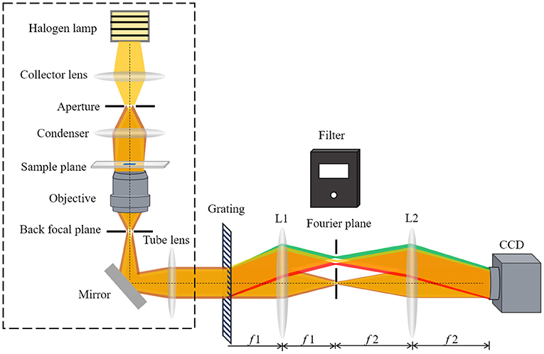
Figure 1. The wDPM add-on module uses a 4-f system coupled to the output port of a bright light microscope. A camera is placed at the output of the module to record the interference intensity.

In wDPM system, the measured quantity is the temporal cross-correlation function of the object wave field and the reference wave field [21, 26, 29]. Because the two fields pass through the same optical components, the time delay between them is evaluated to zero, that is, τ = 0. Therefore, the measured quantity can be written as

\begin{array}{l} Γ_{s, r} (r, r, 0) = {〈 U_{s} (r, t) U_{r}^{*} (r, t) 〉}_{t} & (1) \end{array}

where U_s (r, t) is the object wave field, U_r (r, t) is the reference wave field, the angular bracket denotes ensemble average. Assuming that fields are ergodic and, thus, stationary. Thus, the ensemble averaging in Equation (1) can be replaced by time averaging. As a result of the generalized Wiener-Khintchine theorem, the cross-correlation function Γ_{s, r} (r, r, τ) is the Fourier transform of the cross-spectral density W_s,r (r, r, w). Thus, according to the central ordinate theorem, Equation (1) can be written as

\begin{array}{l} Γ_{s, r} (r, r, 0) = \int W_{s, r} (r, r, w) d w \\ = \int 〈 U_{s} (r, w) U_{r}^{*} (r, w) 〉 d w & (2) \end{array}

where U_s (r, w) and U $_{r}^{*}$ (r, w) are the Fourier transforms of U_s (r, t) and U $_{r}^{*}$ (r, t), respectively.

In order to establish the model of image formation, we further analyze the object and reference wave fields. The diffraction grating creates copies of the image at different angles, and the filter allows the 1st order to completely pass through the rectangular hole. Thus, the object light field at CCD plane can be written as U_s (r, w) = T(r)U_i (r, w), where U_i (r, w) is the illumination field at the sample plane and T(r) is the transmission function of the measured sample. However, the 0th order field is filtered by the pinhole, expressed as U_r (r, w) = [T(r)U_i (r, w)] ⊗ h₀(r), where h₀(r) is the Fourier transform of the transmission function of the 0th filter aperture, ⊗ denotes the two-dimensional convolution operator. Equation (1) can be written as

\begin{array}{l} Γ_{s, r} (r, r, 0) \\ = \int 〈 T (r) U_{i} (r, w) {[\int \int_{- \infty}^{\infty} T (r^{'}) U_{i} (r^{'}, w) h_{0} (r - r^{'}) d^{2} r^{'}]}^{*} 〉 d w \\ = T (r) \int [\int \int_{- \infty}^{\infty} W_{i} (r, r^{'}, w) h_{0}^{*} (r - r^{'}) T^{*} (r^{'}) d^{2} r^{'}] d w \\ = T (r) \int \int_{- \infty}^{\infty} Γ_{i} (r - r^{'}, 0) h_{0}^{*} (r - r^{'}) T^{*} (r^{'}) d^{2} r^{'} \\ = T (r) {[T (r) \otimes h (r)]}^{*} & (3) \end{array}

here, h(r) = $Γ_{i}^{*}$ (r, 0)h₀(r) where $Γ_{i}^{*}$ (r, 0) is the conjugated term of the temporal cross-correlation function of the illumination source, and Γ_i (r, 0) reflects the coherence of the illumination field; W_i (r, r′, w) is the cross-spectral density of the illumination field, assuming that fields are stationary, i.e., W_i(r, r′, w)=W_i(r–r′, w). Equation (3) establishes a relationship between the measured quantity Γ_{s, r} (r, r, 0) and the sample transmission function T(r). Solving the phase value from Equation (3), the relationship between the measured phase value and the true phase value can be obtained as:

\begin{array}{l} φ_{m} (r) = φ (r) - arg [(T \otimes h) (r)] & (4) \end{array}

here, ϕ_m(r) is the measured phase value, ϕ(r) is the true phase value, arg[(T ⊗ h)(r)] indicates that the measured phase distribution is smoothed. The effects of phase underestimation, can be clearly seen, that is, the measured phase value is lower than the true phase value, even causing a negative value around the edges of the object, which is known as the halo effect.

Conventionally, to obtain the true phase distribution, given correlation measurements of the light source Γ_i (r, 0) and the filter function h₀(r), Equation (4) is solved by the constrained optimization problem as follows

\begin{array}{l} φ^{†} (r) = \arg \min_{φ} {{‖ φ_{m} - φ (r) + \arg [e^{i φ (r)} \otimes_{r} (Γ_{i}^{*} h_{0}) (r)] ‖}_{2}^{2} \\ + λ T V (φ)} & (5) \end{array}

here, $T V = \int d^{2} r \sqrt{{(\partial φ / \partial x)}^{2} (r) + {(\partial φ / \partial y)}^{2} (r)}$ , is the total variation term, which suppresses the noise effects and enforces the sparsity assumption of the sample phase distribution. ||.||₂ denotes the l₂-norm. While successful for the phase values estimation, the approach suffers long computation times, impractical for real-time measurement [29].

The HFDNN Method

Here, we propose a deep learning approach that uses end-to-end learning to reconstruct the true phase from the measured phase. The end-to-end learning approach is to use a set of data, consisting of the measured phase images (ϕ_m)_n and their corresponding ground-truth phase images (ϕ(r))_n, where n = 1, …, N, to learn the parametric inverse mapping operator R(F) from the measured phase to the true phase. The inverse mapping operator R(F) can be expressed as:

\begin{array}{l} R (F) = arg {min}_{F} \sum_{n = 1}^{N} L ({(φ (r))}_{n}, F {{(φ_{m} (r))}_{n}}) + λ J (F) & (6) \end{array}

where F denotes the deep neural network model, which contains the two types of parameters. The first type includes the parameters that specify the structure of the network, such as the number of the layers and neurons in each layer, the size of the kernels, etc. This type of parameters needs to be determined before training according to the training data sets and the purpose of learning. The other type includes the internal weights of different convolutional kernels. The weight parameters are adjusted autonomously during the training. L is the loss function to calculate the error between (ϕ(r))_n and F{(ϕ_m)_n}. And J is a regularization function, aim of constraining iterations and avoiding overfitting, and λ is the coefficient for balancing the loss and the regularization. Once the inverse mapping has been learned autonomously, the neural network can be used to recover the true phase directly from the measured phase, removing the halo artifacts.

We propose a HFDNN model, which is plotted in Figure 2, partially inspired by the autoencoders [41], to realize halo-free white-light phase imaging. The HFDNN architecture is composed of the convolutional blocks, the pooling blocks, and the up-sampling blocks. The convolutional block is a convolutional layer, with an activation function, which is used to extract local features and increase the expression ability of measured data. The pooling block is a max pooling or an average pooling layer, which can selectively extract representative features and reduce parameters. The up-sampling block is an up-sampling layer used to restore high-dimensional features to the reconstructed data with the same size as the input data. There is an apostrophe in the middle of the HFDNN architecture, which means that the number of the blocks can be increased or decreased, according to the size and complexity of the data, which affects the feature representation of the data during the calculation process. It is worth noting that that the compression ratio of the pooling layer should be equal to the expansion ratio of the up-sampling layers, otherwise the data size will have a mismatch.

FIGURE 2

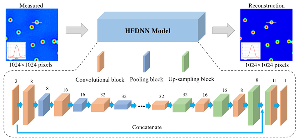
Figure 2. A schematic of the proposed HFDNN architecture. The digits above each layer denote the number of input channels.

In the proposed HFDNN architecture, the network first performs a 3 × 3 convolution operation with 3 channels to increase the depth on the input data. Then through three convolutional layers with 3 × 3 kernel size, whose channel numbers are 8, 16, and 32, respectively, to extract important local features, and each layer is interleaved with a 2 × 2 max pooling layer. By setting the down-sampling process as above, we can avoid extreme compression by increasing the number of channels of the feature map while reducing the size of the feature map. In the up-sampling process, there are also three 3 × 3 convolutional layers with 32,16 and 8 channels, respectively, and each layer is interleaved with a 2 × 2 up-sampling layer. And then we use the concatenation operation on the first convolutional layer and the last up-sampling layer to get a feature map of 11 channels. Each convolutional layer has rectified linear units (ReLU) [42], called an activation function, which allow for faster and more effective training of deep neural architectures on large and complex data sets. However, the final layer uses a depth-reducing 1 × 1 convolutional filter without an activation function to create the reconstructed data. In our network, the measured phase images with 1,024 × 1,024 pixels are used as the input to the HDFNN architecture. The image is calculated by the first 3 × 3 convolutional layer to increase the number of channels. After the following three convolutional and pooling calculations, the size of the data is reduced to 512 × 512 pixels, 256 × 256 pixels, 128 × 128 pixels, respectively, and the number of convolutional channels for extracting local features are 8, 16, and 32, respectively. During the up-sampling process, the data with 128 × 128 pixels is restored to the one with 1,024 × 1,024 pixels by symmetric three up-sampling calculations. Last, the halo-free phase image with the same size is outputted.

After the structure of the network is established, the network will be trained to obtain the internal weights. The process of training the HFDNN network is as shown in Figure 3. The input data is calculated by the HFDNN network to generate a reconstructed data every time. And the error is calculated by comparing the reconstructed data with the target data. We used the back-propagation algorithm to back propagate the error into the network, and the Adaptive Moment Estimation (Adam) [43] based optimization to optimize the weights. The weights at when the error remains a constant or reaches a value are saved. And the HFDNN network is established. In the method proposed in this paper, the error is calculated as

\begin{array}{l} e_{e r r o r} = \frac{1}{M \times N} {\sum_{u = 1}^{M} \sum_{v = 1}^{N} (F {{(φ_{m} (u, v))}_{n}} - φ {(u, v)}_{n})}^{2} & (7) \end{array}

where e_erroris the error between the reconstructed data and the target data.

FIGURE 3

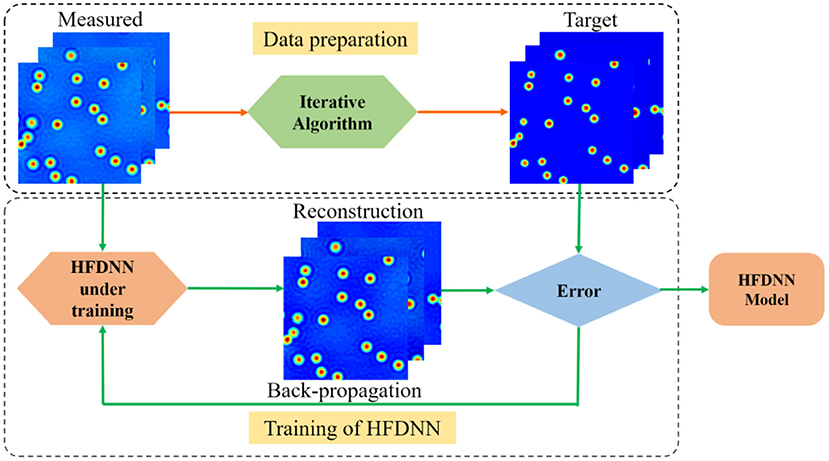
Figure 3. A schematic of the process of the HFDNN training. In the process of data preparation, the measured images are acquired by our wDPM system, which are used as the input data; the measured images are reversed into the halo-free images by the iterative algorithm, which are used as the target data. In the process of the HFDNN training, when the error remains a constant or reaches a value, the training is terminated and the HFDNN model is established.

The HFDNN architecture is implemented using Keras [44] with TensorFlow [45] backend. We perform the training and validation on a personal computer with two-core 2.60 GHz CPU, 56 GB of RAM, and Nvidia Quadro K5000. For the training of the model, we select an initial learning rate of 1e-4 for the Adam optimizer and train the network for 200 epochs on a batch of 8 training data with1,024 × 1,024 pixels.

Results and Discussion

Experimental Results

In order to verify the feasibility and accuracy of the proposed HFDNN approach, we carry out the experiments on our established wDPM system. In our initial set of experiments, we use 2 μm polystyrene beads as the samples. Its refractive index is 1.59. A small number of beads are taken and scattered on a slide, then the Olympus immersion oil (the refractive index is 1.518) is dropped to immerse the beads, finally the sample is covered with the cover glass. The prepared sample is placed on the stage of the microscope and imaged on the plane of the CCD camera. The interferograms at different field of view are captured. And the phase images are reconstructed by numerical computations. First, the complex amplitude of the object wave is obtained by the frequency domain filtering and inverse Fourier transform. Then, by phase unwrapping [46] and phase compensation operation by the method of the reference interferogram [47], the quantitative phase image is reconstructed. Due to the known refractive indexes and the center wavelength, the thickness image of the polystyrene beads can be further obtained from the reconstructed phase values by $h_{m} (x, y) = \frac{λ φ_{m} (x, y)}{2 π (n_{b e a d s} - n_{o i l})}$ .

For training the HFDNN network, 1000 interferograms with 1,024 × 1,024 pixels are captured at different fields of view for several samples on our experimental setup. After the reconstructing computation, these measured thickness images are used as the training data set. In order to augment the data set by four-fold, the measured data set are further augmented by rotating them to 0, 90, 180, and 270 deg. The true thickness images, used as the target data set, are recovered using the iterative deconvolution algorithm described in [29] based on the physical parameters of the image formation. As described in [29], the iterative method can successfully eliminate the halo effect to recover the true image. Therefore, the corresponding thickness images after the iterative calculations are taken as the target data set. For training the network, the data set is divided into the training and validation sets with the ratio of 7:3.

After the training, next we blindly test the HFDNN network on the samples that had no overlap with the training or validation sets. Figure 4 illustrates the success of HFDNN. Figure 4a is a measured thickness image of polystyrene beads. It is apparent that there are halo artifacts in the measured image, especially around the edges of the beads. Figure 4b is the thickness image calculated by the iterative algorithm in combination with the hardware parameters. It can be seen that the iterative calculation succeeded in eliminating the halo effect. Figure 4c is the thickness image calculated by the HFDNN. It clearly illustrates that our end-to-end deep learning method can eliminate halo artifacts like the iterative algorithm. In order to compare the performance with other previous methods, the reconstruction is also performed by the direct non-iterative algorithm based on Hilbert transform [26]. As shown in Figure 4d, the halo artifacts around the edges of the beads can be removed but the thickness of the beads is still underestimated than the ones in Figures 4b,c. Figure 4e is the line profiles along the same diameter of the same bead that further compares the measured data, the target data, the reconstructed data calculated by the HFDNN and by the direct non-iterative algorithm, respectively. Through the comparison of the line profiles, it is more clearly seen that the reconstructed data by the HFDNN is almost identical with the target data but the one by the non-iterative algorithm seems like a non-negative clipping. Therefore, Figure 4 illustrates that the HFDNN can successfully correct halo effect, that is, the negative values surrounding the beads in the measured data is removed and the thickness of the reconstructed beads converges to our expected value of 2 μm. The HFDNN algorithm is written in Python and optimized by GPU codes. Using the HFDNN, it takes only about 60 ms to achieve a halo-free image reconstruction on our personal computer, which is much more efficient than using the iterative algorithm (also written in Python and optimized by GPU codes), which takes about 600 ms for the same image. Although the non-iterative algorithm can reconstruct an image a little faster than the HFDNN, it can only remove the negative values around the edge of the object but not correct the underestimated values to the accurate measurement.

FIGURE 4

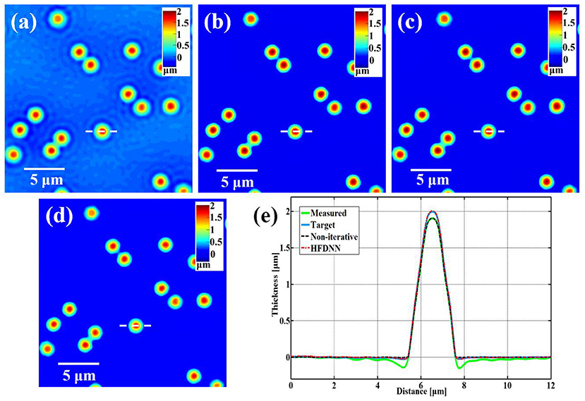
Figure 4. The reconstructed results of standard polystyrene beads. (a) The measured image; (b) the target data; (c) the reconstructed image by our HFDNN; (d) the reconstructed image by the non-iteratitave method —“Non-iterative” in [26]; (e) the thickness profiles along the same diameter of the same bead drawn in (a–d); the green curve illustrates the profile of the measured data; the blue curve illustrates the profile of the target data; the red dash curve illustrates the profile of the HFDNN output data; the black dash curve illustrates the profile of the non-iterative reconstruction.

Based on the argument of deep learning, the HFDNN approach should let the network learn halo-effect features by the training, i.e., the deep learning method should be generalized for different types of samples. In order to test this generalization, next we test the HFDNN on the measured phase data of living red blood cells captured by our wDPM system. Still using the HFDNN architecture as shown in Figure 2, only the training data set is changed. The red blood cells are obtained from our local hospital using venipuncture and stored in a refrigerator at 4°C. The blood is diluted to a concentration of 0.2% in PBSA solution (0.5% Bovine Serum Albumin in PBS). To prevent cell tilt during imaging, a sample chamber is prepared by punching a hole into a piece of double-sided scotch tape and sticking the tape onto a coverslip. After dispensing a drop of blood into this circular chamber, the drop is sealed from the top by a Poly-L-lysine coated coverslip. The coverslip pair is then turned over and the cells are allowed to settle for 1 h before imaging so that they become immobilized. The prepared samples are placed on the objective stage and focused onto the CCD camera. Also for training the network, we capture 800 interferograms at different fields of view for several samples. The phase image is reconstructed as shown in Figure 5a, which is severely affected by halo artifacts. Then by the iterative calculation, halo-free phase images are obtained as shown in Figure 5b, used as the target data. And the data set is still augmented by four-fold. The data set is still divided into the training and validation sets with the ratio of 7:3. After the training, the weights of the network are iteratively updated. We blindly test the HFDNN network on the samples that had no overlap with the training or validation sets. The result is shown in Figure 5c. It can be seen from the visualization that halo artifacts are successfully corrected. For comparing, we also reconstruct the image by the non-iterative algorithm. As shown in Figure 5d, the halo artifacts around the edges of the cells can be removed but the phase values are still underestimated. Through the further comparison of the line profiles in Figure 5e, the reconstructed data by the HFDNN is almost identical with the target data by the iterative calculation and the one by the non-iterative algorithm seems like only a negative removing. The results illustrate that the HFDNN model can successfully remove the halo artifacts for other sample types.

FIGURE 5

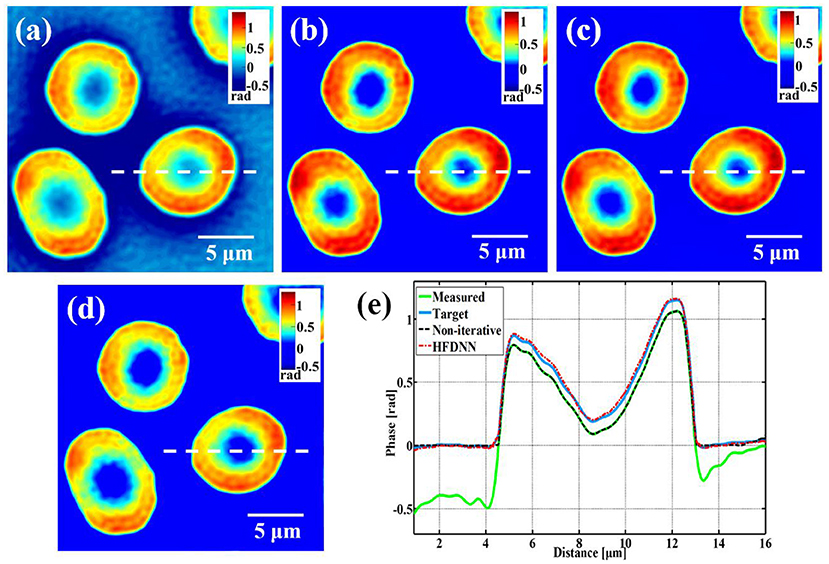
Figure 5. The reconstructed results of living red blood cells. (a) The measured image; (b) the target data; (c) the reconstructed image by the HFDNN; (d) the reconstructed image by the non-iteratitave method; (e) the phase profiles along the same position of the same cell drawn in (a–d); the green curve illustrates the profile of the measured data; the blue curve illustrates the profile of the target data; the red dash curve illustrates the profile of the HFDNN output data; the black dash curve illustrates the profile of the non-interative reconstruction.

Discussion

First, to further quantify the accuracy of our proposed HFDNN method, two evaluation metrics are used to evaluate our reconstructed data. One is the normalized root of mean square error (NRMSE) as follows:

\begin{array}{l} N R M S E = \sqrt{\frac{\frac{1}{M \times N} \sum_{u = 1}^{M} \sum_{v = 1}^{N} {(\tilde{φ} (u, v) - φ (u, v))}^{2}}{\frac{1}{M \times N} \sum_{u = 1}^{M} \sum_{v = 1}^{N} φ {(u, v)}^{2}}} & (8) \end{array}

where φ (u, v) is the target data, and $\tilde{φ}$ (u, v) is the reconstructed data by HFDNN. The smaller the NRMSE, the closer the reconstructed data is to the target data.

The second one is the Structural Similarity Index (SSIM) as follows:

\begin{array}{l} S S I M = \frac{(2 μ_{φ} μ_{\tilde{φ}} + c_{1}) (2 σ_{φ, \tilde{φ}} + c_{2})}{(μ_{φ}^{2} + μ_{\tilde{φ}}^{2} + c_{1}) (σ_{φ}^{2} + σ_{\tilde{φ}}^{2} + c_{2})} & (9) \end{array}

where φ and $\tilde{φ}$ represent the target data and the reconstructed data, respectively, μ is the mean of the data, σ² is the variance of the data, and $σ_{φ, \tilde{φ}}$ is the covariance of the two data, c₁ and c₂ are two constants. The range of SSIM is from 0 to 1, and when the reconstructed data is the same as the target data, the SSIM takes a value of 1.

We calculate the NRMSE and the SSIM over the test images as the metric values. For the polystyrene beads, the NRMES and the SSIM are 0.025 and 0.980, respectively. For the red blood cells, the NRMES and the SSIM are 0.073 and 0.941, respectively. For comparing, the NRMSE and the SSIM are also calculated over the reconstructed images by the direct non-iterative method. For the polystyrene beads, the NRMES and the SSIM are 0.085 and 0.863, respectively. For the red blood cells, the NRMES and the SSIM are 0.162 and 0.814, respectively. It can be seen from the two image metric values that the proposed HFDNN can more accurately correct the halo artifacts than the direct non-iterative method.

Second, the generalization of the HFDNN will be further discussed. Although in the experiments of red blood cells, the reconstructed results are calculated by the re-trained HFDNN network. Factually, as shown in Figure 6 there are almost no differences between the reconstructed results by the re-trained network and by the network without being re-trained. For further comparison, we also analyze the NRMES and the SSIM between the reconstructed results and the target data. Using the network without being re-trained, the NRMES and the SSIM are 0.094 and 0.923, respectively. And using the re-trained network, the NRMES and the SSIM are 0.073 and 0.941, respectively. However, the NRMES and the SSIM between the measured results and the target data are 0.514 and 0.665, respectively. It is clear that using the HFDNN network without being re-trained also can reconstruct high-quality images on red blood cells. Therefore, re-training the network, when a new type of samples is introduced, should be emphasized as a guarantee of the best results. In order to further prove the generalization of the HFDNN, we also applied it to other sample types which are morphologically different. The spores in monascus are imaged by our wDPM system. A small number of spores are diluted in water and dropped into a sample chamber, which is prepared by punching a hole into a piece of double-sided scotch tape and sticking the tape onto a coverslip. After dispensing a drop of the spores into this circular chamber, the drop is sealed from the top by a coverslip. The sample is stored under the room temperature of 25 °C. After about 1 day, the spores grow out the hyphae branches. Figure 7 is the reconstructed results for the spores and Figure 8 is the reconstructed results for the hyphae branches. It can be seen from the visualization that halo artifacts are successfully corrected. The results show that the HFDNN approach is generalized to different sample types.

FIGURE 6

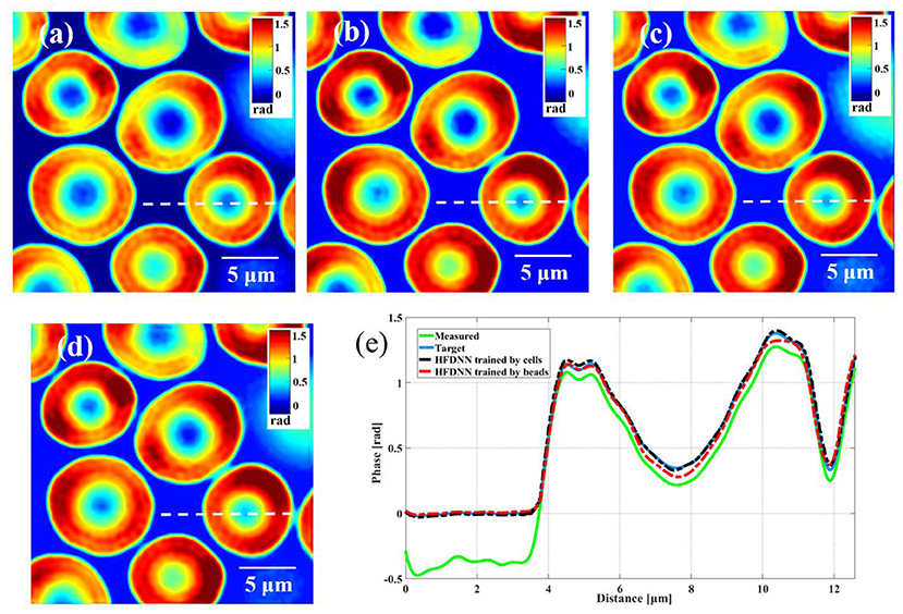
Figure 6. The comparison of the reconstructed results of living red blood cells. (a) The measured image; (b) the target data by the iteration method; (c) the reconstructed image by the HFDNN trained by red blood cells; (d) the reconstructed image by the HFDNN trained by beads; (e) the phase profiles along the same position of the same cell drawn in (a–d); the green curve illustrates the profile of the measured data; the blue curve illustrates the profile of the target data; the black dash curve illustrates the profile of the HFDNN trained by cells; the red dash curve illustrates the profile of the HFDNN trained by beads.

FIGURE 7

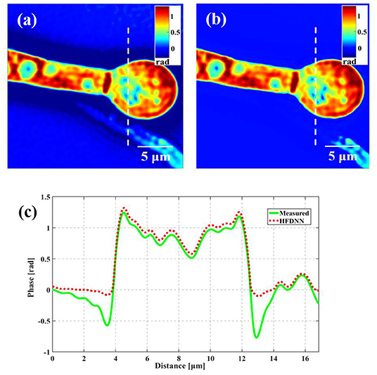
Figure 7. The reconstructed results of the spores in monascus. (a) The measured image; (b) the reconstructed image by the HFDNN without re-training; (c) the phase profiles along the same position drawn in (a,b); the green curve illustrates the profile of the measured data; the red dash curve illustrates the profile of the HFDNN.

FIGURE 8

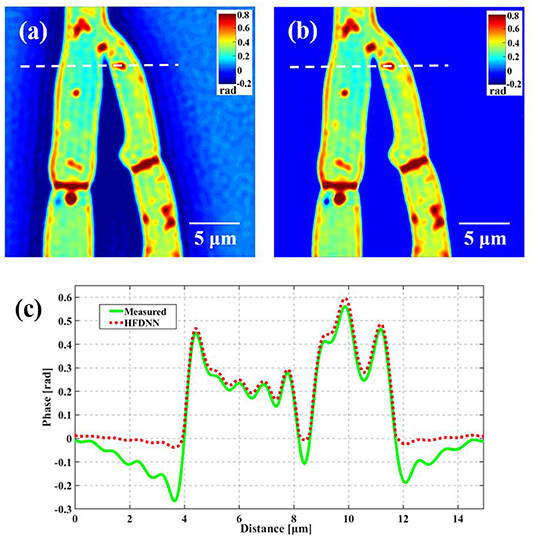
Figure 8. The reconstructed results of the hyphae branches in monascus. (a) The measured image; (b) the reconstructed image by the HFDNN without re-training; (c) the phase profiles along the same position drawn in (a,b); the green curve illustrates the profile of the measured data; the red dash curve illustrates the profile of the HFDNN.

On the other hand, the HFDNN method does not rely on any system parameter, which lets the network learn the features of halo artifacts by the training. There exists the low spatiotemporal noise in wDPM due to its common-path, white-light illumination approach. When the systems are well-established, although in different measurements on the same system or on different systems there are minor differences to some extent between system SNR, alignment, etc., the features of halo artifacts for the same type of samples will be the same. Therefore, it is not necessary to re-train the network when measuring the same type of samples at different measurements on the same microscope or even on different microscopes.

At last, it should be pointed out that the mass measurements are often required for some types of samples in the practical applications. Therefore, even if we have to collect training data (both with halo and halo-free phase images) on that specific type of cells and redo the training process, we still can get the more benefits because the deep-learning-based method can rapidly and accurately remove the halo artifacts in the following mass measurements.

Conclusions

In summary, we present the HFDNN method, a deep-learning-based approach for halo-free white-light phase diffraction imaging. Unlike the conventional iterative approach, the proposed deep convolutional neural network can be applied to the high-speed elimination of halo effects on various samples. The feasibility of the method is illustrated by the experimental data captured on our wDPM setup. Factually, the HFDNN method provides new avenues in all white-light phase imaging field. The HFDNN can learn the features that the phase images possess due to the halo effects. Thus, it can eliminate halo artifacts for different samples in various white-light phase images. In the future, we aim to validate our algorithm on a larger dataset on more types of objects to make our algorithm more robust to sample variation and to improve the generilizeation.

Data Availability Statement

The raw data supporting the conclusions of this article will be made available by the authors, without undue reservation.

Author Contributions

KZ and LM conceived the idea of the HFDNN method. KZ and MZ were involved in the design and construction the HFDNN network. MZ and LM analyzed the data. JZ gathered the experimental data. LM, MZ, and YL wrote the paper. All authors contributed to the article and approved the submitted version.

Funding

The Natural Science Foundation of Zhejiang Provincial of China (Grant No. LY17F050002); the National Natural Science Foundation of China (Grant No. 61205012).

Conflict of Interest

The authors declare that the research was conducted in the absence of any commercial or financial relationships that could be construed as a potential conflict of interest.

References

1. Popescu G. Quantitative Phase Imaging of Cells and Tissues. New York, NY: McGraw-Hill (2011).

PubMed Abstract | Google Scholar

2. Barer R. Determination of dry mass, thickness, solid and water concentration in living cells. Nature. (1953) 172:1097–8. doi: 10.1038/1721097a0

PubMed Abstract | CrossRef Full Text | Google Scholar

3. Uttam S, Pham HV, LaFace J, Leibowitz B, Yu J, Brand RE, et al. Early prediction of cancer progression by depth-resolved nanoscale mapping of nuclear architecture from unstained tissue specimens. Cancer Res. (2015) 75:4718–27. doi: 10.1158/0008-5472.CAN-15-1274

PubMed Abstract | CrossRef Full Text | Google Scholar

4. Ma L, Rajshekhar G, Wang R, Bhaduri B, Sridharan S, Mir M, et al. Phase correlation imaging of unlabeled cell dynamics. Sci Rep. (2016) 6:32702. doi: 10.1038/srep32702

PubMed Abstract | CrossRef Full Text | Google Scholar

5. Huang D, Swanson EA, Lin CP, Schuman JS, Stinson WG, Chang W, et al. Optical coherence tomography. Science. (1991) 254:1178–81. doi: 10.1126/science.1957169

CrossRef Full Text | Google Scholar

6. Izatt JA, Boppart S, Bouma B, Boer JD, Drexler W, Li X, et al. Introduction to the feature issue on the 25 year anniversary of optical coherence tomography. Biomed Opt Expr. (2017) 8:3289–91. doi: 10.1364/BOE.8.003289

PubMed Abstract | CrossRef Full Text | Google Scholar

7. Cuche E, Bevilacqua F, Depeursinge C. Digital holography for quantitative phase-contrast imaging. Opt Lett. (1999) 24:291–3. doi: 10.1364/OL.24.000291

PubMed Abstract | CrossRef Full Text | Google Scholar

8. Colomb T, Cuche E, Charrière F, Kühn J, Aspert N, Montfort F, et al. Automatic procedure for aberration compensation in digital holographic microscopy and applications to specimen shape compensation. Appl Opt. (2006) 45:851–63. doi: 10.1364/AO.45.000851

PubMed Abstract | CrossRef Full Text | Google Scholar

9. Popescu G, Ikeda T, Dasari RR, Feld MS. Diffraction phase microscopy for quantifying cell structure and dynamics. Opt Lett. (2006) 31:775–7. doi: 10.1364/OL.31.000775

PubMed Abstract | CrossRef Full Text | Google Scholar

10. Majeed H, Ma L, Lee YJ, Kandel M, Min E, Jung W, et al. Magnified image spatial spectrum (MISS) microscopy for nanometer and millisecond scale label-free imaging. Opt Expr. (2018) 26:5423–40. doi: 10.1364/OE.26.005423

PubMed Abstract | CrossRef Full Text | Google Scholar

11. Teague MR. Deterministic phase retrieval: a green's function solution. J Opt Soc Am. (1983) 73:1434–41. doi: 10.1364/JOSA.73.001434

CrossRef Full Text | Google Scholar

12. Zuo C, Sun J, Li J, Zhang J, Asundi A, Chen Q. High-resolution transport-of-intensity quantitative phase microscopy with annular illumination. Sci Rep. (2017) 7:7654. doi: 10.1038/s41598-017-06837-1

PubMed Abstract | CrossRef Full Text | Google Scholar

13. Wolf E. Three-dimensional structure determination of semi-transparent objects from holographic data. Opt Commun. (1969) 1:153–6. doi: 10.1016/0030-4018(69)90052-2

CrossRef Full Text | Google Scholar

14. Su L, Ma L, Wang H. Improved regularization reconstruction from sparse angle data in optical diffraction tomography. Appl Opt. (2015) 54:859–68. doi: 10.1364/AO.54.000859

PubMed Abstract | CrossRef Full Text | Google Scholar

15. Zheng C, Zhou R, Kuang C, Zhao G, Yaqoob Z, So PTC. Digital micromirror device-based common-path quantitative phase imaging. Opt Lett. (2017) 42:1448–51. doi: 10.1364/OL.42.001448

PubMed Abstract | CrossRef Full Text | Google Scholar

16. Schnars U, Jüptner W. Direct recording of holograms by a CCD target and numerical reconstruction. Appl Opt. (1994) 33:179–81. doi: 10.1364/AO.33.000179

PubMed Abstract | CrossRef Full Text | Google Scholar

17. Bhaduri B, Pham H, Mir M, Popescu G. Diffraction phase microscopy with white light. Opt Lett. (2012) 37:1094–6. doi: 10.1364/OL.37.001094

CrossRef Full Text | Google Scholar

18. Shan M, Kandel ME, Majeed H, Nastasa V, Popescu G. White-light diffraction phase microscopy at doubled space-bandwidth product. Opt Expr. (2016) 24:29033–9. doi: 10.1364/OE.24.029033

PubMed Abstract | CrossRef Full Text | Google Scholar

19. Kemper B, Stürwald S, Remmersmann C, Langehanenberg P, von Bally G. Characterisation of light emitting diodes (LEDs) for application in digital holographic microscopy for inspection of micro and nanostructured surfaces. Opt Lasers Eng. (2008) 46:499–507. doi: 10.1016/j.optlaseng.2008.03.007

CrossRef Full Text | Google Scholar

20. Farrokhi H, Boonruangkan J, Chun BJ, Rohith TM, Mishra A, Toh HT, et al. Speckle reduction in quantitative phase imaging by generating spatially incoherent laser field at electroactive optical diffusers. Opt Expr. (2017) 25:10791–800. doi: 10.1364/OE.25.010791

PubMed Abstract | CrossRef Full Text | Google Scholar

21. Nguyen TH, Edwards C, Goddard LL, Popescu G. Quantitative phase imaging with partially coherent illumination. Opt Lett. (2014) 39:5511–4. doi: 10.1364/OL.39.005511

PubMed Abstract | CrossRef Full Text | Google Scholar

22. Maurer C, Jesacher A, Bernet S, Ritsch-Marte M. Phase contrast microscopy with full numerical aperture illumination. Opt Expr. (2008) 16:19821–9. doi: 10.1364/OE.16.019821

PubMed Abstract | CrossRef Full Text | Google Scholar

23. Edwards C, Nguyen TH, Popescu G, Goddard LL. Image formation and halo removal in diffraction phase microscopy with partially coherent illumination. In: Frontiers in Optics 2014. Tucson, AZ (2014). doi: 10.1364/FIO.2014.FTu4C.5

CrossRef Full Text | Google Scholar

24. Otaki T. Artifact halo reduction in phase contrast microscopy using apodization. Opt Rev. (2000) 7:119–22. doi: 10.1007/s10043-000-0119-5

CrossRef Full Text | Google Scholar

25. Edwards C, Bhaduri B, Nguyen T, Griffin BG, Pham H, Kim T, et al. Effects of spatial coherence in diffraction phase microscopy. Opt Expr. (2014) 22:5133–46. doi: 10.1364/OE.22.005133

PubMed Abstract | CrossRef Full Text | Google Scholar

26. Kandel ME, Fanous M, Best-Popescu C, Popescu G. Real-time halo correction in phase contrast imaging. Biomed Opt Expr. (2018) 9:623–35. doi: 10.1364/BOE.9.000623

PubMed Abstract | CrossRef Full Text | Google Scholar

27. Yin Z, Kanade T, Chen M. Understanding the phase contrast optics to restore artifact-free microscopy images for segmentation. Med Image Anal. (2012) 16:1047–62. doi: 10.1016/j.media.2011.12.006

PubMed Abstract | CrossRef Full Text | Google Scholar

28. Jaccard N, Griffin LD, Keser A, Macown RJ, Super A, Veraitch FS, et al. Automated method for the rapid and precise estimation of adherent cell culture characteristics from phase contrast microscopy images. Biotechnol Bioeng. (2014) 111:504–17. doi: 10.1002/bit.25115

PubMed Abstract | CrossRef Full Text | Google Scholar

29. Nguyen TH, Kandel M, Shakir HM, Best-Popescu C, Arikkath J, Do MN, et al. Halo-free phase contrast microscopy. Sci Rep. (2017) 7:44034. doi: 10.1038/srep44034

PubMed Abstract | CrossRef Full Text | Google Scholar

30. Lecun Y, Bengio Y, Hinton G. Deep learning. Nature. (2015) 521:436–44. doi: 10.1038/nature14539

CrossRef Full Text | Google Scholar

31. Schmidhuber J. Deep learning in neural networks: an overview. Neural Netw. (2015) 61:85–117. doi: 10.1016/j.neunet.2014.09.003

PubMed Abstract | CrossRef Full Text | Google Scholar

32. Horisaki R, Takagi R, Tanida J. Learning-based imaging through scattering media. Opt Expr. (2016) 24:13738–43. doi: 10.1364/OE.24.013738

CrossRef Full Text | Google Scholar

33. Li S, Deng M, Lee J, Sinha A, Barbastathis G. Imaging through glass diffusers using densely connected convolutional networks. Optica. (2018) 5:803–13. doi: 10.1364/OPTICA.5.000803

CrossRef Full Text | Google Scholar

34. Lyu M, Wang W, Wang H, Wang H, Li G, Chen N, et al. Deep-learning-based ghost imaging. Sci Rep. (2017) 7:17865. doi: 10.1038/s41598-017-18171-7

CrossRef Full Text | Google Scholar

35. Cheng YF, Strachan M, Weiss Z, Deb M, Carone D, Ganapati V. Illumination pattern design with deep learning for single-shot Fourier ptychographic microscopy. Opt Expr. (2019) 27:644–56. doi: 10.1364/OE.27.000644

PubMed Abstract | CrossRef Full Text | Google Scholar

36. Rivenson Y, Zhang Y, Günaydin H, Teng D, Ozcan A. Phase recovery and holographic image reconstruction using deep learning in neural networks. Light Sci Appl. (2018) 7:17141. doi: 10.1038/lsa.2017.141

PubMed Abstract | CrossRef Full Text | Google Scholar

37. Wu Y, Rivenson Y, Zhang Y, Wei Z, Günaydin H, Lin X, et al. Extended depth-of-field in holographic imaging using deep-learning-based autofocusing and phase recovery. Optica. (2018) 5:704–10. doi: 10.1364/OPTICA.5.000704

CrossRef Full Text | Google Scholar

38. Wang P, Di J. Deep learning-based object classification through multimode fiber via a CNN-architecture SpeckleNet. Appl Opt. (2018) 57:8258–63. doi: 10.1364/AO.57.008258

PubMed Abstract | CrossRef Full Text | Google Scholar

39. Nguyen TH, Sridharan S, Macias V, Kajdacsy-Balla A, Melamed J, Do MN, et al. Automatic Gleason grading of prostate cancer using quantitative phase imaging and machine learning. J Biomed Opt. (2017) 22:036015. doi: 10.1117/1.JBO.22.3.036015

PubMed Abstract | CrossRef Full Text | Google Scholar

40. Feng S, Chen Q, Gu G, Tao T, Zhang L, Hu Y, et al. Fringe pattern analysis using deep learning. Adv Photonics. (2019) 1:025001. doi: 10.1117/1.AP.1.2.025001

CrossRef Full Text | Google Scholar

41. Hinton GE, Salakhutdinov RR. Reducing the dimensionality of data with neural networks. Science. (2006) 313:504–7. doi: 10.1126/science.1127647

PubMed Abstract | CrossRef Full Text | Google Scholar

42. Petersen P, Voigtlaender F. Optimal approximation of piecewise smooth functions using deep ReLU neural networks. Neural Netw. (2018) 108:296–330. doi: 10.1016/j.neunet.2018.08.019

PubMed Abstract | CrossRef Full Text | Google Scholar

43. Kingma DP, Ba J. Adam: a method for stochastic optimization. arXiv. (2017) arXiv:1412.6980.

Google Scholar

44. Chollet F. Keras. Available online at:https://github.com/keras-team/keras

Google Scholar

45. Abadi M, Agarwal A, Barham P, Brevdo E, Chen J, Chen Z, et al. Tensorflow: Large-scale machine learning on heterogeneous distributed systems. arXiv [Preprint].

Google Scholar

46. Ma L, Li Y, Wang H, Jin H. Fast algorithm for reliability-guided phase unwrapping in digital holographic microscopy. Appl Opt. (2012) 51:8800–7. doi: 10.1364/AO.51.008800

PubMed Abstract | CrossRef Full Text | Google Scholar

47. Ferraro P, De Nicola S, Finizio A, Coppola G, Grilli S, Magro C, et al. Compensation of the inherent wave front curvature in digital holographic coherent microscopy for quantitative phase-contrast imaging. Appl Opt. (2003) 42:1938–46. doi: 10.1364/AO.42.001938

PubMed Abstract | CrossRef Full Text | Google Scholar

Keywords: quantitative phase imaging, diffraction phase microscopy, deep learning, halo-free, white-light illumination

Citation: Zhang K, Zhu M, Ma L, Zhang J and Li Y (2021) Deep-Learning-Based Halo-Free White-Light Diffraction Phase Imaging. Front. Phys. 9:650108. doi: 10.3389/fphy.2021.650108

Received: 06 January 2021; Accepted: 16 March 2021;
Published: 12 April 2021.

Edited by:

Chao Zuo, Nanjing University of Science and Technology, China

Reviewed by:

Jiaji Li, Nanjing University of Science and Technology, China
Zahid Yaqoob, Massachusetts Institute of Technology, United States

Copyright © 2021 Zhang, Zhu, Ma, Zhang and Li. This is an open-access article distributed under the terms of the Creative Commons Attribution License (CC BY). The use, distribution or reproduction in other forums is permitted, provided the original author(s) and the copyright owner(s) are credited and that the original publication in this journal is cited, in accordance with accepted academic practice. No use, distribution or reproduction is permitted which does not comply with these terms.

*Correspondence: Lihong Ma, zjnumlh@zjnu.cn

ORIGINAL RESEARCH article

Deep-Learning-Based Halo-Free White-Light Diffraction Phase Imaging

Introduction

Experimental Setup

The HFDNN Method

Results and Discussion

Experimental Results

Discussion

Conclusions

Data Availability Statement

Author Contributions

Funding

Conflict of Interest

References

This article is part of the Research Topic

People also looked at