 Sepehr Sima
 Mehdi Sanayei
- School of Cognitive Sciences, Institute for Research in Fundamental Sciences (IPM), Tehran, Iran
Time and space are two intertwined contexts that frame our cognition of the world and have shared mechanisms. A well-known theory on this case is “A Theory of Magnitude (ATOM)” which states that the perception of these two domains shares common mechanisms. However, evidence regarding shared computations of time and space is intermixed. To investigate this issue, we asked human subjects to reproduce time and distance intervals with saccadic eye movements in similarly designed tasks. We applied an observer model to both modalities and found underlying differences in the processing of time and space. While time and space computations are both probabilistic, adding priors to space perception minimally improved model performance, as opposed to time perception which was consistently better explained by Bayesian computations. We also showed that while both measurement and motor variability were smaller in distance than time reproduction, only the motor variability was correlated between them, as both tasks used saccadic eye movements for response. Our results suggest that time and space perception abide by the same algorithm but have different computational properties.
1 Introduction
The study of time perception has demonstrated the complex interplay of spatiotemporal information in the brain. As temporal processes are linked to their embodied experience of the environment (Safaie et al., 2020), analyzing the spatial dimension in the study of time perception can provide a powerful tool for understanding the underlying mechanisms that allow us to comprehend the external world. Time and space are two aspects of the physical world that frame our experience of the world. The perception of time and space occurs in an interrelated fashion in human cognition, and recent research shows a growing interest in understanding the underlying mechanisms of their relationship (Goldreich, 2007; Robinson and Wiener, 2021; Schroeger et al., 2022; Whitaker et al., 2022). It has been suggested that time perception occurs through spatialization of time intervals in the face of movement-based events of the world (Robbe, 2023). Such spatialization could be seen in the way we have tied the perception of time to space by devising various types of clocks to keep track of the passage of time.
In modern science, time and space have been represented with measurable proxies imbued with operational definitions, i.e., time and distance intervals, respectively (Buzsáki and Llinás, 2017), which provide a framework for studying and quantifying these abstract concepts. This has made possible the study of the relationship between time and space perception. A variety of time-space interactions in the human perceptual system has been observed. For example, spatiotemporal interference is one such interaction where spatial information can distort the perception of temporal information and vice versa (Vidaud-Laperrière et al., 2022). Peri-saccadic spatiotemporal compression is another phenomenon that serves as evidence of common mechanisms in the perception of time and space (Morrone et al., 2005).
A Theory of Magnitude (ATOM) proposed by Walsh (2003) suggests that the brain has a core common magnitude system for time, space, and quantity. According to this theory, the neural mechanisms underlying the perception of time, space, and quantity are intertwined, and the brain processes these dimensions in a unified manner. This theory has been supported by empirical evidence from studies that have shown that the perception of time and space share common neural substrates (Casasanto and Boroditsky, 2008; Howard et al., 2014; Cai and Connell, 2016; Chen et al., 2021; Cui et al., 2022; Jie and Youguo, 2023). A recent meta-analysis of neuroimaging studies (Cona et al., 2021) has suggested that there is a common system of brain regions that are activated during both time and space processing, including bilateral insula, the pre-supplementary motor area (pre-SMA), the right frontal operculum, and intraparietal sulci. At the neuronal level, it has been observed that spatial information could at least be partially derived from temporal information (Burgess et al., 2011).
Despite these findings, the precise nature and the extent to which these perceptual domains share common mechanisms remain unknown. This has spurred several investigations into better understanding the relationship between time and space (Abramson et al., 2023; Schonhaut et al., 2023). Most studies to date have approached the question in terms of the interferences that occur between perceptual domains (Marcos and Genovesio, 2017; Martin et al., 2017; Üstün et al., 2022). We attempted to approach this question by utilizing behavioral modeling and model comparison.
A Bayesian understanding of timing has revealed that the interaction of the temporal context and the internal ongoing processes culminates in the calibration of estimated intervals (Sadibolova and Terhune, 2022) in the form of perceptual biases. Such a formulation of interval timing presents us with two stages in the process of timing, i.e., the measurement (perception) and the reproduction (action) phases of interval timing (Jazayeri and Shadlen, 2010). The link between the measurement and the reproduction is actualized by an estimation function in the observer model. Based on the nature of the observer model (ideal vs. non-ideal), the estimation functions differ. Bayesian least squares (BLS) and maximum likelihood estimation (MLE) estimators have been used in the literature as prior-dependent and prior-independent functions, respectively (Jazayeri and Shadlen, 2010). The Bayesian perspective has also been explored in human spatial navigation (Petzschner and Glasauer, 2011; Thurley and Schild, 2018). Thus, the probabilistic nature of spatiotemporal information could be well captured by an optimum-seeking system which combines experience-dependent information with contextual noisy measurements to generate an estimate of various facets of time and space. It remains unclear whether the perceptual biases in time and space are both attributable to the prior information.
In this study, we compared how spatial and temporal measurements are implemented by probing sources of variability in the process of time and distance measurement and reproduction, within a probabilistic framework. We used saccadic eye movement as the effector to reproduce presented time/distance intervals. In each block, the subjects had to reproduce the presented time/distance interval by making a saccade to a predefined target in case of time reproduction or to a point on a predefined line to reproduce the presented distance. We showed that the perceptual biases in time perception are explained by prior-dependent computations, as previously shown in the literature. On the other hand, we cast doubt on the contribution of prior information to the observed perceptual biases in space perception.
2 Materials and methods
2.1 Apparatus
The experiments were carried out on a computer running Linux operating system, on MATLAB (2016b), with Psychtoolbox 3 extension (Brainard, 1997). Stimuli were presented on a monitor (17″) placed ∼60 cm from the subject with a 60 Hz refresh rate. The subject sat comfortably on a chair in a dimly lit room to participate in this study, with the head stabilized by a head and chin rest. An EyeLink 1000 infrared eye tracking system (SR Research, Mississauga, Ontario) was used to record eye movements at 1 kHz.
2.2 Subjects
We enrolled 22 volunteers (12 female, range: [20, 43], mean ± SD: 26.5 ± 5.5). All were naïve to the purpose of the study except 2 (subjects 1 and 2) who were the authors of this study. We excluded 1 subject because of the troubled eye-tracker calibration caused by her contact lens and 1 subject because of excessively large eye-calibration errors. All subjects had normal or correct-to-normal vision. They had signed the consent form prior to the experiment. The experiment was approved by the ethics committee of the School of Cognitive Sciences (IPM). We counter-balanced all variables and blocks between participants. Half of the participants completed the time reproduction task first. Before starting each experiment, each participant completed a full block of training to familiarize themselves with each task.
2.3 Experiment 1
We designed a time reproduction task in which subjects had to reproduce perceived time intervals. At the beginning of each block, the name of the condition (time) was displayed at the center of the screen. The participant then pressed the space bar to start the block. A white fixation cross with a length of 0.5° was presented at the center of the screen for 1 s. After participants acquired fixation, a black line was then presented for a variable duration of 500–1,000 ms (uniform distribution). The participants were instructed to keep their gaze on the fixation point (within a 4° × 4° window). The line extended from the fixation cross to one of the four corners of the screen. The location of the line was fixed within each block, but changed between blocks. After that, a white circle (“set,” diameter of 1.5°) was flashed on the horizontal meridian, contra-lateral to the black line. The eccentricity of the circle was 6, 8, or 12°, randomly chosen on each trial. After a variable sample interval of 0.4, 0.8, or 1.6 s, a white circle (“go,” diameter of 1.5°) was presented on the black line at the same eccentricity as the flashed circle. Participants were then required to reproduce the duration between the onset of the “set” stimulus and the onset of the “go” stimulus by making a saccade to the “go” target to reproduce the sample interval. The initiation of the saccade was defined as the time the eye exited the fixation window (4° × 4°). If the saccade was landed within a 4° × 4° window of the “go” stimulus within 100 ms of the saccade initiation and stayed in the window for 100 ms, the go stimulus would turn to green (Figure 1A). The reproduced time was calculated as the interval between the “go” presentation and the initiation of the saccade. We did not provide any feedback regarding the accuracy of the timing. Each block consisted of 54 trials (3 eccentricities, 3 sample interval, and 6 repetitions for each condition) and subjects performed 8 blocks.
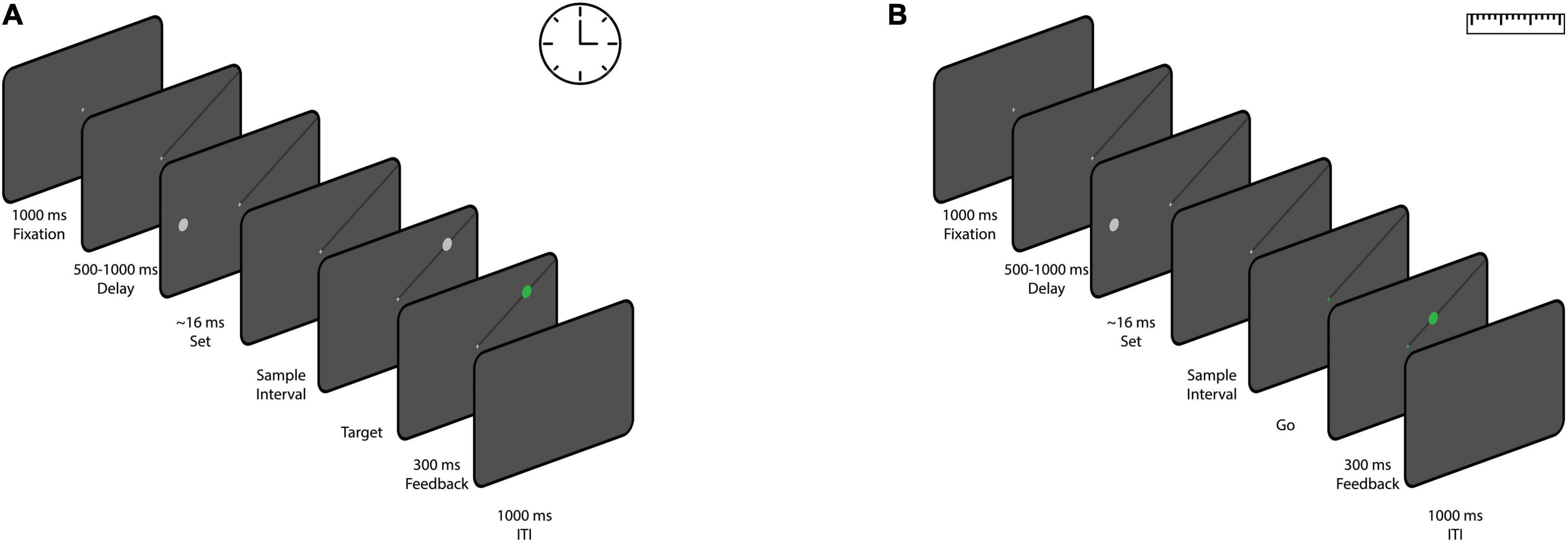
Figure 1. The sequence of trial events for the time reproduction task (A) and the distance reproduction task (B). (A) Participants were given a time reproduction task in which they had to reproduce sample time intervals. After acquiring fixation and the presentation of a black line on screen, A white circle (“set”) appeared on the horizontal meridian of the screen, and after a sample interval, another white circle (“go”) appeared on the black line. Participants had to reproduce the sample interval by making a saccade to the “go” stimulus. Successful saccades turned the “go” stimulus green, but no timing feedback was provided. (B) A distance reproduction task was designed similarly to the time reproduction task. It involved the same setup until the appearance of the “set” stimulus. In this case, participants had to reproduce the distance between the “set” stimulus and the fixation cross by making a saccade to a point on the black line at the same eccentricity as the “set” stimulus. Valid saccades were marked with a green circle, and each block consisted of 54 trials with variations in eccentricity and sample intervals.
2.4 Experiment 2
We designed the distance reproduction task as similar to the time reproduction task as possible (Figure 1B). Each trial is similar to the experiment 1 up to the presentation of the “set” stimulus (eccentricities, 6, 8, or 12°). Here, after passing a variable duration (0.4, 0.8, or 1.6 s) from “set” stimulus onset, the fixation cross turned to green (go signal). This indicated to the participants that they should reproduce the distance between the “set” stimulus and the fixation cross by making a saccade to a point on the black line that had the same eccentricity as the “set” stimulus. Gaze locations which landed within 2° of the black line were considered valid. A green circle (diameter of 1.5°) was presented at the location of the saccade. Each block consisted of 54 trials (3 eccentricities, 3 sample interval, and 6 repetitions for each condition) and subjects performed 8 blocks.
2.5 Data analysis
We employed the interquartile range (IQR) method as a robust statistical technique to identify and eliminate outlier data points (Schwertman et al., 2004). This method excludes the data that lie outside of 1.5 IQR below the first quantile or 1.5 IQR above the third quantile. We applied the IQR method for each subject for each experiment. We also excluded trials with a reaction time of less than 200 ms The number of excluded trials per subject per experiment was below 1%.
2.6 Ideal observer model
In our data, we had pairs of sample time/distance intervals (ts, ds) and corresponding reproduced times/distances (tr, dr) for each trial. We used an ideal observer model to relate sample times/distances to the reproduced ones. To model these relationships, we used two hidden variables, each of which refers to one of the noisy stages of the process of reproducing time/distance intervals.
In these observer models, p(tm|ts) and p(dm|ds) are modeled as Gaussian distributions centered at ts and ds, and we assume that their standard deviations (SD) grow linearly with their means. This assumption is motivated by the scalar variability of timing and distance (Jazayeri and Shadlen, 2010; Thurley and Schild, 2018). The distribution of measurement noise is thus fully characterized by the ratio of the SD to the mean of p(tm|ts) and p(dm|ds), which we will refer to as the Weber fraction associated with the measurement, wm. With the same arguments in mind, we assume that the distributions of tr and dr conditioned on te and de, p(tr|te) and p(dr|de), are also Gaussian, centered at te and de, and associated with a constant Weber fraction, wr.
The model has three stages as:
Measurement stage
Estimation stage
Reproduction stage
and then
x stands for t (parameters from the time reproduction task) or d (parameters from the space reproduction task).
For the time reproduction task, we have ts, sample time interval; tm, measured time interval; tr, reproduced time interval; te, estimated time interval; wm, measurement Weber fraction; wr, reproduction weber fraction. For the distance reproduction task, we have ds sample distance interval, dm, measured distance interval, dr, reproduced distance interval, and, de, estimated distance interval.
We used a maximum likelihood estimation (MLE) function, which does not fuse prior information with the likelihood function, and a Bayesian least squares (BLS) function in the estimation stage of both tasks. For the Bayesian models, we used a uniform distribution over the range of experimental and . The BLS and MLE functions were defined as:
In the pilot data, we observed individual-specific shifts in the range effect as represented in an overall tendency to over/under-estimate across the whole range of intervals. These patterns were not explained by the common observer model so we used a modified version of these models. We introduced another free parameter (α) to the estimation stage of the model as a multiplication factor. So, the estimation stage for these models would be:
In a separate analysis, we added α to the estimation stage as an additive parameter. The result from multiplication and addition did not differ from each other qualitatively, so we only showed the multiplicative modulation. We preferred the multiplication result as it gives us a unitless α which is comparable between our tasks.
2.7 Model fitting
We maximized the likelihood of model parameters wm, wr, and α (when applicable) across all xs and xr values. Maximum likelihood estimation was performed with the minimize function in SciPy library, using the Nelder–Mead downhill simplex optimization method. We evaluated the success of the fitting procedure by repeating the search with several different initial values.
2.8 Model comparison
In order to compare modified models (with α) with the previous models (without α), we used Akaike information criterion (AIC), Bayesian information criterion (BIC), and cross-validated log-likelihoods (CLL) as our quantitative criteria. We also plotted the averaged result of 50 simulations of tasks with the best fitted models over the data. We compared plots to make sure there are visible differences between the models. We also wanted to check that the best model actually captures the pattern of the data well. We considered differences bigger than 5 in each criterion (i.e., AIC, BIC, and CLL) between different models, as an indicator of better model performance (Ma et al., 2023). We also used the highest CLL values among the models as an absolute measure of goodness-of-fit. We performed comparisons between the modified and the classic models, separately for fBLS and fMLE estimators, to choose the best model for time and space reproduction, again separately.
2.9 Difference between model parameters of time and space
We employed Wilcoxon signed-rank test to detect possible differences between model parameters (α, wm, and wr) obtained from the best fitted BLS3p model between time and space. We considered p-values of less than 0.05 as an indication of statistical significance.
2.10 Correlation between time and space
We calculated Pearson correlation between the best fitted model parameters for the time and distance reproduction tasks to measure the degree of potential overlap between time and distance perception.
2.11 Effects of a perceptual domain on the other
First, we performed a two-way ANOVA on the reproduced time (dependent variable) for different presented time intervals (factor 1) and different eccentricities (factor 2). We did the same analysis for reproduced distance (dependent variable) for different presented distance intervals (factor 1) and for different GO delays (factor 2). For performing ANOVAs, we pooled data from all subjects.
To further investigate time-space interference, we fitted BLS3p on the time and distance data across stimulus eccentricity and fixation to GO delay, respectively. We computed R2 score to assess the goodness-of-fit of a model fitted to the data in one eccentricity/delay and used to predict data in other eccentricities/delays. Since we wanted to see how the overall performance of our model in capturing the mean and SD of data across different eccentricities/delays changes, we used the mean predicted values and the true values across time and distance intervals to calculate R2 for each subject. With this approach we had the problem of small number of sample points (3 in each domain) which resulted in negative R2 values in some of the fitted-predicted combinations in time domain for 5 subjects. We excluded these 5 subjects from this analysis in time domain.
3 Results
3.1 Bayesian observer modeling of time and distance reproduction tasks
We calculated Akaike information criterion (AIC), Bayesian information criterion (BIC), and cross-validated log likelihood (CLL) across subjects for each model. We considered a value of 5 in “2 × difference in CLL” as the cutoff point in model comparison for each pair as was previously suggested. In the time domain, we found that the BLS3p model is a better fit for 11/20 subjects compared to the other three models (for CLL values, and summary of result, see Table 1). To further investigate the validity of such results, we ran pairwise comparisons of models’ CLL values for each subject. These analyses revealed that in the time perception domain, BLS2p is a better fit than MLE2p in 17/20 subjects (Figure 2A), BLS3p is a better fit than MLE3p in 19/20 subjects (Figure 2B), and BLS3p is a better fit than BLS2p in 10/20 subjects (Figure 2C). These results are plotted as a histogram in Supplementary Figures 1A–C as well.
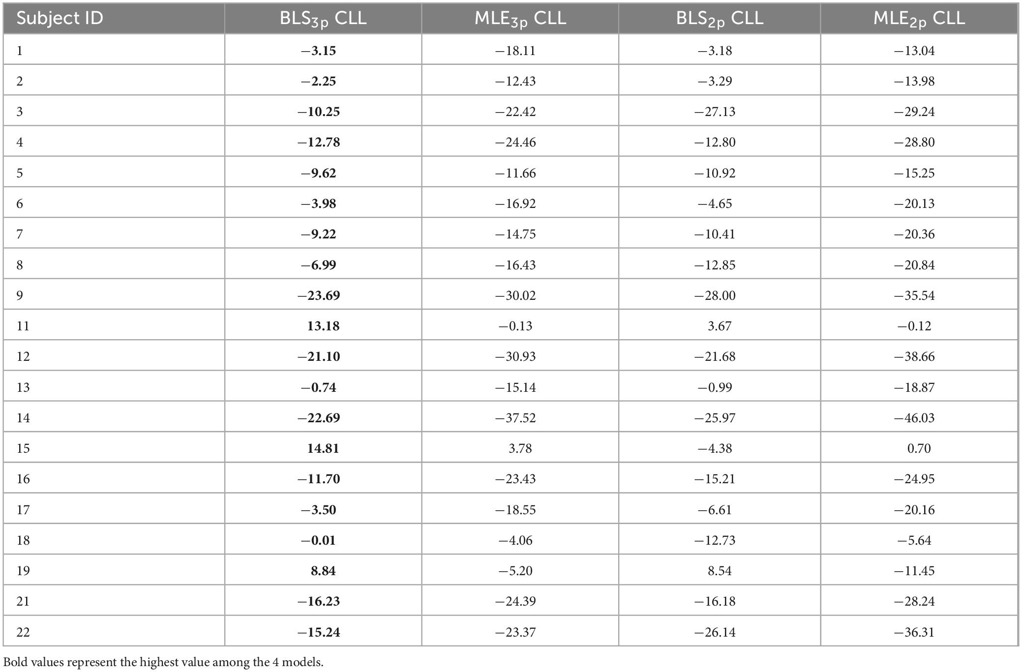
Table 1. Cross-validated log-likelihoods (CLL) computed for models with BLS3p, MLE3p, BLS2p, and MLE2p estimators in time perception domain for all subjects.
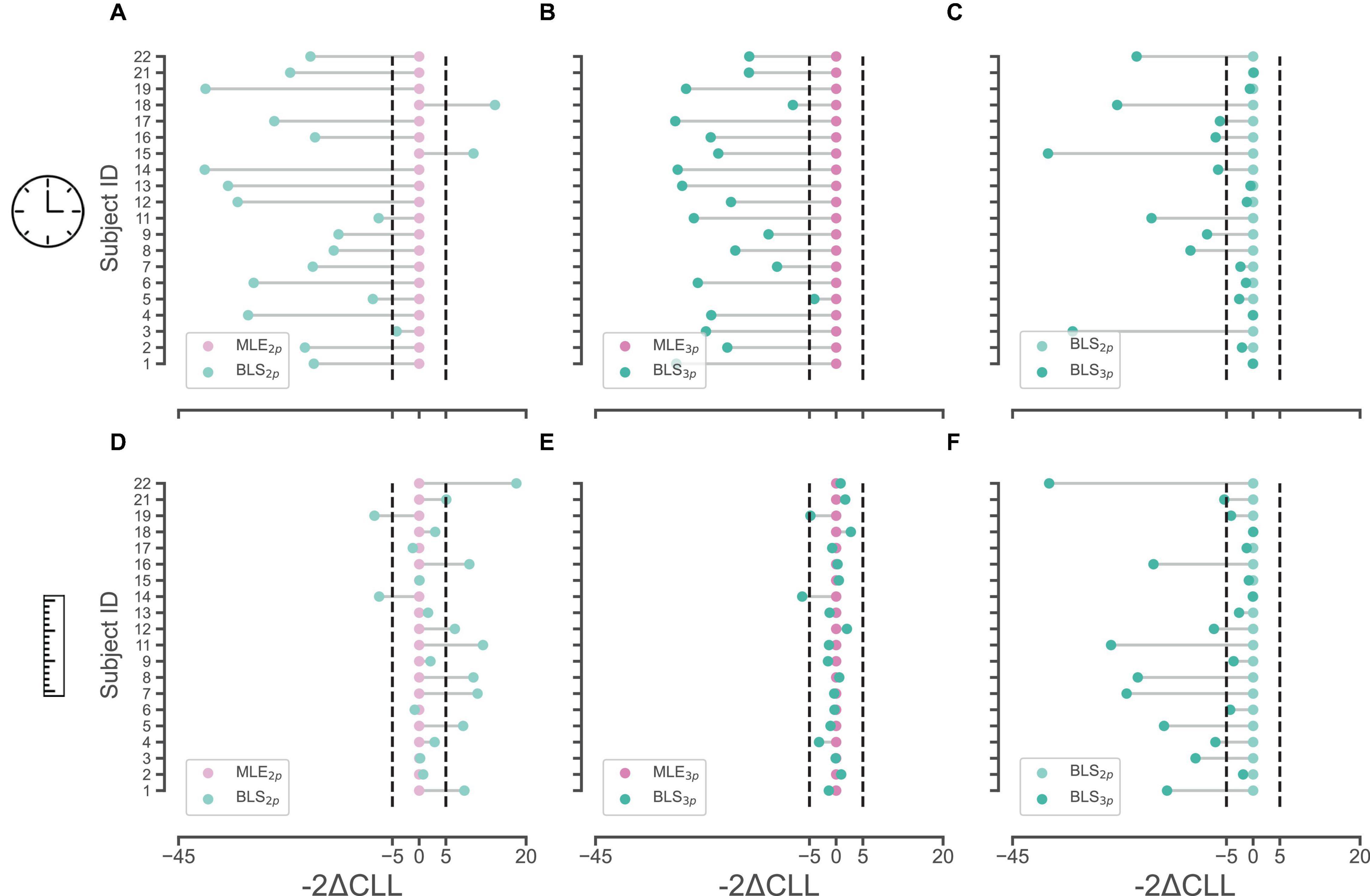
Figure 2. Pair-wise comparisons of observer models with different estimators in time and space. (A,B) Cross-validated log-likelihoods (CLL) were multiplied by 2 and the relative differences of BLS2p (light green) and BLS3p (dark green) models to MLE2p (light pink) and MLE3p (dark pink) models in time domain are plotted, respectively, in (A,B). (C) CLLs were multiplied by 2 and the relative differences of BLS3p (dark green) model to BLS2p (light green) model in time domain is plotted. (D,E) CLLs were multiplied by 2 and the relative differences of BLS2p (light green) and BLS3p (dark green) models to MLE2p (light pink) and MLE3p (dark pink) models in space domain are plotted, respectively, in (D,E). (F) CLLs were multiplied by 2 and the relative differences of BLS3p (dark green) model to BLS2p (light green) model in space domain is plotted. Ordinate represents subject’s ID in each subplot.
In the distance domain, in 55% of subjects, BLS3p was the best fit among our four models as well (11/20, Table 2). In the pairwise comparisons across models, we observed that in only 2/20 subjects BLS2p was a better fit that MLE2p while in 8/20 subjects, MLE2p was a better fit than BLS2p (Figure 2D). Comparing BLS3p and MLE3p did not reveal a conclusive picture (Figure 2E), while BLS3p is a better fit than BLS2p in 11/20 subjects (Figure 2F). These results are plotted as a histogram in Supplementary Figures 1D–F as well. We replicated all of these analyses based on AIC and BIC, and the results were qualitatively similar to CLL data presented here. It seems that both prior-dependent and prior-independent models are capturing the data pattern in space reproduction.
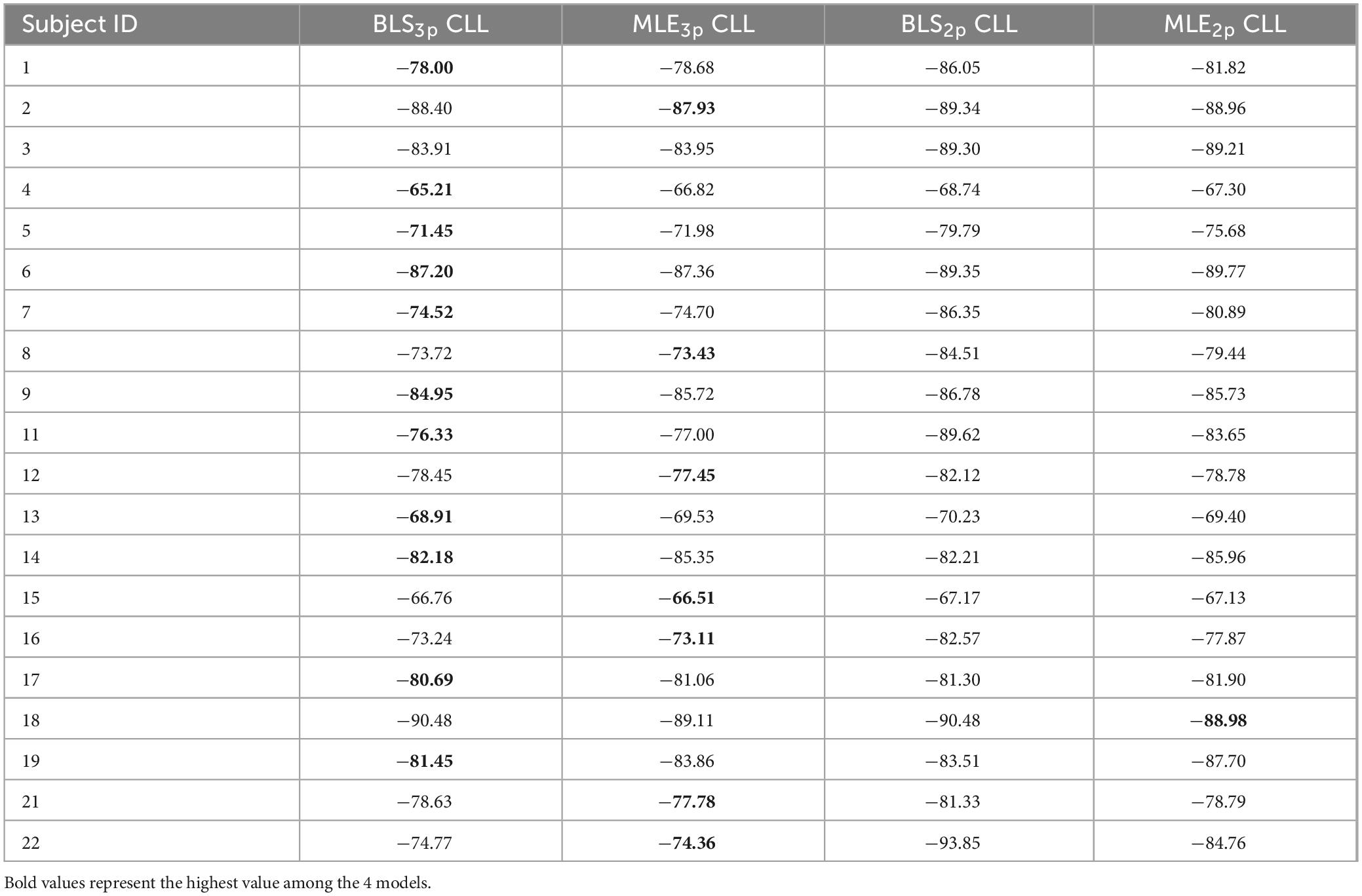
Table 2. Cross-validated log-likelihoods (CLL) computed for models with BLS3p, MLE3p, BLS2p, and MLE2p estimators in space perception domain for all subjects.
We plotted subjects’ reproduced time and distance as a function of the presented duration and distance (Figure 3). In both time and distance, we observed that reproduced time and distance roughly followed the presented time and distance, respectively. In order to observe the goodness-of-fit across our four models (BLS2p, BLS3p, MLE2p, MLE3p), we fitted these models to our data, separately, and plotted simulations from the best fitted models on our data. As it is visually evident, the BLS models outperformed MLE models in the time domain (Figure 3A). In the distance domain (Figure 3B), MLE and BLS models were very similar. So, the results implicate that both prior-dependent models outperformed the prior-independent models in the time perception domain.
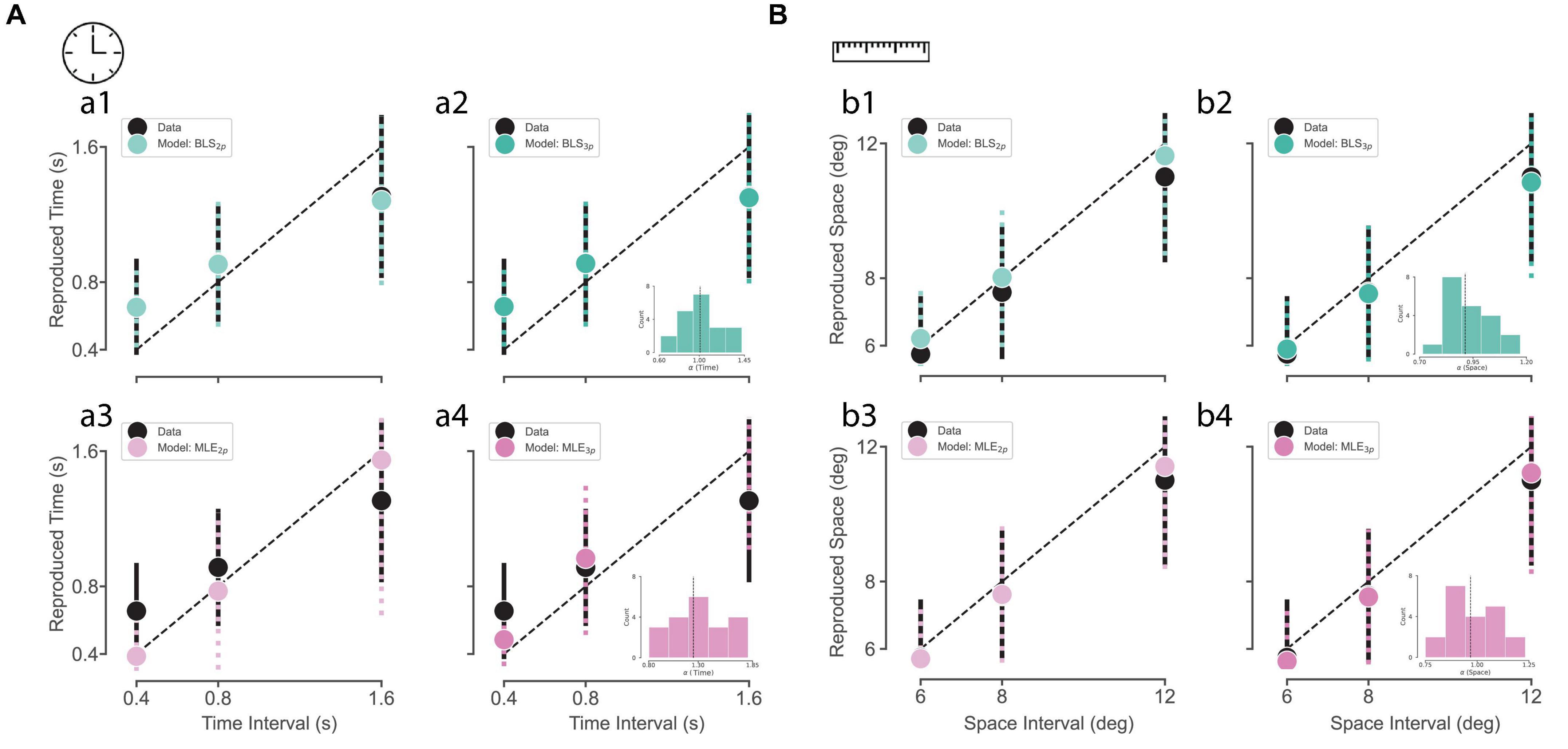
Figure 3. Subjects and observer model behavior in time reproduction (A) and distance reproduction tasks (B). (a1–a4) Black circles and the error bar show the mean ± SD of subjects’ reproduced times across three sample intervals. The colored circles and the dotted error bar indicate the mean ± SD of the Bayesian observer model reproduced times computed from simulations of the best-fitted models with 4 estimators (BLS3p, BLS2p, MLE3p, MLE2p, respectively). (b1–b4) Black circles and the error bar show the mean ± SD of subjects’ reproduced distances across three sample intervals. The colored circles and the dotted error bar indicate the mean ± SD of the Bayesian observer model reproduced distances computed from simulations of the best-fitted models with 4 estimators, BLS2p, BLS3p, MLE2p, and MLE3p, respectively. The inset in (a2, a4, b2, b4) shows the distribution of alpha values for all subjects. The dotted line represents the median of alpha distribution.
3.2 Comparison of model parameters between time and space
Given our results so far, we compared the best fitted free parameters from BLS3p model between time and space. In the case of α we did not find neither correlation (r = −0.11, p = 0.64, Figure 4A), nor difference between time (mean ± SD: 1.01 ± 0.21) and space (0.93 ± 0.11; W = 70, p = 0.2, Wilcoxson Rank Sum). We calculated the measurement (wm) and the reproduction (wr) noise parameters of space and time models (Figure 4B). wm in space domain (0.05 ± 0.03) was lower than wm in time domain (0.30 ± 0.07; W = 210, p < 0.0001). We also found that wr in space domain (0.23 ± 0.02) was smaller than wr in time domain (0.29 ± 0.07; W = 185, p < 0.001). We found that although there was no correlation between wm in space and time domain (r = 0.4, p = 0.08, Figure 4C), there was a positive and significant correlation between wr in time and space domain (r = 0.45, p < 0.05, Figure 4D). These results show that time and space differ in terms of measurement noise while share similar noise profile in reproduction.
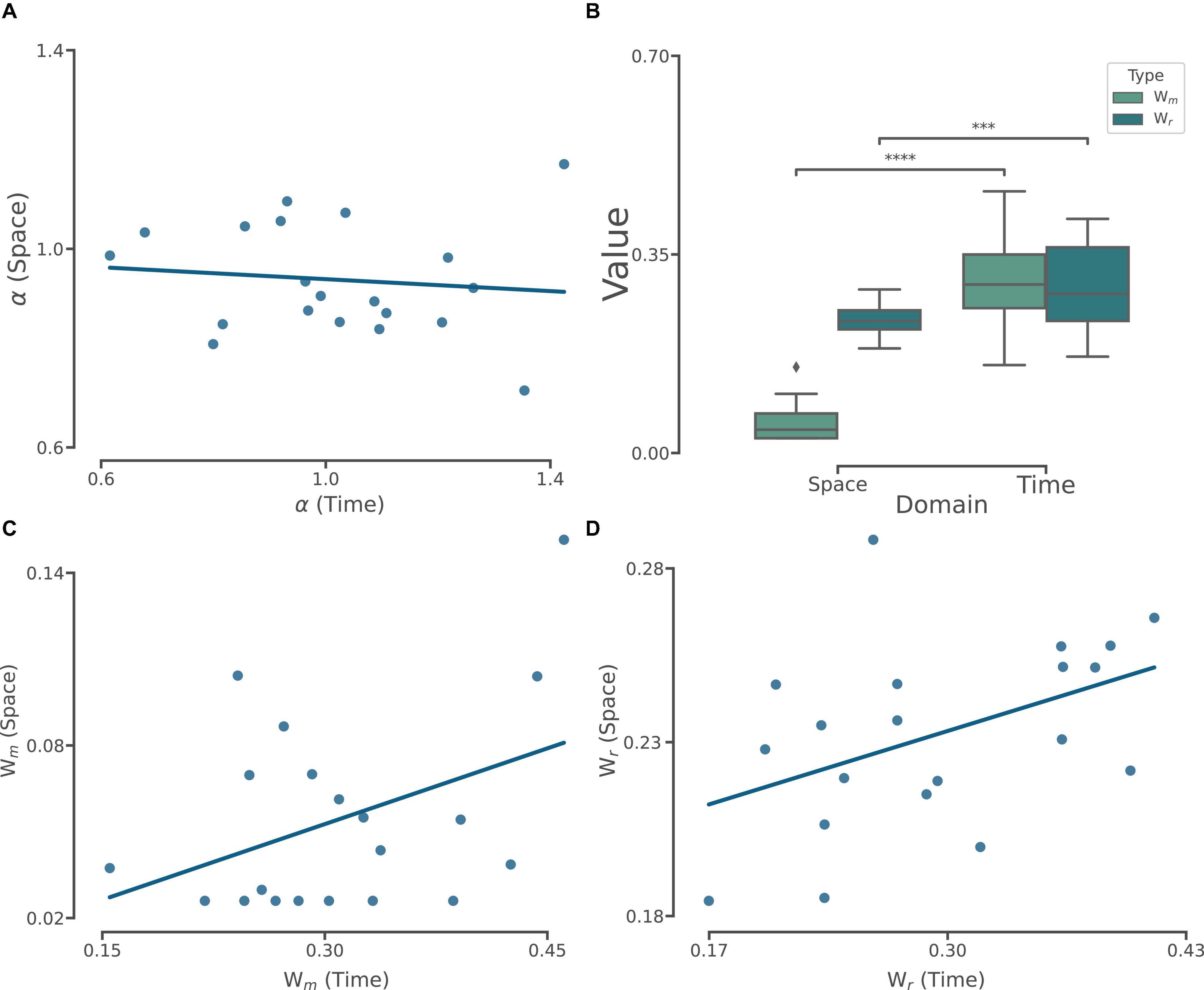
Figure 4. Comparison of and correlation between best fitted model parameters computed in time and space. (A) The correlation (r = –0.11, p = 0.64) between alpha computed from the BLS3p model in time and space. (B) Box plot comparing the distribution of best-fitted model noise parameters between time and space. The line inside the box represents the median, and the whiskers extend to the most extreme data points within 1.5 times the inter-quartile range (IQR). The Wilcoxon signed rank test was conducted to assess the statistical significance of the differences between best-fitted model noise parameters in time and space. p < 0.001***, p < 0.0001****. (C) The correlation (r = 0.40, p = 0.08) between wm computed from the BLS3p model in time and space. (D) The correlation (r = 0.45, p < 0.05) between wr computed from the BLS3p model in time and space.
3.3 Effect of eccentricities/delays on the perception of time/distance intervals
We plotted the reproduced time intervals across different eccentricities (Figure 5A). In order to see whether time perception was dependent on distance, we performed a two-way ANOVA on the reproduced time intervals as a dependent variable (factor 1: eccentricity, factor 2: time interval). We found that both time interval (as expected, F = 1,961.0, df = 2, p < 0.001) and eccentricity (F = 26.1, df = 2, p < 0.001) had a significant effect on the reproduced time interval. The interaction between eccentricity and time interval did not reach a significant level (F = 0.5, df = 4, p = 0.7). This means that as the eccentricity of the stimulus increases, subjects’ perceived time increases as well.
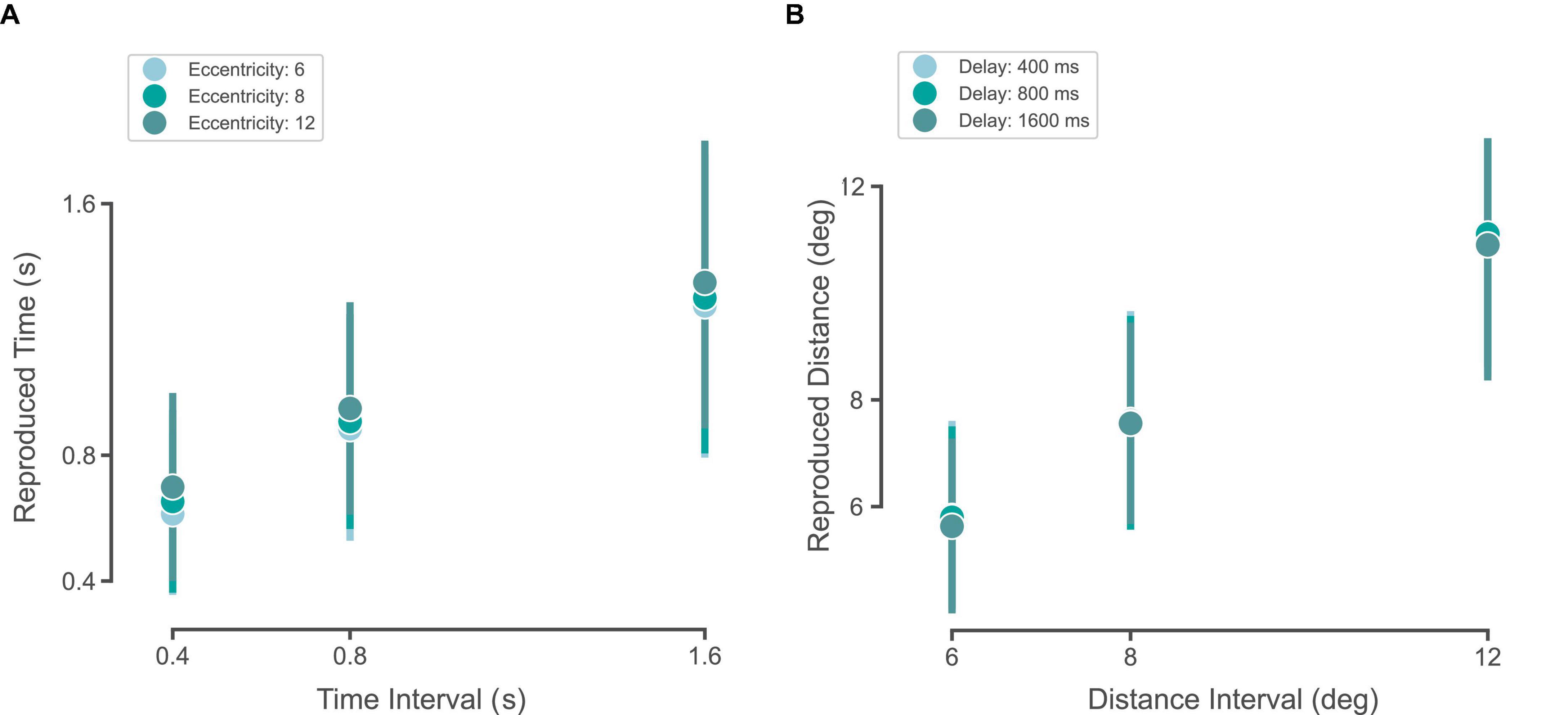
Figure 5. Time-space interference. (A) Circles and the error bar show the mean ± SD of subjects’ reproduced times across three sample intervals for eccentricities of 6 (gray), 8 (green), 12° (cyan). (B) Circles and the error bar show the mean ± SD of subjects’ reproduced distances across three delays of 400 (gray), 800 (green), 1,600 ms (cyan).
For the distance reproduction task, we plotted the reproduced distance intervals across different delays (Figure 5B). In order to see whether space perception was dependent on time, we performed a two-way ANOVA on the reproduced distance intervals as a dependent variable (factor 1: delay, factor 2: distance interval). We found that while distance had a significant effect (as expected, F = 4,073.9, df = 2, p < 0.001), delay did not have any significant effect on the reproduced distance intervals (F = 2.2, df = 2, p = 0.1). The interaction between delay and distance interval did not reach a significant level (F = 0.3, df = 4, p = 0.8). This means that the increase in the delay before response did not affect subjects’ perceived distance.
To further investigate these observations, we took a modeling approach. We fitted BLS3p on the timing data as a function of stimulus eccentricity and used the fitted parameters for simulation across the three eccentricities (6, 8, and 12°). We computed R2 score to assess the goodness-of-fit of a model trained on one eccentricity and tested on other eccentricities. The mean of R2 values is shown in Figure 6A. As can be seen, although each model from any eccentricities can predict data from other eccentricities well (R2s > 0.83), data from each eccentricity predicted the same eccentricity better than others (the rightward diagonal in Figure 6A). Similarly in the space domain, we fitted BLS3p on the space data as a function of delay and used the fitted parameters for simulation across the three delays. We computed R2 score to assess the goodness-of-fit of a model trained on one delay and tested on other delays (R2s > 0.93). The mean of R2 values is shown in Figure 6B. We did not find any systematic difference between models and data as a function of eccentricity. The modeling approach confirmed the ANOVA results.
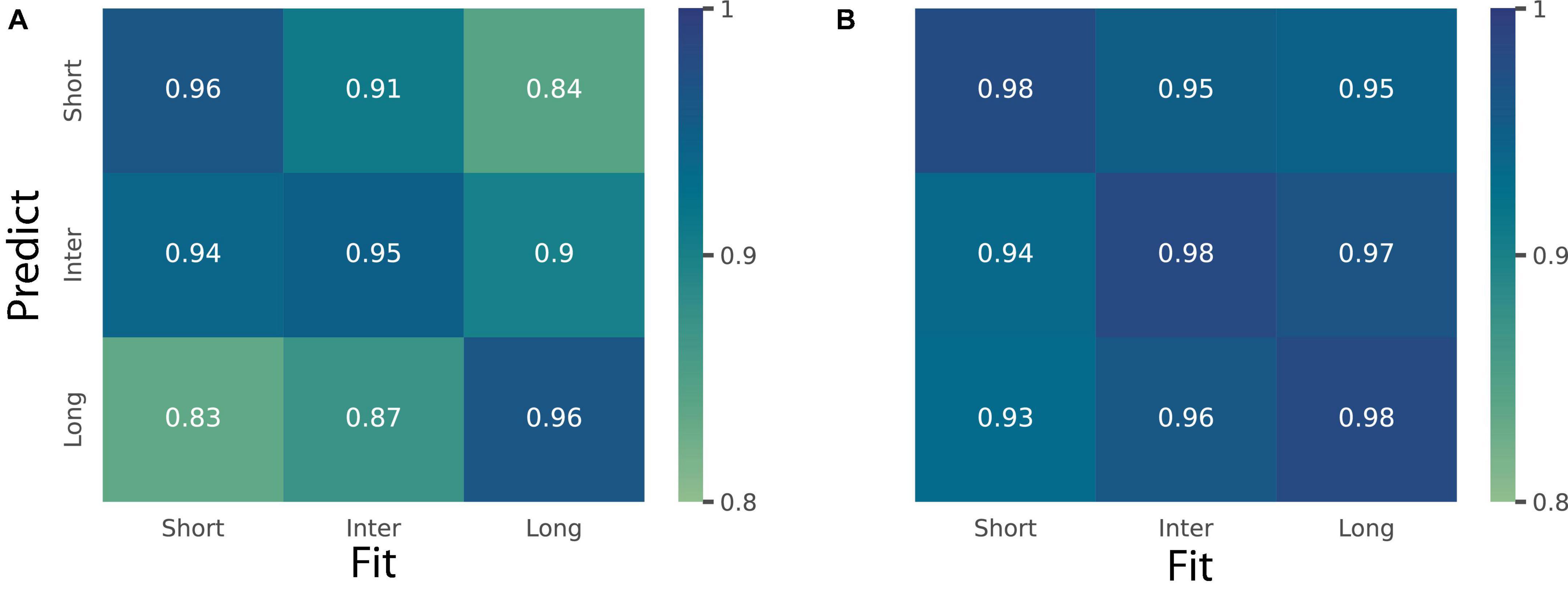
Figure 6. Prediction of a perceptual domain as a function of another one. (A) Heatmap shows R2 values for the simulated Bayesian observer model (BLS3p) for time domain fitted on trials with short (6°), inter (8°), and long (12°) stimulus eccentricity and tested on trials with these eccentricities. (B) Heatmap shows R2 values for the simulated Bayesian observer model (BLS3p) for distance fitted on trials with short (0.4 s), inter (0.8 s), and long (1.6 s) fixation to GO delays and tested on trials with these delays.
4 Discussion
We investigated the similarities and differences in the perception of time and space, as two components of the “A Theory of Magnitude” (ATOM) proposal (Walsh, 2003). Our investigation was motivated by the evidence regarding various encoding schemes that are recruited for time and space across different parts of the brain (Kraus et al., 2013; Marcos et al., 2017; Abramson et al., 2023). To achieve this goal, we designed two magnitude reproduction tasks and made them as much similar in terms of stimuli and procedure as possible. We used the observer model, which (Jazayeri and Shadlen, 2010) had used, with two different estimators [Bayesian least square (BLS) vs. maximum likelihood estimator (MLE)] to our behavioral data. We showed that adding another parameter (α) to the classic Bayesian observer model (Jazayeri and Shadlen, 2010) resulted in better fits regardless of the estimator used. We added α to the ideal observer model in order to capture the heterogeneity of perception of time and space in population (Matthews and Meck, 2014).
We showed that in the time domain, models that take priors into account (i.e., BLS2p and BLS3p) outperformed those that do not (i.e., MLE2p and MLE3p). In the space domain, it remains inconclusive whether MLE3p or BLS3p better captures our data. Since both of these two models in the space domain fitted data well, we chose BLS3p to compare the time and space with the same model. Given that a probabilistic framework explained both time and space, we believe there is a general computation principle in both domains. Although time and space perception abide by shared principles, based on our observation, we believe that this probabilistic computation is applied differently in these two domains: time perception is prior-dependent, while we cannot say the same for space perception.
Our results are corroborated by studies that have shown an effect of global context in time. We provide evidence of the effect of global context on space perception in line with previous works as well (Martin et al., 2017; Sadibolova and Terhune, 2022; Wang et al., 2023). However, we also show that not taking into account the prior would also describe the data equally well. The lack of difference between prior-dependent and prior-independent models in explaining the data in space perception points out to a new challenge in the study of space perception. Space takes different meanings in cognitive experiments (eccentricity in the retinotopic map, surface, distance in navigation, etc.). It may be that priors have an effect on some measures of space and not on the other. Or maybe, the degree of effect varies in different spatial contexts.
Our results are supported by biological evidence as well. A recent meta-analysis has shown that although time and space perception share common regions in the brain, their processing might be separated by an anatomical anterior-posterior gradient (Cona et al., 2021). Dissociable neural indices for time and space have also been found in human electroencephalography (EEG) data (Robinson and Wiener, 2021). Neural recordings from prefrontal cortex (PFC) and temporal lobe in epileptic patients found neurons that encode time-only, space-only or both time and space. In non-human primates, researchers found that neurons in the PFC that encode time and space have a small overlap with each other (Marcos et al., 2017) and the commonality may be at the level of goal coding. These results can be explained by the recent proposal that the brain uses distinct mechanisms to measure temporal and spatial magnitudes and combines them in a unimodal estimate through another mechanism (Gladhill et al., 2022).
In the time domain, we observed in subjects with the lowest and the highest α values, α captured the overall overestimation (Subject No. 3, Supplementary Figure 2) and underestimation (Subject No. 17, Supplementary Figure 3) in time reproduction behavior, respectively. We suggest that α represents the speed of an internal clock (Meck, 1983). Research has shown that people experience the passage of time in different ways and the speed of the internal clock varies in population (Wearden et al., 1999; Allman et al., 2014). Some attempts have been made to use drift diffusion models (DDM) to describe data from timing tasks (Simen et al., 2011). In line with this view, we can reformulate time reproduction as a decision of when to act. The timing of a decision has been studied extensively in the decision-making literature by incorporating an evidence-independent urgency signal to the accumulation of evidence (Cisek et al., 2009; Carland et al., 2016; Ferrucci et al., 2021). An alternative interpretation of α in the perception time is that α could be representative of an urgency signal. The heterogeneity that we found in the performance of our subjects in time reproduction might be linked to their different levels of urgency to act.
In the space domain, we made the same observation regarding α. However, the majority of subjects had α values under 1 (median of 0.9 for the distribution of α) which translates into an overall underestimation tendency in distance reproduction. This observation is in line with previous report of an average undershoot of about 10% of target eccentricity in peripheral saccades (Vitu et al., 2017).
We observed that wm and wr, model parameters representing the level of variability, were lower in space than in time models. We also found that wm was not correlated between time and space which hints at the possibility of different measurement mechanisms in the two domains. One explanation for the observed difference in wm between the two domains could be that there are various sources of variability for time and space, and the measurement and reproduction of space goes under less noisy stages (or processed further). This difference between time and space can be due to how these dimensions are represented in the brain. We believe that given that brain has many retinotopic maps in which spatial relations such as eccentricity, and distance are coded (Felleman and Van Essen, 1991), it has the power to reduce noise at the level of measurement. On the other hand, time has very few chronotopic maps (Protopapa et al., 2019), so the perception of time would be subject to more noise than space. At the motor level, it has long been known that the primate brain has a dedicated system for saccadic eye movement that direct eyes to different locations (Rucci et al., 2007). This system is very precise in transforming static visual scenes into spatiotemporal signals for the brain to structure the spatial maps of the environment (Rucci and Poletti, 2015). We believe that that is the reason why where to look is less noisy than when to look.
We can compute distance based on information from both egocentric cues (i.e., navigation) and distance from fovea (allocentric, i.e., making a saccade) (Feigenbaum and Rolls, 1991; Sabes et al., 2002; Olson, 2003). Distance reproduction tasks so far have mostly focused on egocentric representation as studies have been conducted in virtual reality settings (Maruhn et al., 2019; Zhang et al., 2021). We used a task design in which the perceived and reproduced distances represent the allocentric mapping of spatial information. In recent years, research has found that there are neurons that encode egocentric spatial representations and also represent allocentric spatial relations in primate hippocampal formation (Baraduc et al., 2019; Courellis et al., 2019) driven by saccadic eye movements during visual exploration of environment (Killian et al., 2012). Because of this similarity, we believe our results could generalize to tasks that measure the egocentric encoding of distance.
We observed that as the eccentricity of stimulus increased, the subjects overestimated time intervals, as represented in different (not statistically though) α values obtained from models fitted based on eccentricities we had in our task. We also showed that the fitted parameters to timing data in different eccentricities are not generalizable to other eccentricities, as shown in the deterioration of the goodness-of-fit metric. This finding is in line with the previous observations that as the distance between two visual stimuli, with a constant stimulus onset asynchrony, increases, the perceived duration between these two stimuli also increases. This effect is known as Kappa (Jones and Huang, 1982; Vidaud-Laperrière et al., 2022). On the other hand, the reproduced distances as a function of delay were not different. This observation is unexpected given the literature on the relation of working memory and the anti-saccade task which shows the deterioration of task performance as a function of delay interval (Munoz and Everling, 2004; Meier et al., 2018). We think that the maximum delay duration that we used (1.6 s) is not long enough to manifest the interference effect of time on space.
We do not know that if BLS3p would be a better fit than BLS2p to previously reported data in time domain like the ones from Jazayeri and Shadlen (2010). But although they trained subjects to have a stable performance before their main task, we did not have that training. They also provided feedback regarding the precision of performance to their subjects on each trial, which we did not have that either. So, although we cannot extend our modeling works to theirs, our model is more powerful in dealing with not giving feedback and also not requiring subjects to be heavily trained. Given that our model can accommodate data collection with minimum training, we believe it can be applied more easily in populations for which data collection is an obstacle, like children or people with neurological or psychiatric disorders. Meanwhile, note that we only used three intervals for both time and space (nine conditions) to keep the duration for completing both tasks manageable. We are aware that three intervals might not be enough to generalize our results to larger range of time or space, or other models, that we have not used here, might explain these data more comprehensively. Given the literature on time and space perception, we think this possibility is not likely, but needs further investigation.
Data availability statement
The raw data supporting the conclusions of this article will be made available by the authors, without undue reservation.
Ethics statement
The studies involving humans were approved by the School of Cognitive Sciences, Institute for Research in Fundamental Sciences (IPM). The studies were conducted in accordance with the local legislation and institutional requirements. The participants provided their written informed consent to participate in this study.
Author contributions
SS: Conceptualization, Data curation, Formal analysis, Investigation, Methodology, Software, Supervision, Validation, Visualization, Writing – original draft, Writing – review & editing. MS: Conceptualization, Methodology, Project administration, Supervision, Validation, Writing – review & editing.
Funding
The authors declare that no financial support was received for the research, authorship, and/or publication of this article.
Acknowledgments
We are grateful to Abdol-hossein Vahabie for giving feedback on our data analysis approach, and Mohammad Rabie for comments on a previous version of our manuscript.
Conflict of interest
The authors declare that the research was conducted in the absence of any commercial or financial relationships that could be construed as a potential conflict of interest.
Publisher’s note
All claims expressed in this article are solely those of the authors and do not necessarily represent those of their affiliated organizations, or those of the publisher, the editors and the reviewers. Any product that may be evaluated in this article, or claim that may be made by its manufacturer, is not guaranteed or endorsed by the publisher.
Supplementary material
The Supplementary Material for this article can be found online at: https://www.frontiersin.org/articles/10.3389/fnins.2024.1387641/full#supplementary-material
References
Abramson, S., Kraus, B. J., White, J. A., Hasselmo, M. E., Derdikman, D., and Morris, G. (2023). Flexible coding of time or distance in hippocampal cells. eLife 12:e83930. doi: 10.7554/eLife.83930
Allman, M. J., Teki, S., Griffiths, T. D., and Meck, W. H. (2014). Properties of the internal clock: First- and second-order principles of subjective time. Annu. Rev. Psychol. 65, 743–771. doi: 10.1146/annurev-psych-010213-115117
Baraduc, P., Duhamel, J.-R., and Wirth, S. (2019). Schema cells in the macaque hippocampus. Science 363, 635–639. doi: 10.1126/science.aav5404
Burgess, C., Schuck, N. W., and Burgess, N. (2011). “Chapter 5—temporal neuronal oscillations can produce spatial phase codes,” in Space, Time and Number in the Brain, eds S. Dehaene and E. M. Brannon (Amsterdam: Academic Press), 59–69. doi: 10.1016/B978-0-12-385948-8.00005-0
Buzsáki, G., and Llinás, R. (2017). Space and time in the brain. Science 358, 482–485. doi: 10.1126/science.aan8869
Cai, Z. G., and Connell, L. (2016). On magnitudes in memory: An internal clock account of space–time interaction. Acta Psychol. 168, 1–11. doi: 10.1016/j.actpsy.2016.04.003
Carland, M., Marcos, E., Thura, D., and Cisek, P. (2016). Evidence against perfect integration of sensory information during perceptual decision making. J. Neurophysiol. 115, 915–930. doi: 10.1152/jn.00264.2015
Casasanto, D., and Boroditsky, L. (2008). Time in the mind: Using space to think about time. Cognition 106, 579–593. doi: 10.1016/j.cognition.2007.03.004
Chen, Y., Peng, C., and Avitt, A. (2021). A unifying Bayesian framework accounting for spatiotemporal interferences with a deceleration tendency. Vis. Res. 187, 66–74. doi: 10.1016/j.visres.2021.06.005
Cisek, P., Puskas, G. A., and El-Murr, S. (2009). Decisions in changing conditions: The urgency-gating model. J. Neurosci. 29, 11560–11571. doi: 10.1523/JNEUROSCI.1844-09.2009
Cona, G., Wiener, M., and Scarpazza, C. (2021). From ATOM to GradiATOM: Cortical gradients support time and space processing as revealed by a meta-analysis of neuroimaging studies. NeuroImage 224:117407. doi: 10.1016/j.neuroimage.2020.117407
Courellis, H. S., Nummela, S. U., Metke, M., Diehl, G. W., Bussell, R., Cauwenberghs, G., et al. (2019). Spatial encoding in primate hippocampus during free navigation. PLoS Biol. 17:e3000546. doi: 10.1371/journal.pbio.3000546
Cui, M., Peng, C., Huang, M., and Chen, Y. (2022). Electrophysiological evidence for a common magnitude representation of spatiotemporal information in working memory. Cereb. Cortex 32, 4068–4079. doi: 10.1093/cercor/bhab466
Feigenbaum, J. D., and Rolls, E. T. (1991). Allocentric and egocentric spatial information processing in the hippocampal formation of the behaving primate. Psychobiology 19, 21–40. doi: 10.1007/BF03337953
Felleman, D. J., and Van Essen, D. C. (1991). Distributed hierarchical processing in the primate cerebral cortex. Cereb. Cortex 1, 1–47. doi: 10.1093/cercor/1.1.1-a
Ferrucci, L., Genovesio, A., and Marcos, E. (2021). The importance of urgency in decision making based on dynamic information. PLoS Comput. Biol. 17:e1009455. doi: 10.1371/journal.pcbi.1009455
Gladhill, K. A., Robinson, E. M., Stanfield-Wiswall, C., Bader, F., and Wiener, M. (2022). Anchors for time, distance, and magnitude in virtual movements. bioRxiv [Preprint] doi: 10.1101/2022.09.12.507649
Goldreich, D. (2007). A Bayesian perceptual model replicates the cutaneous rabbit and other tactile spatiotemporal illusions. PLoS One 2:e333. doi: 10.1371/journal.pone.0000333
Howard, M. W., MacDonald, C. J., Tiganj, Z., Shankar, K. H., Du, Q., Hasselmo, M. E., et al. (2014). A unified mathematical framework for coding time, space, and sequences in the hippocampal region. J. Neurosci. 34, 4692–4707. doi: 10.1523/JNEUROSCI.5808-12.2014
Jazayeri, M., and Shadlen, M. N. (2010). Temporal context calibrates interval timing. Nat. Neurosci. 13:8. doi: 10.1038/nn.2590
Jie, Y. U., and Youguo, C. (2023). Spatiotemporal interference effect: An explanation based on Bayesian models. Adv. Psychol. Sci. 31:597. doi: 10.3724/SP.J.1042.2023.00597
Jones, B., and Huang, Y. L. (1982). Space-time dependencies in psychophysical judgment of extent and duration: Algebraic models of the tau and kappa effects. Psychol. Bull. 91, 128–142. doi: 10.1037/0033-2909.91.1.128
Killian, N. J., Jutras, M. J., and Buffalo, E. A. (2012). A map of visual space in the primate entorhinal cortex. Nature 491:7426. doi: 10.1038/nature11587
Kraus, B. J., Robinson, R. J., White, J. A., Eichenbaum, H., and Hasselmo, M. E. (2013). Hippocampal “time cells”: Time versus path integration. Neuron 78, 1090–1101. doi: 10.1016/j.neuron.2013.04.015
Ma, W. J., Kording, K. P., and Goldreich, D. (2023). Bayesian Models of Perception and Action: An Introduction. Cambridge, MA: MIT press.
Marcos, E., and Genovesio, A. (2017). Interference between space and time estimations: From behavior to neurons. Front. Neurosci. 11:631. doi: 10.3389/fnins.2017.00631
Marcos, E., Tsujimoto, S., and Genovesio, A. (2017). Independent coding of absolute duration and distance magnitudes in the prefrontal cortex. J. Neurophysiol. 117, 195–203. doi: 10.1152/jn.00245.2016
Martin, B., Wiener, M., and van Wassenhove, V. (2017). A Bayesian perspective on accumulation in the magnitude system. Sci. Rep. 7:1. doi: 10.1038/s41598-017-00680-0
Maruhn, P., Schneider, S., and Bengler, K. (2019). Measuring egocentric distance perception in virtual reality: Influence of methodologies, locomotion and translation gains. PLoS One 14:e0224651. doi: 10.1371/journal.pone.0224651
Matthews, W. J., and Meck, W. H. (2014). Time perception: The bad news and the good. Wiley Interdiscip. Rev. Cogn. Sci. 5, 429–446. doi: 10.1002/wcs.1298
Meck, W. H. (1983). Selective adjustment of the speed of internal clock and memory processes. J. Exp. Psychol. Anim. Behav. Process. 9, 171–201.
Meier, M. E., Smeekens, B. A., Silvia, P. J., Kwapil, T. R., and Kane, M. J. (2018). Working memory capacity and the antisaccade task: A microanaltyic-macroanalytic investigation of individual differences in goal activation and maintenance. J. Exp. Psychol. Learn. Mem. Cogn. 44, 68–84. doi: 10.1037/xlm0000431
Morrone, M. C., Ross, J., and Burr, D. (2005). Saccadic eye movements cause compression of time as well as space. Nat. Neurosci. 8, 950–954. doi: 10.1038/nn1488
Munoz, D. P., and Everling, S. (2004). Look away: The anti-saccade task and the voluntary control of eye movement. Nat. Rev. Neurosci. 5:3. doi: 10.1038/nrn1345
Olson, C. R. (2003). Brain representation of object-centered space in monkeys and humans. Annu. Rev. Neurosci. 26, 331–354. doi: 10.1146/annurev.neuro.26.041002.131405
Petzschner, F. H., and Glasauer, S. (2011). Iterative Bayesian estimation as an explanation for range and regression effects: A study on human path integration. J. Neurosci. 31, 17220–17229. doi: 10.1523/JNEUROSCI.2028-11.2011
Protopapa, F., Hayashi, M. J., Kulashekhar, S., van der Zwaag, W., Battistella, G., Murray, M. M., et al. (2019). Chronotopic maps in human supplementary motor area. PLoS Biol. 17:e3000026. doi: 10.1371/journal.pbio.3000026
Robbe, D. (2023). Lost in time: Relocating the perception of duration outside the brain. Neurosci. Biobehav. Rev. 153:105312. doi: 10.1016/j.neubiorev.2023.105312
Robinson, E. M., and Wiener, M. (2021). Dissociable neural indices for time and space estimates during virtual distance reproduction. NeuroImage 226:117607. doi: 10.1016/j.neuroimage.2020.117607
Rucci, M., Iovin, R., Poletti, M., and Santini, F. (2007). Miniature eye movements enhance fine spatial detail. Nature 447, 851–854. doi: 10.1038/nature05866
Rucci, M., and Poletti, M. (2015). Control and functions of fixational eye movements. Annu. Rev. Vis. Sci. 1, 499–518. doi: 10.1146/annurev-vision-082114-035742
Sabes, P. N., Breznen, B., and Andersen, R. A. (2002). Parietal representation of object-based saccades. J. Neurophysiol. 88, 1815–1829. doi: 10.1152/jn.2002.88.4.1815
Sadibolova, R., and Terhune, D. B. (2022). The temporal context in Bayesian models of interval timing: Recent advances and future directions. Behav. Neurosci. 136, 364–373. doi: 10.1037/bne0000513
Safaie, M., Jurado-Parras, M.-T., Sarno, S., Louis, J., Karoutchi, C., Petit, L. F., et al. (2020). Turning the body into a clock: Accurate timing is facilitated by simple stereotyped interactions with the environment. Proc. Nat. Acad. Sci. U. S. A. 117, 13084–13093. doi: 10.1073/pnas.1921226117
Schonhaut, D. R., Aghajan, Z. M., Kahana, M. J., and Fried, I. (2023). A neural code for time and space in the human brain. Cell Rep. 42:113238. doi: 10.1016/j.celrep.2023.113238
Schroeger, A., Raab, M., and Cañal-Bruland, R. (2022). Tau and kappa in interception – how perceptual spatiotemporal interrelations affect movements. Attent. Percept. Psychophys. 84, 1925–1943. doi: 10.3758/s13414-022-02516-0
Schwertman, N. C., Owens, M. A., and Adnan, R. (2004). A simple more general boxplot method for identifying outliers. Comput. Stat. Data Anal. 47, 165–174. doi: 10.1016/j.csda.2003.10.012
Simen, P., Balci, F., deSouza, L., Cohen, J. D., and Holmes, P. (2011). A model of interval timing by neural integration. J. Neurosci. 31, 9238–9253. doi: 10.1523/JNEUROSCI.3121-10.2011
Thurley, K., and Schild, U. (2018). Time and distance estimation in children using an egocentric navigation task. Sci. Rep. 8:18001. doi: 10.1038/s41598-018-36234-1
Üstün, S., Sırmatel, B., and Çiçek, M. (2022). Can a common magnitude system theory explain the brain representation of space, time, and number? Noro Psikiyatri Arsivi 59(Suppl. 1), S24–S28. doi: 10.29399/npa.28159
Vidaud-Laperrière, K., Brunel, L., Syssau-Vaccarella, A., and Charras, P. (2022). Exploring spatiotemporal interactions: On the superiority of time over space. Attent. Percept. Psychophys. 84, 2582–2595. doi: 10.3758/s13414-022-02546-8
Vitu, F., Casteau, S., Adeli, H., Zelinsky, G. J., and Castet, E. (2017). The magnification factor accounts for the greater hypometria and imprecision of larger saccades: Evidence from a parametric human-behavioral study. J. Vis. 17:2. doi: 10.1167/17.4.2
Walsh, V. (2003). A theory of magnitude: Common cortical metrics of time, space and quantity. Trends Cogn. Sci. 7, 483–488. doi: 10.1016/j.tics.2003.09.002
Wang, T., Luo, Y., Ivry, R. B., Tsay, J. S., Pöppel, E., and Bao, Y. (2023). A unitary mechanism underlies adaptation to both local and global environmental statistics in time perception. PLoS Comput. Biol. 19:e1011116. doi: 10.1371/journal.pcbi.1011116
Wearden, J. H., Philpott, K., and Win, T. (1999). Speeding up and (…relatively…) slowing down an internal clock in humans. Behav. Process. 46, 63–73. doi: 10.1016/S0376-6357(99)00004-2
Whitaker, M. M., Hansen, R. C., Creem-Regehr, S. H., and Stefanucci, J. K. (2022). The relationship between space and time perception: A registered replication of Casasanto and Boroditsky (2008). Attent. Percept. Psychophys. 84, 347–351. doi: 10.3758/s13414-021-02420-z
Keywords: time, space, perception, Bayesian, spatiotemporal
Citation: Sima S and Sanayei M (2024) Same principle, but different computations in representing time and space. Front. Neurosci. 18:1387641. doi: 10.3389/fnins.2024.1387641
Received: 18 February 2024; Accepted: 11 April 2024;
Published: 07 May 2024.
Edited by:
Ernest Greene, University of Southern California, United StatesReviewed by:
Pierfrancesco Ambrosi, Stella Maris Foundation (IRCCS), ItalyEncarni Marcos, Instituto de Neurociencias Alicante, Spain
Copyright © 2024 Sima and Sanayei. This is an open-access article distributed under the terms of the Creative Commons Attribution License (CC BY). The use, distribution or reproduction in other forums is permitted, provided the original author(s) and the copyright owner(s) are credited and that the original publication in this journal is cited, in accordance with accepted academic practice. No use, distribution or reproduction is permitted which does not comply with these terms.
*Correspondence: Mehdi Sanayei, mehdi.sanayei@gmail.com