Flow control in a confined supersonic cavity flow using subcavity

1 Introduction

Confined cavities exhibit a wide array of applications in the aerospace industry (Sahoo et al. (2005); Emmert et al. (2009); Johnson and Papamoschou (2010); Chakravarthy et al. (2018); Devaraj et al. (2020); Saravanan et al. (2020); Sekar et al. (2020)). They accommodate fuel tanks, payloads, and resonator-type nozzles and are also used in thermal management for spacecraft and aircraft and in propulsion systems, for instance, scramjet combustors Krishnamurty (1955) Rossiter (1964) Heller et al. (1971). The speed of the freestream air at the cavity opening and the length-to-depth ratio of the cavity actively influence cavity flows. Previous categorizations of cavities distinguished between deep and shallow cavities based on the length-to-depth ratio. Based on the static pressure distribution on the cavity floor, cavities are classified as open, closed, or transitional. Stallings and Wilcox (1987) studied cavities on supersonic flow boundaries and concluded that deep cavities exhibit open flow, while shallow cavities exhibit closed flow. Deep cavities, characterized by a length-to-depth ratio less than or equal to 10, result in the shear layer from the leading edge impinging on the trailing edge without entering the cavity and are therefore referred to as open cavities. Shallow cavities, with a length-to-depth ratio greater than 13, display closed flow, where the shear layer from the leading edge impinges on the cavity floor and reattaches before moving downstream to the trailing edge. Cavities with a length-to-depth ratio between 10 and 13 exhibits a transitional flow type. Tracy (1992) and Plentovich et al. (1993) demonstrated that the classification of cavities into open and closed flow types also depends on the width-to-depth ratio. Additionally, the Mach number significantly influences this classification, particularly in supersonic and transonic flows. Lawson and Barakos (2011) stated that the closed cavities do not show any form of acoustic tones. The open cavities, however, possess a distinguished acoustic signature, which consists of the following features:,

1. Low energy broadband noise contributed by the free stream, the shear layer, and turbulent fluctuations.

2. The discrete tones commonly known as the Rossiter modes that vary in magnitude and are usually caused by the vortex-vortex, vortex-wall, vortex-shear layer, shock-shear layer, shear-wall, or any likewise interactions.

Woolley and Karamcheti (1974) Rockwell and Naudascher (1978) have extensively studied the flow in an open cavity and reported that the flow past a supersonic cavity is highly unsteady due to the self-sustaining oscillations existing inside it. The shear layer separates from the leading edge of the cavity, travels downstream, forming large coherent structures, and impinges on the trailing edge. Periodic compression and expansion waves form at the trailing edge, which alternately scavenges the mass in and out of the cavity. The inflow of the mass inside the cavity results in acoustic waves that travel upstream from the base of the cavity to the leading edge and excite the shear layer. This strong coupling between hydrodynamics and acoustics results in a feedback mechanism (Heller and Delfs, 1996). The self-sustaining cavity oscillations are influenced by shear-layer instability, disturbance feedback, resonant wave conditions, and structural elasticity, either individually or in combination.

The oscillations inside the cavity result in undesirable acoustic loading, which can cause severe structural failure Rockwell and Naudascher (1978). Therefore, reducing these oscillations while designing the cavity structures is crucial. Rowley and Williams (2006) provided several noise control techniques and classified them as active and passive control. Active flow control involves the use of external energy sources or actuators to actively manipulate the flow field in real time. They involve active adjustment of control parameters to achieve the desired flow modification, such as modulated pulse jets Abdolahipour et al. (2022b), Abdolahipour et al. (2022a), Abdolahipour et al. (2021), Abdolahipour (2023), plasma actuators Taleghani et al. (2018), and the generation of surface waves Noori et al. (2021) Rahni et al. (2022) and magnetic field Azadi et al. (2023). Passive flow control, on the contrary, relies on the inherent properties of flow-obstructing devices or passive structures to modify the flow behavior without requiring external energy input. Zhuang et al. (2006) used a steady and pulsed injection of mass inside the cavity to reduce the amplitude by 20 dB concerning the cavity tones They also reported a 9 dB reduction in the overall noise intensity. The deposition method of laser energy in the cavity flow adopted by Yilmaz and Aradag (2013) suppresses the noise level up to 7 dB. The studies of Vikramaditya and Kurian (2009) illustrate the effects of angle deflection of the ramp on cavity noise. Their passive control technique of decreasing the angle of the ramp from 90° to 60° reduces the pressure oscillations in the cavity significantly. Researchers have also established that the inflow and outflow of mass inside the cavity are controlled by the compression waves formed at the trailing edge. These compression waves, therefore, play a pivotal role in generating acoustic waves inside the cavity. Malhotra and Vaidyanathan (2016) reported the reduction of sound intensity by incorporating an offset in the aft wall. Lee et al. (2008) inferred that the sub-cavity present at the trailing edge suppresses noises more than adding bumps or blowing techniques. The studies of Alam et al. (2007) on an open supersonic cavity stated that sub-cavities effectively attenuate the cavity’s pressure oscillations. However, the intensity of the suppression of the oscillations depends on the length of the sub-cavity. Lad et al. (2018) experiments showed that the change in the sub-cavity length results in the switching of the oscillation modes from fluid dynamic to fluid resonant mode. These studies establish sub-cavity as a simple and effective passive control for cavity oscillations. Jain and Vaidyanathan (2021) conducted numerical studies on the baseline cavity, featuring a length-to-depth ratio of 2, and investigated two different Mach numbers, namely, 1.71 and 3.25. Since the cavity was not confined between walls, compression waves did not impinge on the shear layer. They explored various lengths of sub-cavities positioned at both the front wall and aft wall, revealing distinct fluid-resonant modes and oscillations. To observe flow features, vortex shedding, and mixing characteristics inside the cavity, they have employed flow visualization techniques such as density gradient-based numerical schlieren, vorticity contours, and streamlines. Their findings suggest that front wall sub-cavities serve as passive control devices, effectively suppressing self-sustained oscillations in cavity configurations. Chavan et al. (2022) conducted experiments on a cavity with a length-to-depth ratio of two and a freestream Mach number of 1.71, along with front wall and aft wall sub-cavities of length ratio 0.2. Their results indicate that the front wall sub-cavity contributes to suppressing cavity oscillations. In another study of Jain et al. (2023), experiments were performed on a cavity with a length-to-depth ratio of two and an inlet Mach number of 1.71. Sub-cavities were added at the floor of the cavity, along with sub-cavities of a length ratio of 0.2 at the front wall and the aft wall. The authors concluded that the floor cavities with the aft wall sub-cavities act as passive resonators, while those with the front wall sub-cavities effectively suppress cavity oscillations. Their experiments were conducted in an unconfined cavity.

In confined cavities, the incoming supersonic flow contains multiple incident and reflected shock waves, comprising the shock train. It forms inside the passage due to the reflection between the wall of the confinement and the shear layer, resulting in an intricate shock-shear layer interaction (Karthick (2021)). The incident shock wave can impinge on the shear layer (based on the operating conditions of the intake) while it is traveling downstream toward the trailing edge. These typical shock shear layer interactions can drastically alter the flow field inside the cavity and above it. Most numerical studies related to cavities mentioned above did not account for this interaction of the cavity shear layer with shock waves, which is otherwise inevitable, especially in scramjet combustors with realistic flow conditions. Hence, it is relevant to consider the shock impingement on the shear layer in the studies of the confined cavity.

The novelty of this article lies in analyzing the confined cavity flow oscillation process in the presence of an impinging shock wave over the shear layer and subsequent behavior with different sub-cavity configurations and their locations concerning the main cavity. The study’s primary objective is to examine and understand the role of sub-cavities placed at the front wall and the aft wall of a supersonic open cavity in controlling the flow oscillations inside a cavity. Numerical simulations aid in exploring the dynamics of supersonic flow within the cavity with a length-to-depth ratio (L/D) of 3. The sub-cavities, with a length-to-cavity-length (l/L) ratio of 0.2, 0.25, and 0.3, serve as a focal point for investigating changes in the flow physics. The investigation is conducted using the Unsteady Reynolds Averaged Navier Stokes equations (URANS) within the OpenFOAM framework. A preliminary investigation of sub-cavities’ effects on the shock-shear layer interaction is also conducted. These interactions are predominant due to the supersonic flow inside the confinement. The ratio of static pressures behind and ahead of the shock (p₂/p₁) is maintained at 1.2. The incoming flow into the cavity operates at a Mach number of 1.71. The study utilizes spectral analysis and numerical flow-field visualization to delve into a deeper investigation of the flow field of the configurations considered.

The remainder of the article is organized as follows: Section 2 discusses the geometrical configuration, numerical methods, boundary conditions, grid independence study, and the validation of the code against the experiments. Section 3 presents the frequency contents of the unsteady signal concerning the different cavity configurations. They are obtained by the Power Spectral Density (PSD) analysis and are further corroborated with the unsteady events inside the cavity visualized using the synthetic Schlieren images. Section 4 summarises the key outcomes of this numerical investigation.

2 Mathematical methodology and flow condition

2.1 Geometrical configuration

The baseline configuration in the present study corresponds to the cavity configuration with a length-to-depth (L/D) ratio of 3. The computational domain extends in the upstream direction by x/D = 5. A ramp at the top wall with the deflection angle (θ) of 3.6° deflects the incoming supersonic flow and produces the leading shock wave angle (β), 39.3°. This shock impinges on the detaching shear layer, and multiple reflections between the constant pressure shear layer and the top wall generate the shock train inside the confinement. The pressure ratio across the oblique impinging shock is maintained at 1.2. The height at the inlet of the duct (H_i) is 1.958 times the depth (D) of the cavity, whereas the outlet height (H_o)is 1.954 times the depth. There are six additional cavity configurations with an additional sub-cavity with a cavity-to-sub-cavity ratio (l/L) of 0.2, 0.25, and 0.3 placed in the middle of the front wall and aft wall of the cavity, while the other parameters are at par with the baseline configuration. Monitoring stations or probes are placed in the midpoint of the front (P1), aft (P2), and bottom (P3) walls of the cavity in all the configurations for recording the unsteady statistics and analyzing them to evaluate the flow field. Figure 1 shows the aforementioned geometrical details.

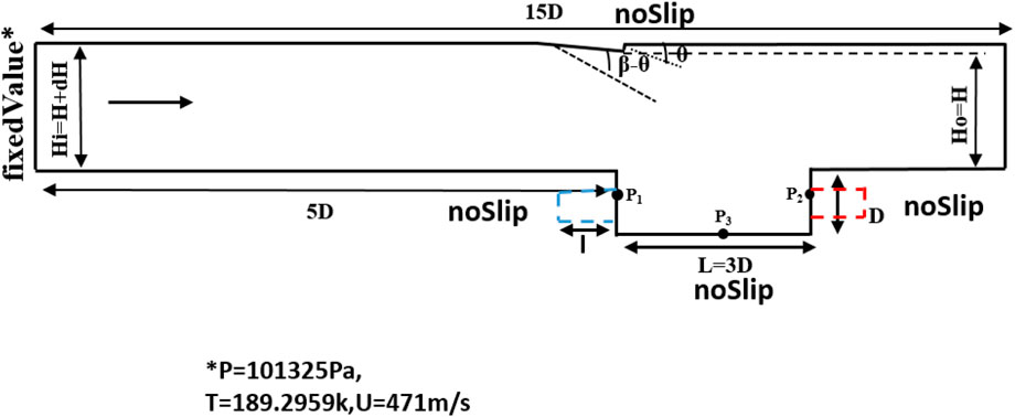
Figure 1. Schematics of Geometry of baseline cavity and the baseline cavity with sub-cavity at the front wall (shown by blue dotted line) and at the aft wall (shown by red dotted line).

2.2 Numerical methodology and boundary conditions

The flow field is simulated using the Unsteady Reynolds Averaged Navier-Stokes equation (URANS) (Versteeg and Malalasekera (2007) Eqs (1)–(3).) which facilitates the resolution of the cavity shear layer’s oscillations and the pressure waves inherent to the cavity flow. These equations produce the average behavior of the fluid flow by separating the temporal mean and fluctuating components of the instantaneous data. They are listed here for convenience.

Here, ρ is the density of the fluid, u_i represents the velocity components, p denotes pressure, and E portrays the total energy of the flow comprising the internal, kinetic, and turbulent kinetic energy.

The eddy viscosity (μ_t) is calculated using the k − ω SST (Shear Stress Transport) turbulence model Menter et al. (2003). This turbulence model combines the strengths of k-ω and k-ϵ models, enhancing accuracy in the boundary layer, separation, and adverse pressure gradient regions. The transport equations of the turbulent kinetic energy and the dissipation rate Eqs 4, 5 are solved along with the Navier-Stokes equation to incorporate the turbulence effects. In these equations, k denotes the turbulent kinetic energy, ω represents the specific dissipation rate, β*, κ, σ_ω, γ, σ_k, σ_m are model constants, and μ and μ_t are the molecular viscosity and the turbulent viscosity, respectively. $\overline{u_i^{\prime }{u}_j^{\prime }}$ denotes the Reynolds stress tensor. P_k represents the production of turbulent kinetic energy, and ɛ denotes the dissipation rate of turbulent kinetic energy.

Further, the specific heat of the air is calculated through the polynomial expression from the Joint Army-Navy-Air Force (JANAF) model Stull (1965) and the viscosity is calculated using Sutherland’s law. The laminar and turbulent thermal conductivity of the medium is derived using the corresponding Prandtl numbers (Pr and Pr_t). The typical values of Pr = 0.72 and Pr_t = 0.8 for air are used in this numerical investigation. The working medium is assumed to obey the ideal gas laws.

The computations of the aforementioned governing equation in the flow field are performed using the density-based Finite Volume Method (FVM) solver ‘rhoEnergyFoam’, in the OpenFOAM framework (Modesti and Pirozzoli, 2017). The convective fluxes in the governing equation are discretized using the AUSM⁺ − up. This formulation ensures the preservation of the total kinetic energy of the flow. The reader is also encouraged to refer to the article by Modesti et al. (Modesti and Pirozzoli, 2017) for this scheme’s description and detailed implementation. Further, the diffusion fluxes are treated using the central scheme, which is second-order accurate in space. The numerical solution advances in time using the low storage, third-order accurate, 4-stage Runge-Kutta time integration method. The inlet of the domain is prescribed with a static pressure and temperature of 101,325 Pa and 189 K at the inlet and a velocity of 471 m/s. The walls are imposed with no-slip conditions and treated as insulated walls. All the variables are extrapolated at the outlet of the domain, assuming the flow to be supersonic. The flow field is initialized with the free stream conditions.

2.3 Validation

The flow conditions tested by Gruber et al. (2001) are used for validating the solver, the fluctuation scales of the turbulence generated explicitly at the inlet, and the steady state flow. Gruber et al. performed their experiments on a deep cavity with a length-to-depth ratio of three under freestream conditions of a Mach number of three and stagnation pressure and temperature of 690 kPa and 300 K, respectively.

2.3.1 Grid independence and solver validation

The computational grids are generated using commercial software, ICEM CFD Ansys (2011). The y⁺ is maintained at less than one to resolve the boundary layer. The grid stretches in both streamwise and transverse directions at a cell-size progression ratio of 1.12, ensuring the cell’s maximum aspect ratio does not exceed 100. Grids with increasing resolutions are tested to obtain an optimal grid size that is accurate and, at the same time, consumes minimal computational resources. A coarse grid of size 1.89∗10⁵, a medium grid of size 5.89∗10⁵, and a fine grid of size 16∗10⁵ are utilized in the present investigation to serve this purpose. Figure 2A depicts the time-averaged pressure, $<p>$, normalized with the freestream pressure, p_∞, measured along the cavity length in the streamwise direction. We observe that the medium and fine grids provide almost the same results. Hence, the medium grid, which is economical for the present study, is used for further analysis of the confined cavities.

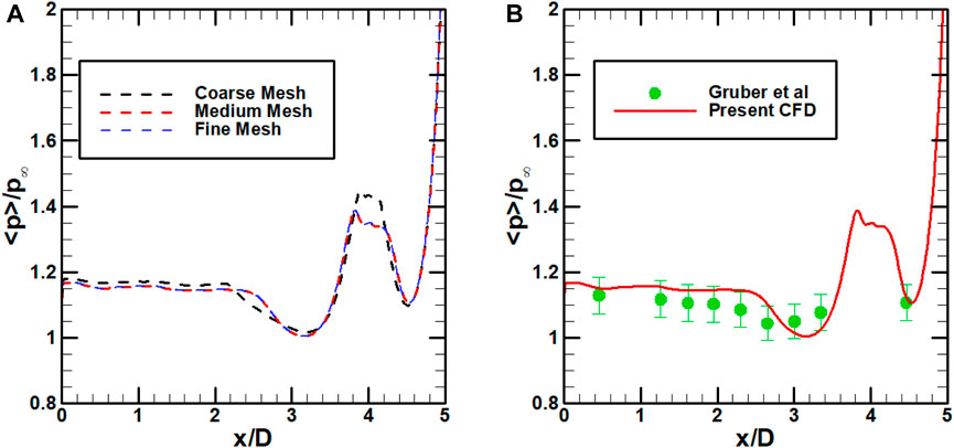
Figure 2. (A) Grid Independence and (B) Validation of the present work against the experiments of Gruber et al. (2001).

The result from the medium grid is validated by comparing the time-averaged pressure distribution obtained against Gruber’s experimental data. Figure 2B shows that the medium grid of the present numerical study is in good agreement with experimental results except near x/D = 4. It is attributed to the exclusion of three-dimensional effects in the present computations. Additionally, there are certain discrepancies in the experimental setup and sensors, as Karthick (2021) mentioned. Nevertheless, the numerical results are within the acceptable tolerance limits concerning the experimental results at all the other locations.

2.3.2 Impact of turbulent intensity

The present study employs the k–ω SST (Shear Stress Transport) turbulence model for the turbulence modeling. The ‘turbulentInlet’ boundary condition in OpenFOAM generates a fluctuating velocity field about the mean velocity field which gives an accurate representation of a turbulent flow at the inlet. In the initial conditions, we define the mean velocity and turbulent intensity. We have varied the turbulent intensity to obtain the most appropriate fluctuating field. For each of these cases, we have also obtained the value of the initial turbulent kinetic energy (as we have considered isotropic turbulence, the turbulent kinetic energy will be equal to 1.5 times the mean square fluctuating velocity field). In this investigation, the turbulent intensity is systematically varied from 3% to 7%. Figure 3 illustrates the outcomes of these variations. The simulations, conducted using a medium-mesh for all cases, reveal that results with a 5% intensity closely align with the experimental data of Gruber. Therefore, an intensity of 5% is used for all the subsequent simulations.

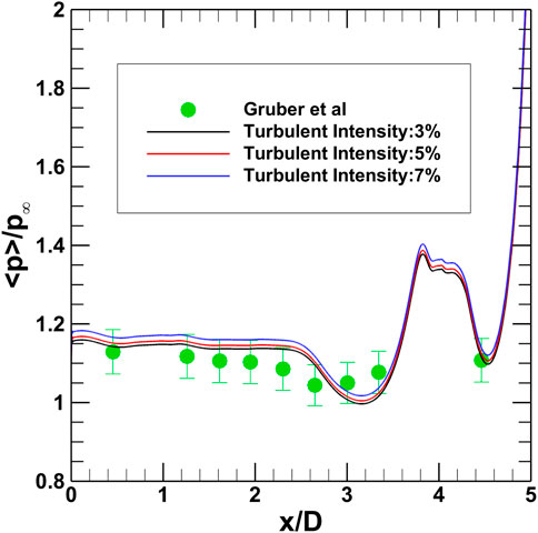
Figure 3. Validation of the turbulent intensity against the experiments of Gruber et al. (2001).

2.3.3 Time step independence and statistically steady state analysis

The solver uses an explicit method for iterating the solution, initially adjusting the physical time step (δt) with the minimum of the convective and thermal diffusion, reflected in the local Courant number or the Courant-Friedrichs-Lewy (CFL) condition. After a considerable number of iterations, the physical time step (δt) gets fixed to a relevant constant value, which is mostly in the order of 1e-09. Data for spectral analysis is then collected at these fixed time intervals. We have used three ‘δt’ of the same order. When the δt is 2e-09 and 3e-09, the results have given a good match with the experiments of Gruber (Figure 4). Hence, we use the δt as 2e-09 for the other simulations.

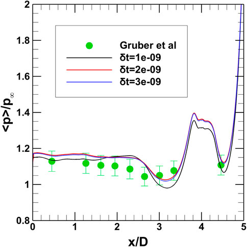
Figure 4. Validation of time step independence against the experiments of Gruber et al. (2001).

The time-averaged pressure obtained from the present numerical simulations, normalized with the freestream pressure along the cavity wall is validated against Gruber’s experimental data (2.3.1). We obtain the mean of the flow variables only after the flow stabilizes. In this simulation, the flow stabilizes after 2.8 ms. We have continued running the numerical simulations until 6 ms. Figure 5 shows that beyond 3 ms, the variation of time-averaged pressure with time is insignificant concerning the medium grid size. This shows that the steady state has been reached. Hence, for subsequent analyses, the relevant data used for further analysis is obtained after 3 ms.

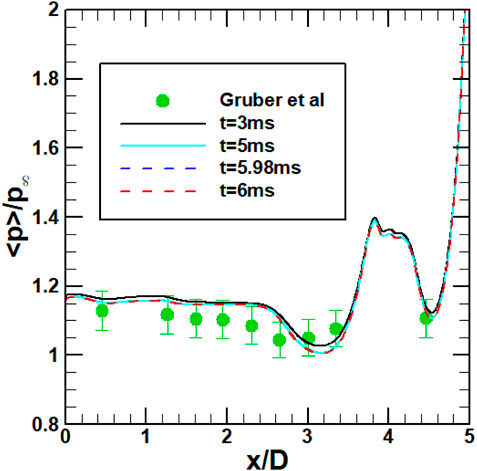
Figure 5. Steady-state validation against the experiments of Gruber et al. (2001).

3 Results and discussion

We have performed flow-field visualization and spectral analysis for each of the configurations to determine the effects of the sub-cavity in the flow field of a confined cavity. Numerical Schlieren images represented by Density Gradient Magnitude (DGM) plots aid in understanding the basic cavity flow features for a period of the unsteady cycle. These DGM plots are generated at specific time instants, typically after 3 (ms).

The pressure fluctuation signal is collected from the monitoring stations or probes at the midpoints of the cavity’s front wall, aft wall, and base of the cavity as mentioned in the article earlier. We collect this data at a sampling rate of 0.5 GHz as the time interval between each time step is 2e-09 s. The sampling frequency is sufficiently larger than the frequencies of interest, which ensures the resolution of a sufficiently range of frequencies according to Nyquist criteria. The unsteady signal is subjected to the Power Spectral Density analysis (PSD) to determine its frequency content. Sub-cavities, with lengths ranging from 0.2 to 0.3 times that of the main cavity length are introduced on the frontwall and aftwall to investigate their impact on the oscillation frequency within the cavity. The frequency corresponding to a sub-cavity length ratio of 0.2 is depicted by subscript 1, while frequencies for sub-cavity length ratios of 0.25 and 0.3 are denoted by subscripts 2 and 3, for both front wall and aft wall placements. The superscript of (‘) is used for the sub-cavities at the front wall whereas the superscript of (”) is used for the aft wall sub-cavities. The frequency mode numbers are referred to as 1,2,3 and four for all the configurations. For a better understanding, Table 1 provides all the details of the representation of the frequency modes obtained in different configurations.

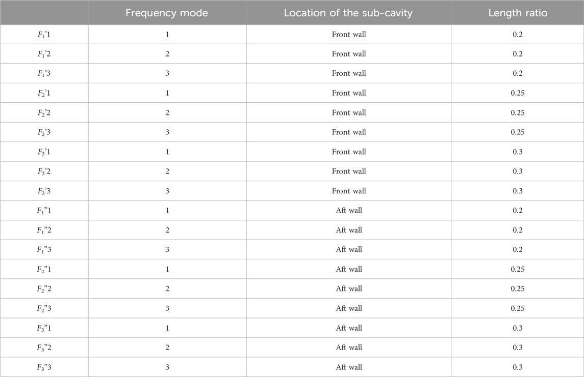
Table 1. Frequency Modes in different configurations.

3.1 Baseline cavity

Figure 6 shows the frequency spectrum for the baseline cavity. The spectrum shows three distinct peaks, with the dominant frequency at (F1) 7.2 kHz. The intensity of the oscillation, quantified by the power spectral density, obtained from the monitoring station of the probe at the aft wall is highest for all modes. This is the consequence of the vortices of the shear layer impinging over the trailing edge of the cavity and, thus, can be considered the origin of the disturbances in the flow field. F2 and F3 are the second and third modes of frequencies of 10.65 kHz and 18.64 kHz, respectively.

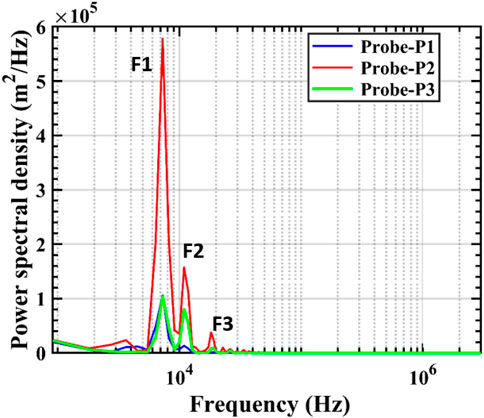
Figure 6. PSD vs. frequency plot in the confined cavity without the sub-cavity.

Figure 7A shows the flow feature (1). It is the shock generated at the ramp that causes the incoming flow to undergo deflection. This shock wave impinges on the shear layer, which has separated from the leading edge and travels towards the aft wall side of the cavity. A compression wave (3) is formed at the leading edge, as shown in Figure 7B. This wave is periodic, as initially reported by Heller and Bliss (1975)-Heller and Delfs (1996). It forms when an upstream traveling wave reaches the leading edge and bulges it (Figures 7A, G). A vortex (2) grows at the corner near the aft wall, as pointed out in Figure 7A. A pressure wave is, therefore, generated (Figures 7B–D). The generation of this pressure wave at the aft wall is also evident from the higher level of PSD value in the frequency spectrum of the baseline cavity. This wave amplifies while traveling upstream towards the front wall of the cavity. Figure 7D shows the pressure wave along with a wavefront (4), which trails with it. This wavefront also travels upstream but detaches from the internal pressure wave as it is about to reach the front wall of the cavity (Figures 7E–G). It, then, convects in the direction of the flow in the external medium Heller and Delfs (1996). It is a feature usual to a disturbance traveling at supersonic speeds. The angle of inclination of this wavefront is also dependent on the effective speed of flow inside the cavity. Moreover, this disturbance travels against the freestream with a higher effective Mach number. It is evident from Figures 7D, E, that the pressure waves reflect from the front wall of the cavity. This wave excites the shear layer while traveling back at the separation point. The shear layer bulges out (8) (Figure 7G) and then travels downstream to impinge on the trailing edge of the cavity. Therefore, a self-sustaining feedback loop exists inside a cavity and is well captured in this numerical simulation. The mass also scavenges out of the cavity through the trailing edge, marked as the features (9) and (10) in Figures 7H, I. This completes an entire oscillation cycle. The frequency of this oscillation is obtained in the spectrum as seen in Figure 6 with the dominant frequency at 7.2 kHz. The impinging of the shear layer and generation of the pressure waves at the aft wall of the cavity is also observed prominently in the contours.

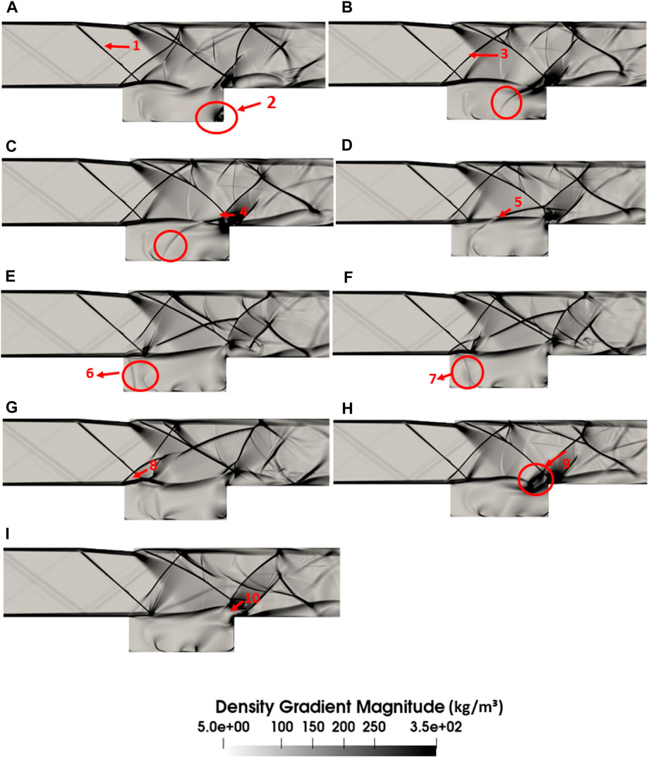
Figure 7. Numerical Schlieren of baseline supersonic cavity. The subfigures (A–I) illustrate the stages of a complete feedback cycle, from the initiation of upstream-traveling acoustic waves to the expulsion of mass from the cavity through the trailing edge.

We have mentioned in the article previously that we have used three monitoring points at the walls of the cavity for data collection. 8 shows the variation of pressure with time as recorded by probe 1 (at the front wall) and probe 2 (at the aft wall). The subfigure A of Figure 7 shows the generation of pressure waves at the aft wall, hence it corresponds to the highest pressure recorded at the aft wall. As the pressure wave travels upstream, the pressure at the aft wall decreases and at the last instance of the oscillation cycle which is shown in subfigure, I of 7 has the lowest pressure. The reverse happens in the front wall. The pressure wave requires some time to reach the front wall, hence, a lag is also seen between the data of the two probes in Figure 8.

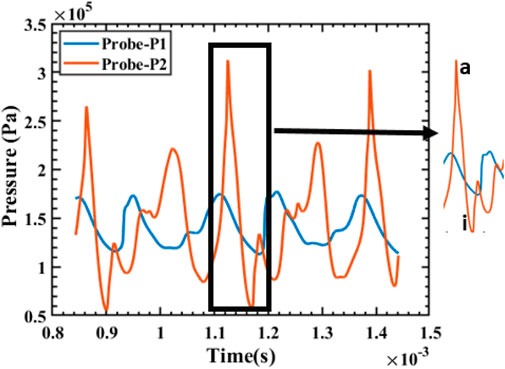
Figure 8. Variation of pressure with time in Probes one and two in the baseline cavity. Here, a and i correspond to the subfigures A and I of Figure 7.

The external flow is enclosed between the top wall of the confinement and the constant-pressure shear layer. Thereby, a shock train is formed in the domain. Figures 7C, D show interactions between the compression wave formed at the trailing edge and the reflected shock wave from the top wall.

3.2 Cavity with the front wall sub-cavity

Incorporating a front wall sub-cavity alters the frequencies as seen in Figure 9. The fundamental frequency is reduced to 2.9 kHz in the configuration when the sub-cavity length ratio is 0.2 (Figure 9A). This occurs due to the cessation of the feedback loop. This is also evident from the flow-field visualization in Figure 10. Here, F₁’2 and F₁’3 are the second and third harmonics of F₁’1, of frequencies 5.8 and 8.7 kHz respectively. The intensity of the fluctuations, which is inferred from the power spectral density is almost half in the presence of sub-cavity as compared to that obtained in its absence. When the sub-cavity length is increased to 0.25 (Figure 9B), the lower frequencies cease and two higher frequencies of 12.7 kHz (F₂’1) and 24.5 kHz (F₂’2) exist. On further increasing the length ratio to 0.3, a smaller frequency of 8.5 kHz (F₃’1) is observed (Figure 9C) alongside the higher frequencies at 12.7 kHz (F₃’2) and 24.5 kHz (F₃’3). Notably, the frequency of 12.7 kHz is dominant in both of these configurations. This frequency is related to the shear layer oscillation as there is a re-formation of the feedback loop (Figure 12). The intensity of the vibrations signified by the PSD is higher in these configurations than in the first configuration. The change in the dominant frequency with the change in the sub-cavity length ratio from 0.2 to 0.25 indicates a switch in the mode of oscillation.

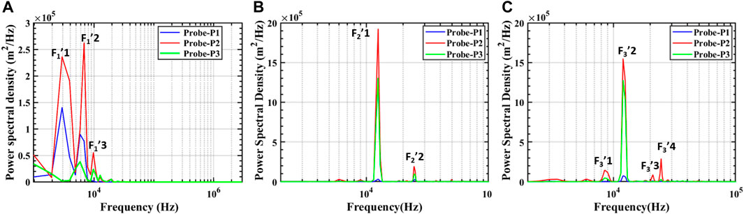
Figure 9. PSD vs. frequency plot in the confined cavity with a front wall sub-cavity of length ratio of (A) 0.2 (B) 0.25 (C) 0.3.

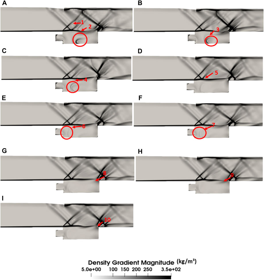
Figure 10. Numerical Schlieren of the frontwall subcavity of the length ratio of 0.2. The subfigures (A–I) illustrate the stages of a complete feedback cycle, from the initiation of upstream-traveling acoustic wave to its dissipation the expulsion of mass from the cavity through the trailing edge.

Figure 10 portrays the flow field and annotated features in the presence of a sub-cavity of length ratio 0.2 at the front wall. Figures 10A–C show the pressure wave (2) generated at the trailing edge traveling upstream towards the front wall. A vortex-like structure forms at the edge of the sub-cavity, which swirls, grows in size and interacts with the upstream traveling pressure wave (Figures 10B–F). The frequencies obtained in Figure 9A are related to this interaction phenomenon as there is no existence of the feedback loop. Post the interaction, the pressure wave dissipates. Unlike the cavity configuration without the sub-cavity, the pressure wave does not reach the front wall. Simultaneously, the shear layer grows and impinges on the trailing edge, unperturbed by the upstream traveling pressure wave. Hence, the feedback loop ceases to exist. There is an alternate inflow and outflow of mass, marked as (8)–(10) in Figures 10G–I.

Figure 11 shows the temporal pressure variation in the case of front wall sub-cavity of length ratio 0.2. Likewise in the case of the baseline cavity, the pressure is highest at the aft wall at instance ‘A’, which shows the generation of the pressure wave. With the convection of the pressure wave upstream, it slowly decreases to ‘I’. In this configuration, the pressure waves get dissipated, hence the rise in pressure as well as the lag in the data of the two probes are less.

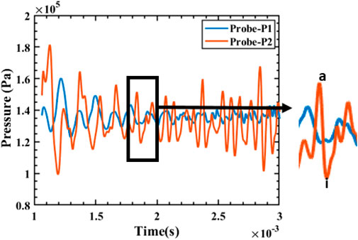
Figure 11. Variation of pressure with time in Probes one and two in the cavity with front wall sub-cavity of length ratio 0.2. Here, a and i correspond to the subfigures A and I of Figure 10.

The flow fields of the cavity with front wall sub-cavity of length ratios 0.25 and 0.3 are similar. Hence, to avoid redundancy, we have only presented the flow-field visualization of sub-cavity length ratio 0f 0.25. Figure 12 illustrates the variations in the flow field induced by the sub-cavity of lengths of 0.25. The pressure waves generated at the corner near the trailing edge travel upstream (as seen from subfigures A–C of Figure 12 to the leading edge. Subsequently, these waves enter the sub-cavity and get reflected from there to interact with the upstream traveling pressure wave of the next oscillation cycle (subfigures D–I). In contrast to the configuration with a sub-cavity length ratio of 0.2, the pressure waves in these configurations appear to stimulate the separating shear layer at the leading edge. The visible bulging of the shear layer in Figure 12 confirms the perturbation caused by the pressure waves. The feedback loop, therefore, exists in both configurations of the front wall sub-cavity length ratio of 0.25 and 0.3. However, unlike the baseline configuration, the reflection of the pressure waves takes place from the sub-cavity wall. The frequency of the shear layer oscillation is much higher than that present in the baseline configuration, as was seen in the frequency spectra of these configurations. Figure 13 shows the pressure at the probes at the front wall and aft wall varying with time. Similar to the previous cases, the highest pressure ‘A’ at the aft wall corresponds to the origin of the pressure wave and then decreases with its upstream convection to ‘I’. However, unlike the previous configurations, pressure at the front wall is also the highest at those instants. This implies that the time lag between the front and the aft walls reduces. We will focus on this reduction in time lag in our future studies.

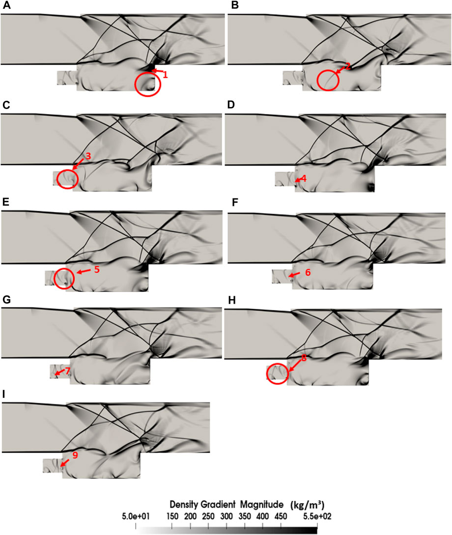
Figure 12. Numerical Schlieren of the front wall sub-cavity of the length ratio of 0.25. The subfigures (A–I) represent the different instants of a complete feedback cycle.

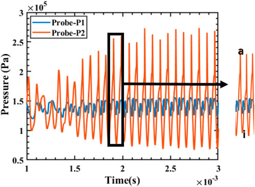
Figure 13. Variation of pressure with time in Probes one and two in the cavity with front wall sub-cavity of length ratio 0.25. Here, a and i correspond to the subfigures A and I of Figure 12.

3.3 Cavity with the aft wall sub-cavity

Figure 14 illustrates the impact of the placement of the sub-cavity at the aft wall. The frequency spectrum shows that when the sub-cavity length ratio is 0.2, the dominant frequency is 6.7 kHz (F₁″1), while other frequencies remain imperceptible. As the length of the sub-cavity increases, a lower frequency at 3.298 kHz (F₂″1 and F₃″1) is also seen in the spectrum. This fundamental frequency is accompanied by harmonics at 6 kHz (F₂″2 and F₃″2), 9.3 kHz (F₂″3 and F₃″3), and 12.09 kHz (F₂″4 and F₃″4). The alteration of the length of the sub-cavity at the aft wall influences the intensity of the oscillations, as evident from the PSD values. The frequency of 6.7 kHz is dominant in the case of the sub-cavity length ratio of 0.2, while an increase in the length of the sub-cavity results in the fourth mode at 12.09 kHz as the dominant frequency, which indicates the switch in mode due to the change in length of the sub-cavity. The occurrence of such frequencies is understood clearly from the flow-field visualization in Figure 15.Regardless of the length ratio, the density gradient contours of the sub-cavities placed at the aft wall, depict a consistent flow field. This is also evident from the frequency spectra of these configurations. Therefore, the numerical schlieren of the sub-cavity length ratio of 0.2 at the aft wall is presented in this article for brevity (Figure 15). In the first three sub-figures (A–C), a periodic inflow and outflow of mass from the aft wall generate a wave. This wave expands, grows, and impinges on the cavity floor (subfigures D–F). Subsequently, it gets dissipated without reaching the leading edge (subfigures G–I). The next cycle of oscillation commences after that. The frequency in the spectrum seen in Figure 14 is attributed to this wave, as there is no indication of the excitement of the shear layer by the pressure wave. The shear layer is almost parallel to the freestream flow and is not deformed by the pressure waves, as in the case of the baseline cavity. Hence, the sub-cavities at the aft wall disrupt the feedback loop. The shear layer separates, moves downstream, and impinges on the aft wall, a characteristic of deep cavities. Although the feedback loop ceases to exist in the aft wall sub-cavity configuration, the dominant frequency obtained in the presence of the aft wall sub-cavity length of 0.2 is 6 kHz, which is higher than its front wall counterpart.

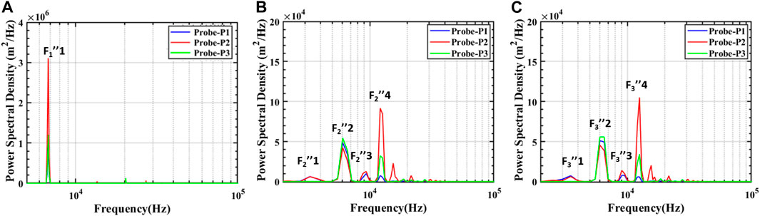
Figure 14. PSD vs. frequency plot in the confined cavity with an aft wall sub-cavity of length ratio of (A) 0.2 (B) 0.25 (C) 0.3.

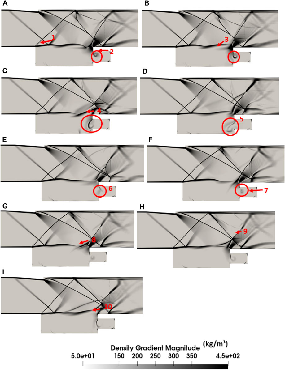
Figure 15. Numerical Schileren of the aft wall sub-cavity of the length ratio of 0.2. The subfigures (A–I) show different instants of a complete feedback cycle, generation of the acoustic wave, its oscillation, dissipation and expulsion of mass through the trailing edge.

In Figure 16, we see the variation of pressure obtained by the front wall and the aft wall probes with time. Similar to the other configurations, the highest pressure at the aft wall is at ‘A’, when the pressure waves get generated. In the aft wall sub-cavities, the pressure waves grow and oscillate in the sub-cavity itself and then dissipate before the onset of the next cycle. This is shown by ‘I’ in both Figures 15, 16. The plot also shows that the pressure is considerable in the front wall. From the numerical schlieren (Figure 15), we see that the pressure waves have not reached the front wall. So, this pressure recorded at the front wall probe can correspond to the shear layer. However, we need further study to understand this occurrence.

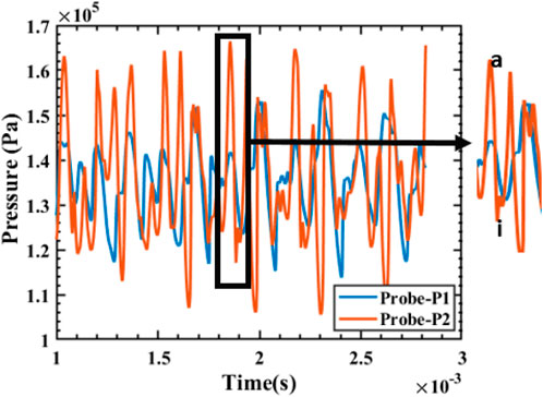
Figure 16. Variation of pressure with time in Probes one and two in the cavity with aft wall sub-cavity of length ratio 0.2. Here, a and i correspond to the subfigures A and I of Figure 15.

We can infer from the above preliminary spectral analysis and the numerical flow field visualization that the front wall sub-cavity of length, 0.2 times the cavity length, and all the aft wall sub-cavity configurations effectively disrupt the feedback loop and hence, reduce the oscillation of the separating shear layer. The variation of the normalized mean pressure along the cavity walls in the three configurations of the baseline cavity and sub-cavities of length ratio 0.2 at the front and the aft walls also justify our findings (Figure 17). However, reduced order modeling like the Proper Orthogonal Decomposition (POD) and Dynamic Mode Decomposition (DMD), will aid in a better understanding of the frequency obtained in the spectra of all the configurations and their corresponding flow structures. This analysis requires a three-dimensional study of the configurations, which is the scope of our future study.

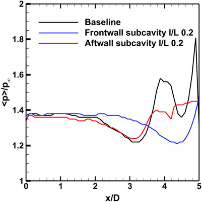
Figure 17. Variation of normalized time-averaged pressure at the cavity walls at different configurations.

4 Conclusion

The numerical study investigates the flow fields of a supersonic cavity with and without sub-cavity, placed in a confined passage at a freestream Mach number of 1.71. It employs an explicit finite volume density-based solver in the OpenFOAM framework. The solver is initially validated using the most economical grid by comparing the time-averaged pressure along the cavity wall against the experimental data provided by Gruber et al. (2001). Excellent agreement is obtained, and thus, further analysis is performed for a supersonic cavity placed inside a confined passage. Density gradient magnitude contours are utilized to understand the associated flow features. The pressure fluctuations obtained from different monitoring stations or probe locations in the domain are analyzed using PSD analysis to filter out the relevant frequencies. The numerical Schileren obtained from the gradient of the density in space is then used to understand the corresponding flow structures. The numerical simulations provide the following key highlights of this article:

• PSD analysis shows that the front wall sub-cavity length ratio of 0.2 reduces the dominant frequency of the oscillations inside the cavity by nearly 60%. It also reduces the intensity of the oscillations. The density gradient magnitude contours establish that the separating shear layer at the leading edge is not affected by the flow features inside the cavity when the sub-cavity is present at the front wall. The pressure waves interact with the vortices that originate at the edge of the sub-cavity. Instead of reflecting, these waves dissipate. Hence, the feedback loop gets disrupted in the presence of this sub-cavity.

• Increasing the length of the sub-cavity at the front wall increases the dominant frequency, and the shear layer is perturbed to a greater extent by the upstream traveling pressure waves. The feedback loop is therefore established.

• The numerical schlieren, shows that when the sub-cavities are present at the aft wall, the pressure wave generated gets dissipated before reaching the leading edge. Therefore, the shear layer remains unperturbed by the wave. The feedback loop ceases to exist in the case of all the sub-cavities at the aft wall. Analysis infers that the sub-cavity at the aft wall of length ratio 0.2 reduces the dominant frequency by 7%, whereas when the sub-cavity to main cavity length ratios are between 0.25 and 0.3, the dominant frequency is the fourth mode, which is more than that of the baseline cavity.

The present study indicates that, with a constant length-to-depth ratio and freestream conditions, increasing the length of the front wall sub-cavity intensifies the cavity oscillations. The feedback loop is ceased in the front wall sub-cavity with a length ratio of 0.2 and all the aft wall sub-cavities. The highest suppression of fluctuations is obtained at a sub-cavity length ratio of 0.2 at the midpoint of the front wall. It is crucial to note that the present investigation utilizes k-ω SST for the turbulence modeling. A more detailed analysis of the fine-scale turbulence using the three-dimensional Large Eddy Simulation (LES) for turbulence modeling is plausible. The study’s forthcoming phase will explore the impact of flow Mach numbers within the enclosed passage and the positioning of the sub-cavity at the wall, thereby assessing their roles in sub-cavity control mechanisms. Additionally, reduced-order modeling will be employed to gain deeper insights into the frequencies obtained in the spectral analysis.

Data availability statement

The raw data supporting the conclusion of this article will be made available by the authors, without undue reservation.

Author contributions

SB: Conceptualization, Data curation, Formal Analysis, Investigation, Software, Validation, Visualization, Writing–original draft, Writing–review and editing. AR: Investigation, Methodology, Software, Visualization, Writing–review and editing. AD: Conceptualization, Funding acquisition, Project administration, Resources, Supervision, Writing–review and editing. MS: Resources, Supervision, Writing–review and editing.

Funding

The author(s) declare that no financial support was received for the research, authorship, and/or publication of this article.

Acknowledgments

The authors would like to acknowledge the National Supercomputing Mission (NSM) for providing computing resources of “Param Sanganak” at IIT Kanpur, which is implemented by CDAC and supported by the Ministry of Electronics and Information Technology (MeitY) and the Department of Science and Technology (DST), Government of India. We would like to acknowledge the IIT-K Computer Centre (www.iitk.ac.in/cc) for providing the resources to perform the computation work. This support is gratefully acknowledged.

Conflict of interest

The authors declare that the research was conducted in the absence of any commercial or financial relationships that could be construed as a potential conflict of interest.

Publisher’s note

All claims expressed in this article are solely those of the authors and do not necessarily represent those of their affiliated organizations, or those of the publisher, the editors and the reviewers. Any product that may be evaluated in this article, or claim that may be made by its manufacturer, is not guaranteed or endorsed by the publisher.

References

Abdolahipour, S. (2023). Effects of low and high frequency actuation on aerodynamic performance of a supercritical airfoil. Front. Mech. Eng. 9, 1290074. doi:10.3389/fmech.2023.1290074
Abdolahipour, S., Mani, M., and Shams Taleghani, A. (2022a). Experimental investigation of flow control on a high-lift wing using modulated pulse jet vortex generator. J. Aerosp. Eng. 35, 05022001. doi:10.1061/(asce)as.1943-5525.0001463
Abdolahipour, S., Mani, M., and Shams Taleghani, A. (2022b). Pressure improvement on a supercritical high-lift wing using simple and modulated pulse jet vortex generator. Flow, Turbul. Combust. 109, 65–100. doi:10.1007/s10494-022-00327-9
Abdolahipour, S., Mani, M., and Taleghani, A. S. (2021). Parametric study of a frequency-modulated pulse jet by measurements of flow characteristics. Phys. Scr. 96, 125012. doi:10.1088/1402-4896/ac2bdf
Alam, M. M., Matsuob, S., Teramotob, K., Setoguchib, T., and Kim, H.-D. (2007). A new method of controlling cavity-induced pressure oscillations using sub-cavity. J. Mech. Sci. Technol. 21, 1398–1407. doi:10.1007/bf03177426
Azadi, S., Abjadi, A., Vahdat Azad, A., Ahmadi Danesh Ashtiani, H., and Afshar, H. (2023). Enhancement of heat transfer in heat sink under the effect of a magnetic field and an impingement jet. Front. Mech. Eng. 9, 1266729. doi:10.3389/fmech.2023.1266729
Chakravarthy, R., Nair, V., Muruganandam, T., and Ghosh, S. (2018). Analytical and numerical study of normal shock response in a uniform duct. Phys. Fluids 30. doi:10.1063/1.5027903
Chavan, T., Chakraborty, M., and Vaidyanathan, A. (2022). Experimental and modal decomposition studies on cavities in supersonic flow. Exp. Therm. Fluid Sci. 135, 110600. doi:10.1016/j.expthermflusci.2022.110600
Devaraj, M. K. K., Jutur, P., Rao, S., Jagadeesh, G., and Anavardham, G. T. (2020). Experimental investigation of unstart dynamics driven by subsonic spillage in a hypersonic scramjet intake at mach 6. Phys. Fluids 32. doi:10.1063/1.5135096
Emmert, T., Lafon, P., and Bailly, C. (2009). Numerical study of self-induced transonic flow oscillations behind a sudden duct enlargement. Phys. fluids 21. doi:10.1063/1.3247158
Gruber, M., Baurle, R., Mathur, T., and Hsu, K.-Y. (2001). Fundamental studies of cavity-based flameholder concepts for supersonic combustors. J. Propuls. power 17, 146–153. doi:10.2514/2.5720
Heller, H., and Bliss, D. (1975). “The physical mechanism of flow-induced pressure fluctuations in cavities and concepts for their suppression,” in 2nd Aeroacoustics conference, 491.
Heller, H., and Delfs, J. (1996). Cavity pressure oscillations: the generating mechanism visualized. Lett. Ed. im J. Sound Vib. 196 (2), 248–252. doi:10.1006/jsvi.1996.0480
Heller, H. H., Holmes, D., and Covert, E. E. (1971). Flow-induced pressure oscillations in shallow cavities. J. sound Vib. 18, 545–553. doi:10.1016/0022-460x(71)90105-2
Jain, P., Sekar, A., and Vaidyanathan, A. (2023). Effects of multiple subcavities with floor subcavity in supersonic cavity flow. Propuls. Power Res. 12, 114–137. doi:10.1016/j.jppr.2023.02.003
Jain, P., and Vaidyanathan, A. (2021). Aero-acoustic feedback mechanisms in supersonic cavity flow with subcavity. Phys. Fluids 33. doi:10.1063/5.0066694
Johnson, A. D., and Papamoschou, D. (2010). Instability of shock-induced nozzle flow separation. Phys. Fluids 22. doi:10.1063/1.3278523
Karthick, S. (2021). Shock and shear layer interactions in a confined supersonic cavity flow. Phys. Fluids 33. doi:10.1063/5.0050822
Krishnamurty, K. (1955) Acoustic radiation from two-dimensional rectangular cutouts in aerodynamic surfaces. Tech. rep.
Lad, K. A., Vinil Kumar, R., and Vaidyanathan, A. (2018). Experimental study of subcavity in supersonic cavity flow. AIAA J. 56, 1965–1977. doi:10.2514/1.j056361
Lawson, S., and Barakos, G. (2011). Review of numerical simulations for high-speed, turbulent cavity flows. Prog. Aerosp. Sci. 47, 186–216. doi:10.1016/j.paerosci.2010.11.002
Lee, Y., Kang, M., Kim, H., and Setoguchi, T. (2008). Passive control techniques to alleviate supersonic cavity flow oscillation. J. Propuls. Power 24, 697–703. doi:10.2514/1.30292
Malhotra, A., and Vaidyanathan, A. (2016). Aft wall offset effects on open cavities in confined supersonic flow. Exp. Therm. Fluid Sci. 74, 411–428. doi:10.1016/j.expthermflusci.2015.12.015
Menter, F., Kuntz, M., and Bender, R. (2003). “A scale-adaptive simulation model for turbulent flow predictions,” in 41st aerospace sciences meeting and exhibit, 767.
Modesti, D., and Pirozzoli, S. (2017). A low-dissipative solver for turbulent compressible flows on unstructured meshes, with openfoam implementation. Comput. Fluids 152, 14–23. doi:10.1016/j.compfluid.2017.04.012
Noori, M. S., Taleghani, A. S., and Rahni, M. T. (2021). Surface acoustic waves as control actuator for drop removal from solid surface. Fluid Dyn. Res. 53, 045503. doi:10.1088/1873-7005/ac12af
Plentovich, E. B., Stallings Jr, R. L., and Tracy, M. B. (1993) Experimental cavity pressure measurements at subsonic and transonic speeds. Static-pressure results. Tech. rep.
Rahni, M. T., Taleghani, A. S., Sheikholeslam, M., and Ahmadi, G. (2022). Computational simulation of water removal from a flat plate, using surface acoustic waves. Wave Motion 111, 102867. doi:10.1016/j.wavemoti.2021.102867
Rossiter, J. (1964). Wind-tunnel experiments on the flow over rectangular cavities at subsonic and transonic speeds.
Rowley, C. W., and Williams, D. R. (2006). Dynamics and control of high-Reynolds-number flow over open cavities. Annu. Rev. Fluid Mech. 38, 251–276. doi:10.1146/annurev.fluid.38.050304.092057
Sahoo, N., Kulkarni, V., Saravanan, S., Jagadeesh, G., and Reddy, K. (2005). Film cooling effectiveness on a large angle blunt cone flying at hypersonic speed. Phys. Fluids 17. doi:10.1063/1.1862261
Saravanan, R., Desikan, S., and Tm, M. (2020). Isolator characteristics under steady and oscillatory back pressures. Phys. Fluids 32, 096104. doi:10.1063/5.0016360
Sekar, K. R., Karthick, S., Jegadheeswaran, S., and Kannan, R. (2020). On the unsteady throttling dynamics and scaling analysis in a typical hypersonic inlet–isolator flow. Phys. Fluids 32. doi:10.1063/5.0032740
Stallings, R. L., and Wilcox, F. J. (1987) Experimental cavity pressure distributions at supersonic speeds. Tech. rep.
Taleghani, A. S., Shadaram, A., Mirzaei, M., and Abdolahipour, S. (2018). Parametric study of a plasma actuator at unsteady actuation by measurements of the induced flow velocity for flow control. J. Braz. Soc. Mech. Sci. Eng. 40, 173–213. doi:10.1007/s40430-018-1120-x
Tracy, M. B. (1992) Measurements of fluctuating pressure in a rectangular cavity in transonic flow at high Reynolds numbers, 4363. Edinburgh Gate, Harlow England: National Aeronautics and Space Administration, Office of Management.
Versteeg, H. K., and Malalasekera, W. (2007) An introduction to computational fluid dynamics: the finite volume method. Edinburgh Gate, Harlow England: Pearson education.
Vikramaditya, N., and Kurian, J. (2009). Pressure oscillations from cavities with ramp. AIAA J. 47, 2974–2984. doi:10.2514/1.43068
Woolley, J. P., and Karamcheti, K. (1974). Role of jet stability in edgetone generation. AIAA J. 12, 1457–1458. doi:10.2514/3.49525
Yilmaz, I., and Aradag, S. (2013). Numerical laser energy deposition on supersonic cavity flow and sensor placement strategies to control the flow. Sci. World J. 2013, 1–8. doi:10.1155/2013/141342
Keywords: cavity, sub-cavity, flow control mechanism, feedback loop, power spectral density
Citation: Bhaduri S, Ray A, De A and Sugarno MI (2024) Flow control in a confined supersonic cavity flow using subcavity. Front. Mech. Eng 10:1378433. doi: 10.3389/fmech.2024.1378433
Received: 29 January 2024; Accepted: 08 May 2024;
Published: 30 May 2024.
Edited by:
Santanu Ghosh, Indian Institute of Technology Madras, IndiaReviewed by:
Arash Shams Taleghani, Ministry of Science, Research and Technology, IranSoheila Abdolahipour, Aerospace Research Institute, Iran
Copyright © 2024 Bhaduri, Ray, De and Sugarno. This is an open-access article distributed under the terms of the Creative Commons Attribution License (CC BY). The use, distribution or reproduction in other forums is permitted, provided the original author(s) and the copyright owner(s) are credited and that the original publication in this journal is cited, in accordance with accepted academic practice. No use, distribution or reproduction is permitted which does not comply with these terms.
*Correspondence: Ashoke De, ashoke@iitk.ac.in