Research on Ferromagnetic Hysteresis of a Magnetorheological Fluid Damper

Introduction

Magnetorheological (MR) dampers have the advantages of continuous adjustable damping force, large and wide adjustable range, low energy consumption and wide dynamic range. Magnetorheological dampers have attracted wide attention in the field of Engineering Vibration reduction. Relevant research has been widely carried out in vehicle, civil engineering, household appliances, medical health, military engineering and other fields (Ahmadian et al., 2002; Carlson, 2002; Hiemenz et al., 2009; Gordaninejad et al., 2010). In recent years, the research results of MR dampers have gradually penetrated into the field of shock buffer control (Singh et al., 2014; Shou et al., 2018; Li et al., 2019). It provides a new way of thinking for shock cushioning in engineering. However, the inherent hysteretic non-linearity of MR dampers is one of the main reasons that limit their wide application in engineering, especially in the field of shock buffering. The hysteretic non-linearity of MR dampers is particularly prominent because the shock buffering system requires rapid and accurate response control to achieve impact resistance.

The hysteretic non-linearity of MR dampers mainly comes from two aspects (Seong et al., 2009):

(1) Hysteretic non-linearity between damping force and velocity. This part of the hysteresis is caused by friction and fluid compression in the damper, as well as the non-linear rheological properties of magnetorheological fluid, such as yield stress and shear thinning. Hysteretic non-linearity between damping force and velocity can usually be described and eliminated by establishing hysteretic dynamic model.

(2) Hysteresis non-linearity (i.e., hysteresis characteristics) between adjustable damping force and control current. It is caused by the inclusion of ferromagnetic materials in the internal structure of MR damper. The hysteresis non-linearity between magnetic induction and magnetic field intensity is caused by the magnetization characteristics of ferromagnetic materials, which is commonly called hysteresis loop. The magnetic field intensity of the internal damping channel of MR damper is generated by the control current. The adjustable yield stress is a function of magnetic induction intensity. Therefore, the hysteretic non-linearity between magnetic induction and magnetic field intensity will greatly affect the relationship between damping force and control current.

On the one hand, most low-speed vibration systems do not require high real-time performance, so the hysteretic non-linearity between the adjustable damping force and the control current of MR dampers has little effect. For a long time, hysteresis non-linearity has not attracted enough attention. On the other hand, it is difficult to model this part of hysteresis with dynamic equation of the MR damper, so it is ignored by most researchers.

However, the magnetorheological materials and structures in shock buffer systems are greatly affected by the coupling of magnetic field, flow field, temperature field and other physical fields. The structural parameters of MR dampers change with time, which are unknown, time-varying and non-linear. This makes the hysteretic non-linearity between the adjustable resistance and current of MR dampers complicated and uncertain. For shock buffering system, the hysteresis characteristics of MR dampers greatly affect the accuracy of prediction and control of damping force. The hysteresis characteristics of MR dampers for impact buffering are tested experimentally and the model is established in this paper, which will provide a research basis for the compensation or elimination of the hysteresis of MR fluid dampers.

At present, there are three most commonly used methods for hysteresis modeling: Preisach hysteresis model, J-A hysteresis model and neural network hysteresis model. Preisach model is the most general operator-based model. It assumes that hysteresis can be modeled as the sum of a weighted hysteresis operator. However, the construction of weighting function and the experimental measurement of related parameters are more difficult, and the repeatability of a large number of data points and system behavior has a direct impact on the accuracy of the model (Joseph, 2001). On the other hand, the establishment of Preisach model needs to take into account the anisotropy and frequency factors (Ge and Jouaneh, 1997), which leads to a much too complication mathematical expression, so it is not convenient for numerical calculation. Neural network model has strong non-linear fitting ability, so it can map almost any complex non-linear relationship. At the same time, it has strong robustness, memory ability, non-linear mapping ability and strong self-learning ability. However, the approximation and generalization ability of network models are closely related to the typicality of learning samples, and neural network methods usually require at least thousands or even millions of labeled samples. It is difficult to select typical samples from the problem to form training set.

J-A mathematical model was presented by Jiles D C and Atherton D L to descript the hysteresis mechanism in ferromagnets (Jiles and Atherton, 1986). J-A hysteresis model is a typical differential equation-based model (Jiles and Atherton, 1986, 1998). It is based on the domain wall theory of ferromagnetic materials. J-A model theory holds that the existence of non-magnetic inclusions, internal stresses, grain boundaries, and other constraints hinders the irreversible magnetization process caused by domain wall substitution, resulting in hysteresis. This explanation accords with the physical law of hysteresis phenomenon. Moreover, J-A model has fewer parameters, and its physical meaning is clear and easy to implement. This model can truly describe the non-linear relationship between magnetic field intensity and magnetic induction intensity. The accurate hysteresis loop can be obtained by solving the differential equation of J-A model. Therefore, J-A model is widely used in the field of hysteresis modeling and simulation of ferromagnetic materials. In this paper, the magnetic circuit part of the MR fluid damper is composed of piston, cylinder and MR fluid. The materials of the piston and the cylinder of the MR fluid damper in this paper are both SAE1045 steel. And the MR fluid contains soft magnetic particles. Therefore, it is reasonable to use J-A model to descript the ferromagnetic hysteresis curve of the MR fluid damper.

Because of the complexity of hysteresis non-linearity, the calculation of model parameters is a key problem in the process of establishing J-A hysteresis model. Many non-linear optimization methods are used to calculate the parameters of J-A hysteresis model. However, these optimization methods are vulnerable to the selection of initial values of parameters. For example, Jiles and Thoelke proposed a classical algorithm to estimate the parameters of J-A model (Jiles et al., 1992). By iterating the parameters, they find the optimal combination of parameters. However, the initial values of the parameters and the iteration order of the parameters have great influence on the method, which leads to low identification accuracy. In recent years, many intelligent optimization algorithms have been developed rapidly, and have been increasingly introduced into J-A model parameter identification, including particle swarm optimization, genetic algorithm, and neural network (Wilson et al., 2001; Salvini and Fulginei, 2002; Cao et al., 2004; Leite et al., 2004; Marion et al., 2008; Trapanese, 2011).

In this paper, the J-A model is used to describe the hysteresis non-linearity between the magnetic induction intensity and the current of the MR fluid damper for shock buffering. The J-A hysteresis model is simulated numerically. The hysteresis characteristics of MR fluid damper damping channel are obtained by embedding small size Hall sensors into the damping channels. Five parameters of J-A hysteresis model are identified by the particle swarm optimization.

Theory of Jiles-Atherton Model

J-A model theory assumes that domains with the same orientation belong to the same magnetic phase. Therefore, the spatial distribution of magnetic domains with different orientations need not be considered. It can only be regarded as the thermodynamic statistical distribution of many domains with different orientations. At the same time, it is assumed that the angle of domain wall is 180 degrees, and the thickness of domain wall is not taken into account. In addition, it is assumed that all pinning points are uniformly distributed and have the same pinning energy (Jiles and Atherton, 1986). It is assumed that the irreversible magnetization component caused by domain wall substitution in J-A model is M_irr. The reversible magnetization component caused by domain wall bending is M_rev. So the total magnetization is

where M_irr and M_rev can be obtained from the hysteresis-free intensity of magnetization M_an.

where c is a reversible magnetization coefficient. It characterizes the relationship between the reversible and irreversible components of magnetization.

Weiss's “molecular field” theory holds that there exists a strong field effect in ferromagnetic materials. Under this effect, the magnetic moments of each atom tend to align spontaneously and produce spontaneous magnetization until saturation. Weiss calls this action a “molecular field” and expresses it in H_m. The expression is shown as,

where α is the coefficient of the molecular field. According to Weiss molecular field theory, α can be expressed as $\alpha =\frac{\theta }{C}$, where θ is paramagnetic Curie temperature, and C is the Curie constant.

Assuming that the direction of the external magnetic field H is the same as that of the magnetization intensity M, the effective magnetic field strength is

The hysteresis-free magnetization M_an is described by an improved Langevin function shown as

where M_s is the saturated magnetization density. It is related to the material's own characteristics and temperature. a is a shape parameter of non-hysteresis magnetization curve.

The magnetization intensity M can be obtained by Equation (1) and (2).

The following equation is obtained by the derivation of external magnetic field H on both sides of Equation (6).

The differentiation of magnetic field strength H by irreversible component M_irr is expressed by the following equation

where k is the constraint parameter. It is multiplied by vacuum permeability μ₀ as hysteresis loss parameter K. K represents the change of energy loss in each element during magnetization, which is proportional to the number of pinning points and energy. δ is a parameter indicating the direction of magnetic field change. When dH/dt > 0, δ = 1. When dH/dt < 0, δ = −1.

The following equation is obtained by Equation (7) and (8)

or

Simulation of Jiles-Atherton Model

Jiles-Atherton model describes the relationship between magnetization intensity M and magnetic field H. Because the magnetic induction intensity B is directly involved in the calculation of the electromagnetic energy conversion relationship of the MR fluid damper, the differential equation of M-H is transformed to obtain the B-H differential relationship as follows

where, ${\mu }_0=4\pi \times 10^{-7}N/A^2$ is the vacuum permeability.

During the operation of MR fluid damper, the magnetic field strength H is determined by the current I loaded in the electromagnetic coil. The relationship between H and I is

where H is the intensity of the magnetic field, N is the number of turns of the excitation coil, I is the excitation current and Le is the effective length of the magnetic circuit.

Thus, the relationship between M-H can be transformed to B-I. In order to facilitate the numerical simulation, the two sides of Equation (8) are multiplied by dH/dt simultaneously and Equation (8) is transformed into a differential of time, as shown in the following formula.

Equation (11), (12), and (13) is transformed into differential equation with current as input and magnetic induction as output. Then the hysteresis model is established by using the simulation software MATLAB/SIMULINK. The simulation model is shown in Figure 1. Given five parameters of J-A hysteresis model (M_s, a, α, c, k), the hysteresis curve between magnetic induction intensity and current can be obtained. Figure 2 is the hysteresis loop between magnetic induction B and current I when $M_s=1.6\times 10^6$, a = 1,100, α = 0.0017, c = 0.26, k = 400.

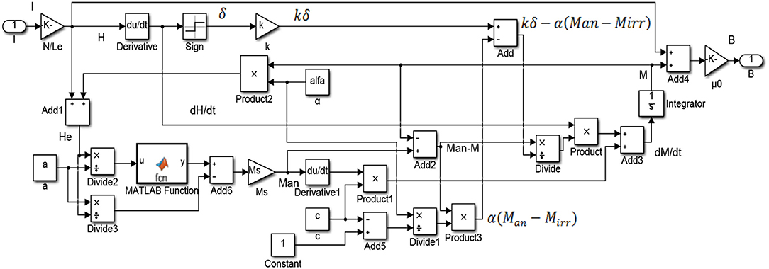
Figure 1. Implementation of Jiles-Atherton model by SIMULINK.

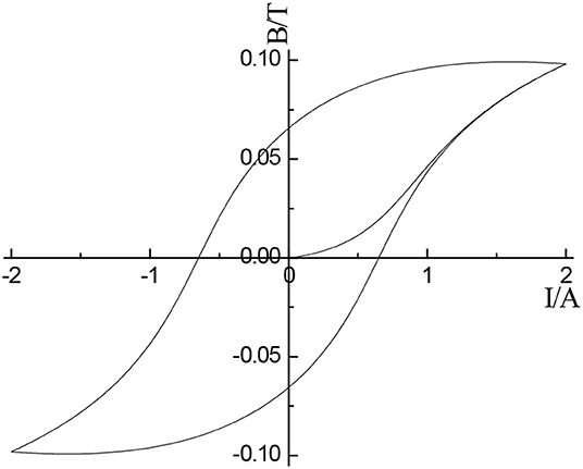
Figure 2. J-A hysteresis loop by numerical simulation ($M_s=1.6\times 10^6$, a = 1,100, α = 0.0017, c = 0.26, k = 400).

Testing of Hysteresis Characteristics of MR Fluid Damper

The hysteresis characteristic test system of MR fluid damper designed in this paper is shown in Figure 3. The test system consists of DC power supply, MR fluid damper embedded in Hall sensors, PXI data acquisition system, LabVIEW test interface and 3.3 voltage power supply circuit board. The hardware of data acquisition system adopts PXIe-6363 module of PXI acquisition system produced by National Instruments Corporation. The test interface software is programmed by LabVIEW. The Hall sensors A1304ELHLX-05-T produced by Allegro Micro Systems is used in this paper. In order to measure the magnetic induction intensity of MR fluid passing vertically through the damping channel, two Hall sensors are embedded in the MR fluid damper and installed, respectively, on the circumferential surface of the two stages of the piston of the MR fluid damper. According to the structure of MR fluid damper, the circumferential area of the installation position of the second sensor is twice the circumferential area of the installation position of the first sensor. Every Hall sensor chip has three pins, which are 3.3 voltage power supply terminal, grounding terminal and output terminal, respectively. The power supply terminal and the ground terminal are connected to the power supply circuit board. The output terminal and the ground terminal are connected to the data acquisition module. According to the static output voltage and sensitivity coefficient of the sensor, the corresponding magnetic induction intensity is converted by the test interface software designed by LabVIEW. The DC power supplies current to the coil of MR fluid damper. The LabVIEW test interface software not only controls the acquisition hardware but also realizes the functions of saving experimental data and drawing and displaying hysteresis loop curve.

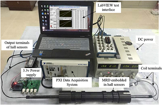
Figure 3. Experimental setup of hysteresis characteristics of MR fluid damper.

Figure 4 shows the exact locations and installation of the two Hall sensors and the installation position of the two coils. The two Hall sensors are installed on the surfaces of the circumferences of the piston of the MR fluid damper. In order to paste the two sensors on the surfaces tightly, the installed positions should be smoothed by a file before installation. As shown in Figure 4, the circumferential area where hall sensor 2 installed (area 2) is twice of the circumferential area where hall sensor 1 installed (area 1).

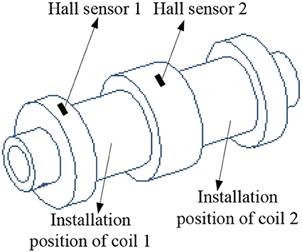
Figure 4. The sketch of the piston of the MR fluid damper labeled the locations and installation of the two Hall sensors.

The hysteresis characteristics of the MR fluid damper for shock buffering are tested by using the experimental setup shown in Figure 3. The measurement of magnetic flux density is under the work of coil 1. The experimental scheme is to change the output current of DC power supply from 0 to 2 A. A total of 27 current values were selected to apply on the coils of the MR fluid damper. Then from 2 to 0 A, the corresponding 27 current values are also applied on the coils. The applied currents and the output voltage values of Hall sensor in the whole two processes are acquired by PXI data acquisition system. After a group of testing, the hysteresis curve is automatically drawn by the LabVIEW test interface. The test interface implemented by LabVIEW is shown in Figure 5. Figure 6 are the hysteresis characteristic curves measured by different Hall sensor on different stage of the piston of the MR fluid damper, respectively.

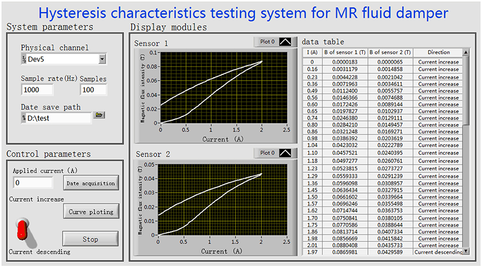
Figure 5. Interface of hysteresis testing system for MR fluid damper utilizing LabVIEW.

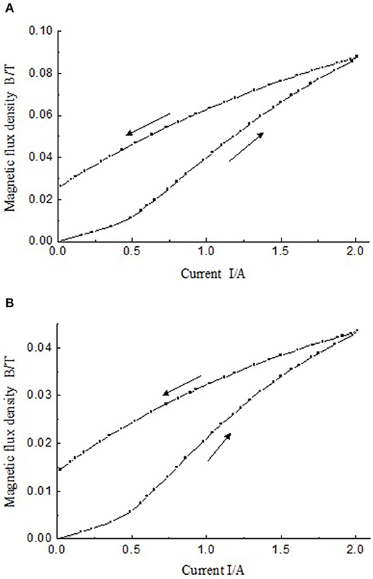
Figure 6. Magnetic hysteresis curves measured by the sensors installed on circular surfaces of the piston of the MR fluid damper. (A) First sensor; (B) Second sensor.

As can be seen from Figure 6, the magnetic flux intensity increases with the increase of the current. According to Kirchhoff's First Law of magnetic circuit, the magnetic flux density of area 1 theoretically is twice of that of area 2. Figure 6 shows that the maximum magnetic flux density measured by sensor 1 is around 0.09 Tesla and the maximum magnetic flux density measured by sensor 2 is around 0.045 Tesla. The results are consistent with Kirchhoff's First Law of magnetic circuit. These results are consistent with the theoretical analysis. In the descending phase of current, the value of magnetic induction does not decrease to 0 with the input current being 0. The values measured by the two sensors are 0.026 and 0.015 tesla, respectively. The curve of magnetic flux intensity changing with current shows obvious hysteresis characteristics. The measured curves in Figures 6A,B show obvious hysteresis characteristic which is consistent with the J-A hysteresis loop by simulation shown in Figure 2.

Parameter Identification of Jiles-Atherton Model

Theory of Particle Swarm Optimization

Particle swarm optimization (PSO) is an intelligent optimization algorithm derived from the study of bird predation behavior. This algorithm was first proposed by American electrical engineer Eberhart and social psychologist Kennedy in 1995 (Kennedy, 2011). The quality of PSO solution is evaluated by fitness. It has no “crossover” and “mutation” operations of genetic algorithm, so its structure is simpler. In addition, PSO algorithm benefits from individual cooperation and information sharing to find the optimal solution. This algorithm has the advantages of easy implementation, less adjustment parameters and strong global optimization ability. PSO algorithm is widely used in the fields of electrical engineering, robot, and medical field (Yoshida et al., 2001; Bingul and Karahan, 2011; Hsieh et al., 2014).

Initialization of PSO algorithm generates a group of particles (random solutions) randomly, and the characteristics of particles are represented by three parameters: position, velocity, and fitness. The fitness value is calculated by fitness function. Whether it is good or not indicates the good or bad of particles. During the iteration, each particle moves in the search space. They update individual location by tracking individual extreme value and group extreme value. The individual extreme value P_best and the population extreme value G_best refer to the fitness value of the location experienced by the individual and the fitness value of the optimal location searched by all the particles in the population, respectively. The fitness value is calculated once the particle updates its position. After each update, the fitness and individual extremum of the new particle and the group extremum are compared, so that the position of individual extremum and group extremum is updated continuously.

Assume that the position and velocity of a particle are recorded as X_i and V_i, respectively. Assuming that the search space of the problem is a D-dimensional space, the position and velocity of particles can be expressed as X_i = [x_i1, x_i2, ⋯ , x_id] and V_i = [v_i1, v_i2, ⋯ , v_id]. The individual extremum of the particle is denoted as P_i = [p_i1, p_i2, ⋯ , p_id]. The extremum of the whole population is denoted as P_g = [p_g1, p_g2, ⋯ , p_gd]. The velocity and the position of particles are updated according to the following equation

where t is the current iteration number and c₁ and c₂ are acceleration constants. It represents the weight of the statistical acceleration term that pushes each particle to the position of P_best and G_best. When the acceleration constant is small, particles are allowed to wander outside the target area before being pulled back. When the acceleration constant is large, the particle will suddenly exceed the target area, which will cause the fitness fluctuation. Usually, let c₁ = c₂ = 2. r₁ and r₂ are random numbers of [0,1], which are used to increase the randomness of search. w is called inertia factor. It is a non-negative number, which is used to adjust the search range of solution space. It represents global and local search capabilities. When w is large, it means the ability of global optimization is strong. On the contrary, it means that the local optimization ability is weak. In addition, the accuracy of the region between the current position and the optimal position is determined by the maximum velocity v_max. If v_max is too large, the particle may cross the minimum point. On the contrary, the particle may fall into the local extremum region, which makes it impossible to explore the region beyond the local minimum. Therefore, the velocity of particle movement is limited to [−v_max, v_max]. That is, after each speed updates, if v_ij < −v_max, then v_ij = −v_max. If v_ij > v_max, v_ij = v_max.

Implementation of PSO

According to the experimental curve, the optimal values of five parameters in J-A hysteresis model are to solve the optimization problem. When the parameters of the model are obtained by PSO, the objective function shown in Equation (15) is used to evaluate the optimization performance.

where B_m is the measured value of magnetic flux intensity, B_d is the calculated value of the magnetic flux intensity, N is the number of measured value of the magnetic flux intensity.

When calculating the parameters of J-A model using PSO method, each particle in the population is regarded as a potential solution of the parameters of J-A model. The position of a particle can be expressed as x_i(M_si, a_i, α_i, c_i, k_i). That is to say, the position and velocity dimensions of each particle are 5-dimensional. In the calculation process, the objective function shown in Equation (15) is used as the fitness function of PSO algorithm. Five parameters are adjusted continuously by PSO algorithm to minimize the deviation between the experimental value of magnetic flux intensity and the calculated value. Thus, five parameters of J-A model will be identified and hysteresis loops will be obtained.

When the PSO optimization of J-A model is realized by using MATLAB/SIMULINK, the fourth-order Runge-Kutta method with fixed step size and high accuracy is selected to solve the problem. The time step is set to 0.01 s. PSO is used to optimize the parameters of J-A model. The steps are shown in Figure 7. The specific steps to achieve this are as follows.

(1) Setting the control variables of PSO algorithm, including inertia factor, acceleration constant, maximum number of iterations, particle swarm size, dimension of model parameters and search space.

(2) Initialization of particle swarm, i.e., random generation of initial values of model parameters.

(3) Call the J-A model in Simulink form, and then calculate the fitness of particles according to formula (15). If better p_ij and p_gj are obtained, the current optimal values are updated and saved.

(4) Update the velocity and position of each particle according to Equation (14).

(5) If the termination condition is not satisfied, the iteration is restarted from step 3. Otherwise, the operation is terminated and the optimal objective function value and corresponding model parameter value are displayed.

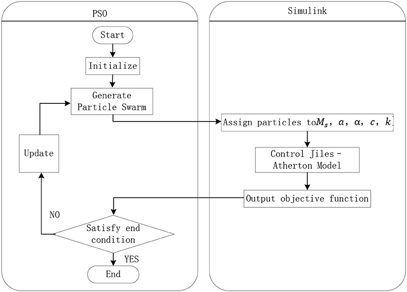
Figure 7. Flow diagram of parameters optimization of Jiles-Atherton model using PSO.

As shown in Figure 7, the PSO algorithm and J-A hysteresis model are connected by the five parameters of the model and the corresponding fitness of the particle. In the process of optimizing parameters of J-A model by PSO, PSO firstly generates particle swarm, and assigns the particles in the particle swarm to five parameters M_s, a, α, c, k of J-A model in turn. Then, utilizing the SIMULINK form of J-A model, the calculated values of the objective functions corresponding to these parameters are obtained. Finally, the calculated value is transferred to PSO as the fitness value of the particle to determine whether it can exit the algorithm.

During the simulation calculation of parameters of J-A model, the number of sampling points is set to 53. That means the number of sampling points equals to the number of measured magnetic flux density in this paper. The maximum value of current is set to 2A, which is the same condition with the experiment in this paper. For PSO simulation parameters, Swarm Size = 100. It indicates that there are 100 solution spaces. Maximum number of iterations MaxIter = 100. The minimum fitness is 0.00001. The search space of the five parameters are set to the area within±100% near their true values. Inertial factor w = 1. The acceleration constant c₁ = c₂ = 2.

Results and Discussions

Using the PSO parameter optimization method described above, the parameters of the hysteresis characteristic test results shown in Figure 5 are identified. The parameters of J-A hysteresis model for two damping channels of the MR fluid damper can be obtained, respectively, as shown in Table 1. In order to compare, this paper also uses the traditional optimization method of least squares method (LSM) to optimize the model parameters. The results are listed in Table 1 and compared with the optimization results of PSO method.

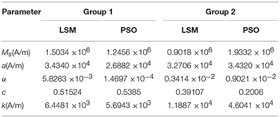
Table 1. Parameters optimization of J-A model for MR fluid damper.

The results of group 1 and group 2 are the calculation results of the data measured by sensor 1 and sensor 2, respectively. The results of parameter estimation by the two methods are shown in Table 1.

According to the optimized parameters in Table 1, the J-A hysteresis model curve can be plotted. The hysteresis curves of J-A hysteresis model under the PSO parameters and the LMS parameters are compared with experimental hysteresis curves as shown in Figure 8.

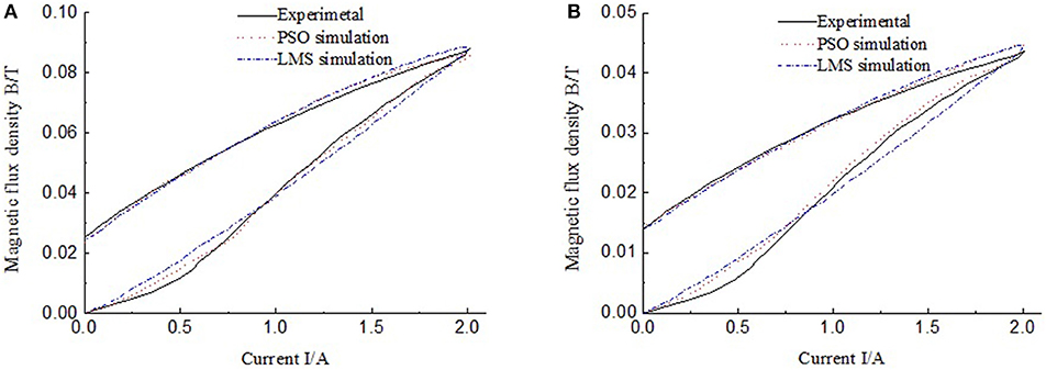
Figure 8. Comparison of hysteresis curve using different optimization methods. (A) Group 1; (B) Group 2.

Figures 8A,B show that, during the process of current increase, there are both small differences between the measured results and the curves drawn by J-A model under the LMS optimization method. In order to compare the accuracy of PSO and LSM methods, four kinds of errors are calculated from Figure 8 and listed in Table 2. Table 2 shows the max absolute errors, max relative errors, average errors and average relative errors of the two methods in prediction of ferromagnetic hysteresis curves of the MR damper. As we can see, the accuracy of PSO method is better than the LSM method on each position. The accuracy of the two methods is indicated by both the max relative error and the average relative error. Both the two relative errors show that the PSO method is better than the traditional LSM method in prediction of ferromagnetic hysteresis curves of the MR damper.

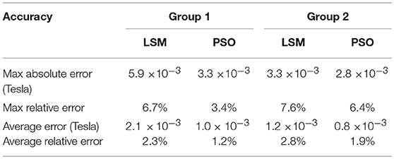
Table 2. Accuracy comparison of PSO and LSM methods on parameter identification of Jiles-Atherton model.

As we can see, for group 1, the relative errors of PSO are nearly half of those of LSM. For group 2, the relative errors of PSO are more than half of those of LSM. While, the variation of the magnetic flux density of group 1 is 0.09 Tesla and that of group 2 is 0.045 Tesla. The results in Table 2 indicate that the larger the variation range of magnetic flux density, the better the PSO method works.

Figure 9 shows the change of objective function with the number of iterations using LMS optimization method. And Figure 10 shows the change of objective function with the number of iterations using PSO optimization method.

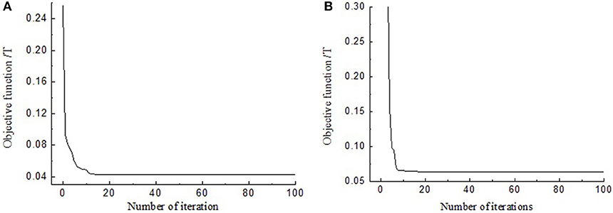
Figure 9. Changes of the value of the objective function with the numbers of iteration using LMS. (A) Group 1; (B) Group 2.

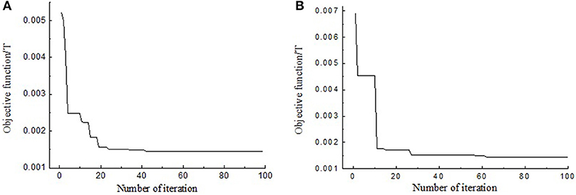
Figure 10. Changes of the value of the objective function with the numbers of iteration using PSO. (A) Group 1; (B) Group 2.

In order to compare the convergence speed of PSO and LSM methods, the results of magnetic induction stabilization at the same iteration numbers are listed in Table 3. The iteration times of 20 and 50 are both selected to reveal the variation trend of the convergence speed. Table 3 shows that when the iteration times reach to 20, the values of objective function using PSO are much smaller than that using LSM. Especially, for PSO, when the iteration times increases from 20 to 50, the values of objective function further decrease. However, for LSM, when the iteration times increases from 20 to 50, the values of objective function remain unchanged. The results indicate PSO has better global convergence ability than LSM on parameters optimization of hysteresis model of the MR damper.

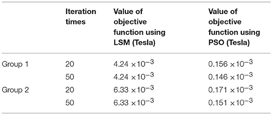
Table 3. Comparison of the value of objective function using LSM and PSO.

J-A model is described by a differential equation as shown in Equation (9). The equation contains the parameter δ which has relation to the direction of the magnetic flied. That means J-A model equation is discontinuous and non-differentiable at some point. For PSO, the optimized function is not required to be differentiable, derivative and continuous. While, LSM is an identification method based on process gradient information. Its premise is differentiable cost function, differentiable performance index and smooth search space.

In addition, there is some orders of magnitude difference for the five parameters of J-A model of the MR damper. This determines that the search space is unknown and stochastic. As PSO algorithm is based on the stochastic solution to optimize iteratively, it will leads to better optimization parameters than LSM.

Summary

In this paper, J-A hysteresis model is used to describe the hysteresis non-linearity of MR fluid dampers. According to the differential equation of J-A model, the numerical simulation model is established. The hysteresis characteristics test system of MR fluid damper is built. Then, the hysteresis loops of damping channels of the MR fluid damper in the working current range are obtained. The PSO optimization algorithm is applied to the parameter optimization of the model. Hence, five parameters of the model are optimized. The results of parameter optimization show that the hysteresis curves of MR fluid damper optimized by PSO algorithm is in good agreement with the experimental hysteresis loops compared with the traditional LMS optimization method. The hysteresis model and parameter identification of the MR fluid dampers in this paper provide support for eliminating or reducing the influence of hysteresis non-linearity on the performance of MR fluid dampers.

Author Contributions

ZL research the theory of the hysteresis model, built the experimental setup and wrote the manuscript. YG realized the simulation of the hysteresis model, parameter identification, and hysteresis characteristic test.

Funding

This work is supported by National Natural Science Foundation of China (NSFC) grant funded by the Chinese Government (No. 51305207) and Natural Science Foundation of Jiangsu Provincial College (Nos. 13KJB460010 and 17KJB413002).

Conflict of Interest Statement

The authors declare that the research was conducted in the absence of any commercial or financial relationships that could be construed as a potential conflict of interest.

References

Ahmadian, M., Appleton, R., and Norris, J. A. (2002). An analytical study of fire out of battery using magneto rheological dampers. Shock Vibrat. 9, 129–142. doi: 10.1155/2002/983140
Bingul, Z., and Karahan, O. (2011). “Tuning of fractional PID controllers using PSO algorithm for robot trajectory control,” in IEEE International Conference on Mechatronics, (Istanbul), 955–960.
Cao, S., Wang, B., Yan, R., Huang, W., and Yang, Q. (2004). Optimization of hysteresis parameters for the Jiles-Atherton model using a genetic algorithm. IEEE Trans. Appl. Superconduct. 14, 1157–1160. doi: 10.1109/TASC.2004.830462
Carlson, J. D. (2002). “What makes a good MR fluid?” in Electrorheological Fluids and Magnetorheological Suspensions. 63–69. doi: 10.1142/9789812777546_0010
Ge, P., and Jouaneh, M. (1997). Generalized preisach model for hysteresis nonlinearity of piezoceramicactuators. Precisi. Eng. 20, 99–111. doi: 10.1016/S0141-6359(97)00014-7
Gordaninejad, F., Wang, X., Hitchcock, G., Bangrakulur, K., Ruan, S., Siino, M., et al. (2010). Modular high-force seismic magneto-rheological fluid damper. J. Struct. Eng. 136, 135–143. doi: 10.1061/(ASCE)0733-9445(2010)136:2(135)
Hiemenz, G. J., Hu, W., and Wereley, N. M. (2009). Adaptive magnetorheological seat suspension for the expeditionary fighting vehicle. J. Phys. Con. Ser. 149:012054. doi: 10.1088/1742-6596/149/1/012054
Hsieh, Y. Z., Su, M. C., and Wang, P. C. (2014). A PSO-based rule extractor for medical diagnosis. J. Biomed. Inform. 49, 53–60. doi: 10.1016/j.jbi.2014.05.001
Jiles, D. C., and Atherton, D. L. (1986). Theory of ferromagnetic hysteresis. J. Magn. Magn. Mater. 61, 48–60. doi: 10.1016/0304-8853(86)90066-1
Jiles, D. C., and Atherton, D. L. (1998). Theory of ferromagnetic hysteresis. J. Appl. Phys. 55, 2115–2120. doi: 10.1063/1.333582
Jiles, D. C., Thoelke, J. B., and Devine, M. K. (1992). Numerical determination of hysteresis parameters for the modeling of magnetic properties using the theory of ferromagnetic hysteresis. IEEE Trans. Magn. 28, 27–35. doi: 10.1109/20.119813
Joseph, D. S. (2001). Parameter Identification for the Preisach Model of Hysteresis. Blacksburg, VA: VirginiaTech.
Kennedy, J. (2011). Particle swarm optimization/ /Encyclopedia of machine learning. Boston, MA: Springer, 760–766.
Leite, J. V., Avila, S. L., Batistela, N. J., Carpes, W. P., Sadowski, N., and Kuo-Peng, P., et al. (2004). Real coded genetic algorithm for Jiles-Atherton model parameters identification. Magn. IEEE Trans. 40, 888–891. doi: 10.1109/TMAG.2004.825319
Li, Z., Gong, Y., and Wang, J. (2019). Optimal control with fuzzy compensation for a magnetorheological fluid damper employed in a gun recoil system. J. Intell. Mater. Syst. Struct. 30, 677–688. doi: 10.1177/1045389X17754258
Marion, R., Scorretti, R., Siauve, N., Raulet, M. A., and Krahenbuhl, L. (2008). Identification of Jiles-Atherton Model Parameters Using Particle Swarm Optimization. IEEE Trans. Magn. 44, 894–897. doi: 10.1109/TMAG.2007.914867
Salvini, A., and Fulginei, F. R. (2002). Genetic algorithms and neural networks generalizing the Jiles-Atherton model of static hysteresis for dynamic loops. Magn. IEEE Trans. 38, 873–876. doi: 10.1109/20.996225
Seong, M. S., Choi, S. B., and Han, Y. M. (2009). Damping force control of a vehicle MR damper using a Preisach hysteretic compensator. Smart Mater. Struct. 18:074008. doi: 10.1088/0964-1726/18/7/074008
Shou, M., Liao, C., Zhang, H., Li, Z., and Xie, L. (2018). Modeling and testing of magnetorheological energy absorbers considering inertia effect with non-averaged acceleration under impact conditions. Smart Mater. Struct. 27:115028. doi: 10.1088/1361-665X/aae6a0
Singh, H. J., Hu, W., Wereley, N. M., Norman, M., and William, G., et al. (2014). Experimental validation of a magnetorheological energy absorber design optimized for shock and impact loads. Smart Mater. Struct. 23:125033. doi: 10.1088/0964-1726/23/12/125033
Trapanese, M. (2011). Identification of parameters of the Jiles-Atherton model by neural networks. J. Appl. Phys. 109:07D355. doi: 10.1063/1.3569735
Wilson, P. R., Ross, J. N., and Brown, A. D. (2001). Optimizing the Jiles-Atherton model of hysteresis by a genetic algorithm. IEEE Trans. Magn. 37, 989–993. doi: 10.1109/20.917182
Keywords: MR fluid damper, hysteresis, Jiles-Atherton model, parameter identification, nonlinear system
Citation: Li Z and Gong Y (2019) Research on Ferromagnetic Hysteresis of a Magnetorheological Fluid Damper. Front. Mater. 6:111. doi: 10.3389/fmats.2019.00111
Received: 18 December 2018; Accepted: 30 April 2019;
Published: 17 May 2019.
Edited by:
Marcelo J. Dapino, The Ohio State University, United StatesReviewed by:
Luwei Zhou, Fudan University, ChinaXufeng Dong, Dalian University of Technology (DUT), China
Copyright © 2019 Li and Gong. This is an open-access article distributed under the terms of the Creative Commons Attribution License (CC BY). The use, distribution or reproduction in other forums is permitted, provided the original author(s) and the copyright owner(s) are credited and that the original publication in this journal is cited, in accordance with accepted academic practice. No use, distribution or reproduction is permitted which does not comply with these terms.
*Correspondence: Zhaochun Li, lzc.hn@163.com