Vertical distribution of intraseasonal variation signals in the Kuroshio Current source area during 2018–2020

1 Introduction

The North Pacific Low Latitude Western Boundary Current (WBC) system plays an important role in the global climate and ocean material cycle due to its complex three-dimensional structure and strong multi-scale variabilities (Lukas et al., 1996; Hu et al., 2015). The Kuroshio Current (KC), generated by the bifurcation of the North Equatorial Current (NEC) east of the Philippine coast (Zhai et al., 2014), flows northeast along the Philippines and partly enters the South China Sea through the Luzon Strait (Chao, 1991; Qu, 2001; Wu and Chiang, 2007; Qu et al., 2009). The remainder flows into the eastern area of Taiwan Island, the East China Sea, and the southeastern region of Japan (Hu et al., 2015). Beneath this current, a southward subsurface flow called the Luzon Undercurrent (LUC) exists, which was discussed by Qu et al. (1997) through 14 repeated hydrological observations along 18°N. In recent years, the velocity structure and origin of the LUC have been extensively studied (Xie et al., 2009; Hu et al., 2013).

As important components of the WBC, the multi-scale temporal variations in both the KC and the LUC have been a focal point of extensive attention and research in recent years. Chen et al. (2020) used high-resolution mixed-coordinate ocean model reanalysis data from 1992 to 2016 to show that large-scale wind forcing in the tropical western Pacific plays a dominant role in the interdecadal variation in KC intrusion into the South China Sea. The results showed that the interannual variation in the KC was closely related to the bifurcation latitude of NEC and El Niño/Southern Oscillation (ENSO) (Qiu and Joyce, 1992; Qiu and Lukas, 1996; Zhai and Hu, 2013). At the seasonal time scales, Chen et al. (2015), using two sets of mooring data of the 18°N section, highlighted the seasonal dynamics of the KC, emphasizing its comparative strength during the spring and summer in the northern region and comparative weakness in autumn. Hu et al. (2013) argued that the LUC exhibits an increased intensity during the boreal winter while being comparatively weaker in spring.

At the intraseasonal time scales, Wang et al. (2014) used numerical simulation results to demonstrate that KC and LUC have significant intraseasonal variations at their origins. The change in the KC in the upper 500 m was discussed with onboard observations along 18°20’N in December 2006 and January 2008 but the measurement range did not cover the LUC completely (Kashino et al., 2009). Using direct measurements of three sets of Acoustic Doppler Current Profiles (ADCPs) deployed at 18°N east of Luzon Island between February 2018 and May 2020, Wang F. et al. (2022) found a significant intraseasonal signal with a period of 50–60 days in the upper KC source region. Hu et al. (2013) pointed out that the maximum southward velocity of LUC was around 650 m, and the LUC had a significant intraseasonal signal of 70–80 days based on direct measurements of ADCP at 18°N/122.7°E, which was closely related to the mesoscale eddies propagating westward. In this study, the significance of intraseasonal variations (ISVs) was assessed by calculating the percentage of the standard deviation of 20–90 day band-pass filtered sea surface height anomalies (SSHa) to the standard deviation of the daily SSHa (Figure 1). The percentage of ISVs in the KC region is between 40% and 60%, with an average of 50%. Therefore, it can be concluded that ISVs are of great significance to the KC region. In the coastal areas of Luzon Island, the percentage of ISVs is greater than 50%.

Figure 1 Annual mean ratio (color, percentage) for the standard deviation of 20–90 day band-pass filtered SSHa relative to the standard deviation of SSHa during 2018–2020, with three black circles indicating the location of three mooring stations.

Generally, the strong intraseasonal signals in the Philippine Sea are due to the influence of mesoscale eddies, intraseasonal long Rossby waves, nonlinear and Madden Julian Oscillation (Lin et al., 2005; Hu et al., 2013; Qiu et al., 2015; Hu et al., 2018). Investigations have shown that the impact of high-energy mesoscale eddies is very important for the KC east of the Philippines (Gilson and Roemmich, 2002; Chiang et al., 2015; Wang et al., 2016). Qiu et al. (2015) pointed out that the sub-thermocline western boundary circulation could divide into two components governed by distinct dynamical processes.

Previous studies have shown that the KC has a significant ISV of 20–120 days east of the Luzon Strait (Liang et al., 2008; Yang et al., 2012; Lien et al., 2014; Tsa et al., 2015; Wang and Oey, 2016; Andres et al., 2017; Wang et al., 2017). In contrast, few studies focused on the vertical distribution of ISVs in the KC source area because of a lack of in situ observations. Utilizing data obtained from three moorings strategically deployed at 18°N between January 2018 and May 2020, in conjunction with satellite altimeter data and outputs from the Ocean General Circulation Model (OGCM) for the Earth Simulator (OFES), this study investigates the characteristics and dynamic mechanisms of two types of ISVs observed in the KC source region.

2 Data

2.1 Acoustic doppler current profilers

To observe the western boundary current east of Luzon Island, we conducted a study with the support of the Northwest Pacific Ocean Circulation and Climate Experiment. Three moorings were strategically deployed at 122.7°E (M1), 123°E (M2), and 123.3°E (M3) along 18°N in January 2018 and successfully recovered in May 2020 (Figure 1). Each mooring was equipped with two 75kHz ADCPs positioned at a depth of around 450 m to measure the flow velocities. The ADCPs at moorings were configured to 60 bins/per hour and 8 m/per bin so that the two ADCPs could capture flow velocity in the upper 900 m. Notably, the downward-looking ADCP at M2 was broken, and the measurement depth was, therefore, limited to 450 m. To eliminate the tidal signal, the original measured data were averaged to daily data for the purposes of this paper. The mooring data are available at the Marine Science Data Center of the Chinese Academy of Sciences (http://dx.doi.org/10.12157/iocas.2021.0017).

2.2 Global sea surface height dataset

This study utilized a global sea surface height dataset from January 1993 to December 2021, with a spatial resolution of 0.25° × 0.25°. The ISVs in the KC source region were investigated using daily SSHa and correspondingly calculated sea surface geostrophic velocities, covering the period from January 2018 to May 2020. These products were obtained through the Archiving, Validation, and Interpretation of Satellite Oceanographic Products on the website https://marine.copernicus.eu/.

2.3 OFES output

Based on the MOM3 mode of Geophysical Fluid Dynamics Laboratory/National Oceanic and Atmospheric Administration, the OFES outputs cover an area of 75°S–75°N with a horizontal spatial resolution of 0.1° (Masumoto et al., 2004). This data set is divided into 54 layers with a variable resolution with depths from 2.5 to 5900 m. The data can be downloaded at the Asia-Pacific Data Research Center (http://apdrc.soest.hawaii.edu/data/data.php) at the University of Hawaii.

2.4 Eddy detection and tracking algorithm

In the last few decades, several studies have revealed distinct characteristics in eddy velocity fields (Olson, 1991; Dickey et al., 2008). These features include minimum velocities in the proximity of the eddy center and tangential velocities that increase approximately linearly with distance from the center before reaching a maximum value and then decaying.

Utilizing satellite and OFES data, we applied the automatic eddy detection algorithm for the high-resolution numerical product to detect eddies (Nencioli et al., 2010). The algorithm primarily uses some of the features of the mesoscale eddy velocity field and has four constraints: (a) in the east-west direction, the meridional velocity (u) changes symbol after passing through the center of the eddy and increases away from the center of the eddy; (b) in the north-south direction, the latitude velocity (v) changes symbol after passing through the center of the eddy, increases as it moves away from the center of the eddy, and aligns with the rotation of u; (c) there is a local minimum of the flow rate in the center of the eddy; (d) the direction of the velocity vector changes with continuous rotation in the center of the eddy, and the orientation of the two adjacent velocity vectors must be within the same or two adjacent quadrants of the eddy center. To effectively prevent eddy trajectory splitting, the search area selected in this study was 75 km.

3 Results

3.1 Mean meridional velocity structure

The time series of meridian velocities measured by ADCP at 122.7°E, 123°E, and 123.3°E along 18°N are shown in Figure 2. The KC is mainly distributed in the upper layer of 400 m, and its instantaneous velocity maximum on the sea surface can reach 2.5 m s^-1 at 122.7°E and gradually decrease to 0.8 m s^-1 at 123.3°E. There are clear seasonal variations at three stations in 2019, all being comparatively stronger in winter, spring and summer and weaker in autumn. In comparison, the mooring data at three stations do not show evidence of significant seasonal cycles in 2018. In the upper 200 m, the amplitude of the KC increases westward with most velocities exceeding 0.50 m s^-1 during the observation. There is a non-permanent southward LUC below the KC. At 122.7°E, the LUC only existed in May and June 2018, with a maximum velocity of 0.47 m s^-1; however, in 2019, LUC became stronger and persisted over a longer period.

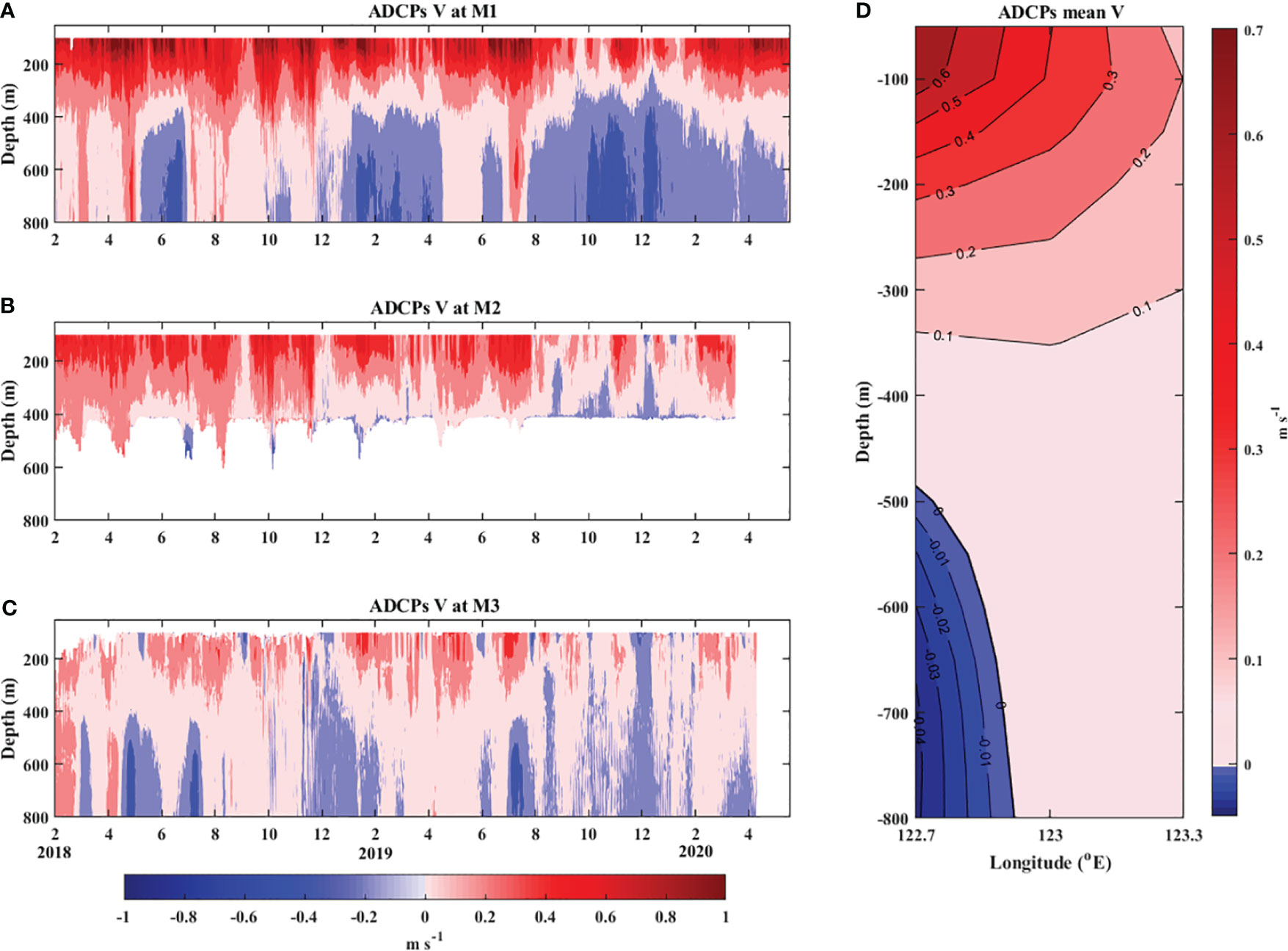
Figure 2 From January 2018 to May 2020, the meridional velocities observed at 18°N, (A) 122.7°E (M1), (B) 123°E (M2), and (C) 123.3°E (M3); (D) the time average of meridional velocities along 18°N based on three stations. Northward flow is set as positive (unit: m s^-1).

Using the observations of three moorings, the averaged meridional velocity distribution along 18°N was obtained by interpolation (Figure 2D). We found that the KC is mainly positioned above 400 m, its core is located west of 122.7°E, and the maximum northbound velocity is greater than 0.6 m s^-1. The intensity of the KC decreases with increasing longitude and depth. The LUC is mainly located west of 123°E, with a core depth of about 750 m and a maximum southward velocity of about 0.04 m s^-1.

3.2 Intraseasonal variability of KC and LUC

The LUC and KC exhibit significant intraseasonal variability (Ma et al., 2022). To better understand ISVs, we performed power spectral density (PSD) analysis on the meridional flow of three moorings at depths of 0–800 m. As shown in Figure 3, there are significant intraseasonal signals of 50–60 days and 80–100 days in the upper layers at three stations, and the intensity of the 50–60 days in the surface layer (0–200 m) gradually weakens from west to east, indicating that the signal is the strongest in the west. In the subsurface layer (500–800 m), there is a significant intraseasonal signal of 70–90 days at the M1 station but only 50–70 days intraseasonal signal at the M3 station.

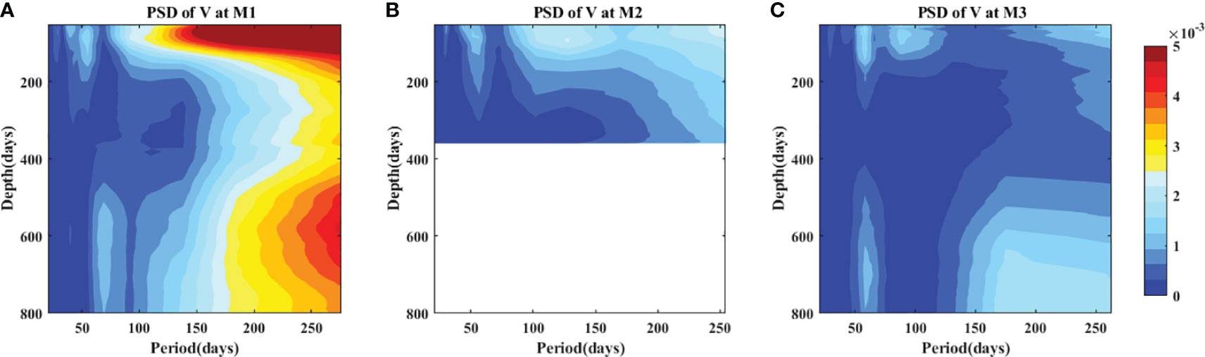
Figure 3 Power spectral density of the meridional velocities at (A) M1, (B) M2, and (C) M3 with depths during observation. Units are m²/(s² cycles per day [cpd]).

According to the observations, the peak PSD at M1 lacks coherence throughout the water column; hence, it is appropriate to calculate the power spectrum of the meridional flow in the surface and subsurface layers (Figures 4A, B, respectively). The surface intraseasonal spectral peak has a predominant peak of 56 days above 200 m, while the subsurface intraseasonal spectral peak is 73 days, which is consistent with the result shown in Figure 3. In comparison, the spectral peak in the surface layer at the M3 site is 56 days, while the peak in the subsurface layer is 60 days (Figures 4C, D).

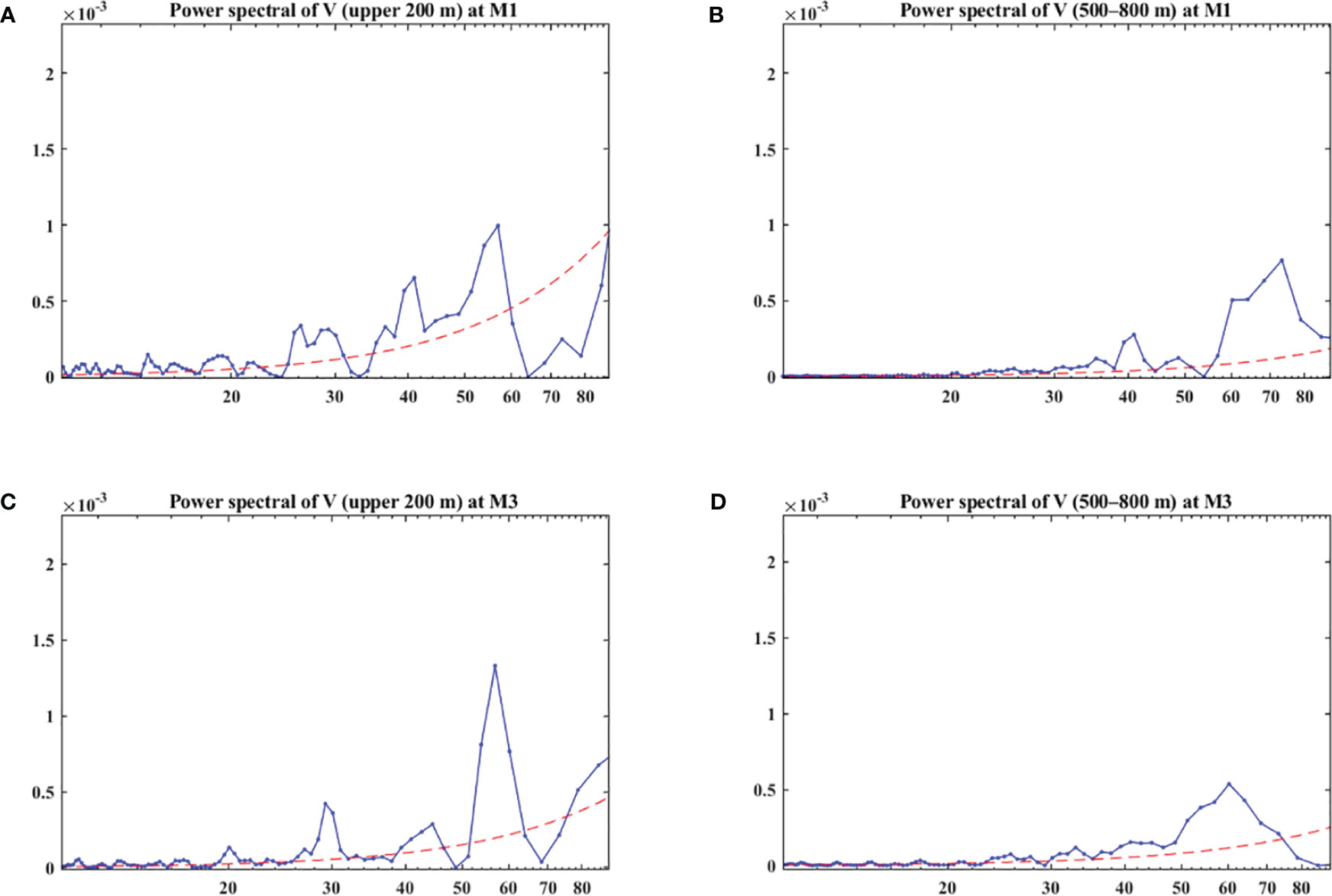
Figure 4 Power spectral of the meridional velocities in surface layer (0–200 m) and subsurface layer (500–800 m) obtained from ADCP measurements on M1 stations for (A, B) and on M3 stations for (C, D). The red dashed line indicates the 95% significance level. Units are m²/(s² cycles per day [cpd]).

To distinguish the two different periods of ISVs, the time series of the meridional flow at the M1 site under 10–60 day band-pass and 60–120 day band-pass filter are shown in Figure 5. The depiction highlights the vertical distribution of ISV signals characterized by two different frequencies. Higher-frequency ISV signals primarily exist in the surface layer above 200 m, and lower-frequency ISV signals typically appear below 400 m. In addition, the same filter was performed on M3 in Figures 5C, D. The intensity of high-frequency ISV in the surface layer was significantly lower than that at M1, confirming the westward enhancement of the surface ISV. Similarly, the intensity of low-frequency subsurface ISV on M3 was significantly weaker than on M1.

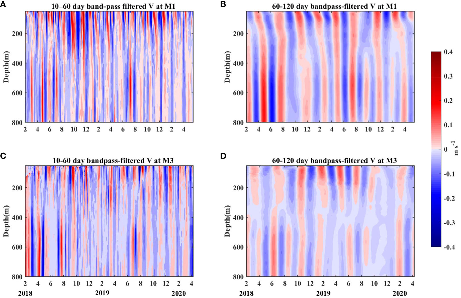
Figure 5 (A) 10-60 day band-pass filtered meridional velocities at M1. (B) 60-120 day band-pass filtered meridional velocities at M1. (C, D) are the same as (A, B), but at M3. Units are m s^-1.

The percentage of two types of ISVs in the total velocity variance at each depth derived from the mooring ADCP measurements is presented in Figure 6. The blue/red line is calculated by dividing the standard deviation of the meridional velocities under 10–60 d/60–120 d by that of the original meridional flows. At the M1 station, the contribution of high-frequency ISV above 150 m is greater than 50%. Its peak occurs at 150 m and gradually falls to about 30% with the increase in depth (Figure 6A). The contribution of low-frequency ISVs is small in the upper layer of 200 m and tends to decrease with the increase in depth. Below 200 m, it increases with depth to more than 40%, exceeding the contribution of high-frequency ISVs. The two types of ISVs exhibit distinct vertical structures and frequencies at the M1 site. As shown in Figures 6B, C, corresponding calculations showed that the increase/decrease structure of the subsurface ISV signals was more pronounced in 2018 than in 2019. Conversely, at the M3 station, the high-frequency ISV consistently assumes a dominant role (Figures 6D-F).

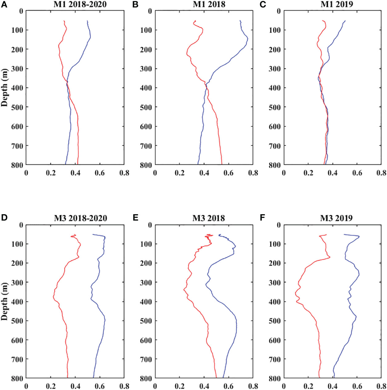
Figure 6 Percentage of two types of ISV signals in the total velocity variance at each depth derived from the mooring ADCP measurements. Blue and red lines indicate the meridional velocities under 10–60 d and 60–120 d band-passed filters, respectively. (A–C) represent the total time series, 2018, and 2019 on M1, respectively; (D–F) indicate those on M3.

3.3 Vertical distribution of EKE east of the Luzon strait

In this analysis, ADCP data at M1 and M3 stations are employed to investigate the spatial distribution of ISVs along 18°N. Figure 7 presents the calculated time series of eddy kinetic energy (EKE) at both stations, utilizing the following formula:

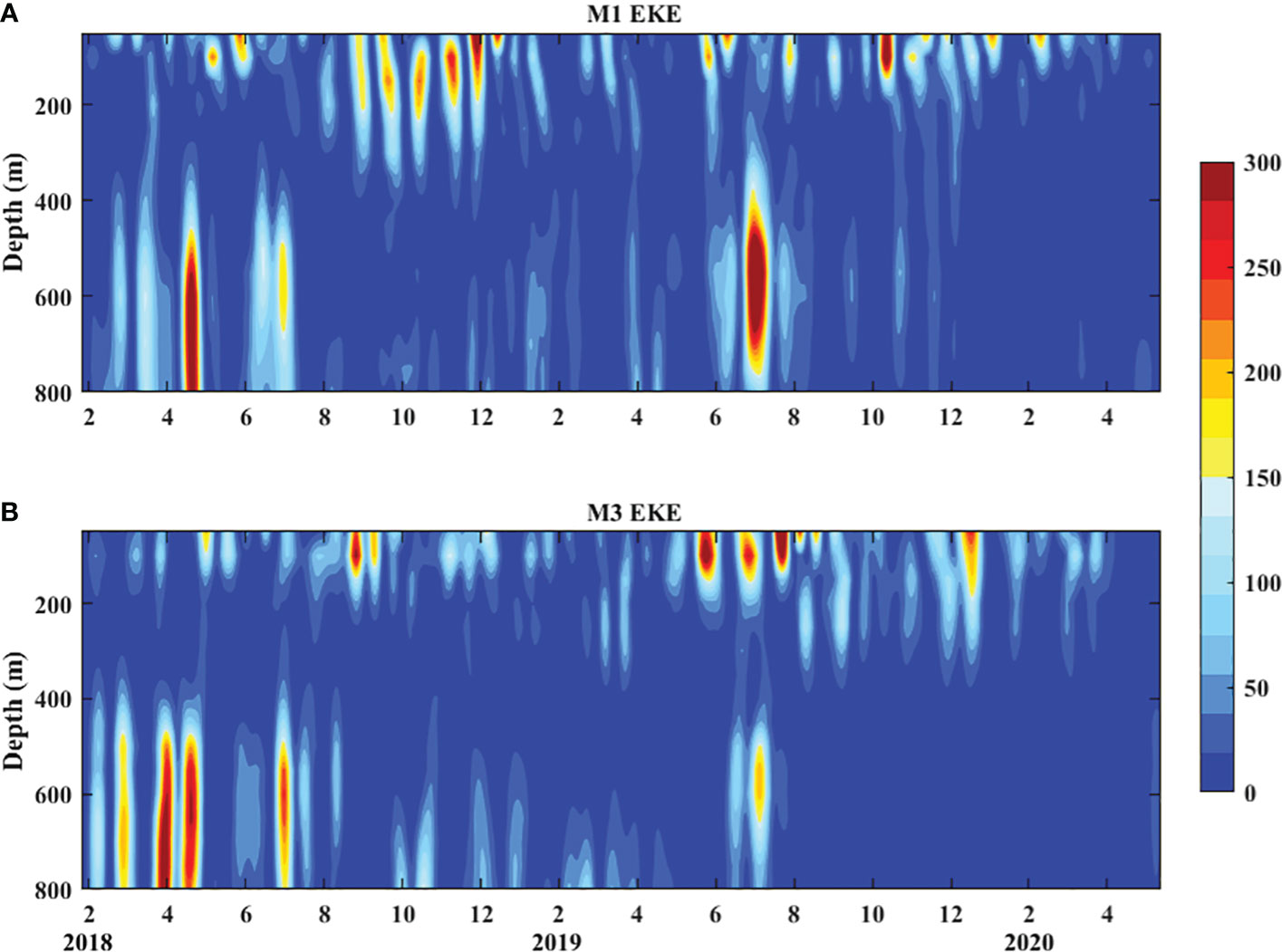
Figure 7 Time series of EKE (unit: cm² s^-2) calculated from mooring observations on (A) M1 and (B) M3 between January 2018 and May 2020.

where ${\text{u}}^{\prime }$and ${\text{v}}^{\prime }$ represent zonal and meridional velocity anomalies filtered by the 20–90 day Lanczos band-pass filter. Generally, the EKE on M1 and M3 was stronger in 2018 than in 2019. In the surface layer, the EKE at the M1 station was stronger than that at the M3 station, suggesting a prevailing westward strengthening trend. However, in the subsurface layer, the EKE at M3 was stronger than that at M1 in 2018. Furthermore, the ISV signals were not obvious at either station in 2019, with only a singular peak occurring in July.

Generally, the OFES output is consistent with observations and has been widely used in numerous studies (Zhang et al., 2014; Xu et al., 2019; Zhang et al., 2021). Wang Z. et al. (2022) compared velocity anomalies from OFES output at 800 m at 13°N/130°E from October 2014 to October 2015 with ADCP measurements, both of which showed significant ISVs. Zhang et al. (2021) demonstrated a strong agreement between the OFES output transports at 8°N/127°E during the period from December 2010 to August 2014, aligning well with mooring measurements. The study also presented a reliable reproduction of the seasonal signal of subsurface EKE.

To explore why the intraseasonal signals in 2018 were stronger than in 2019, the annual averaged EKE in the surface layer and subsurface layer in 2018 and 2019 is depicted in Figure 8. In the surface layer, the EKE north of Luzon Island and east of Taiwan Island was much higher in 2018 than in 2019. In the subsurface layer, the high EKE around the mooring stations in 2018 occurred predominantly in the 18°N–20°N region, while the high EKE region in 2019 was predominantly north of 20°N. Around three mooring stations, stronger eddy activity in 2018 led to a more pronounced enhanced ISVs compared with that in 2019 (Figures 6).

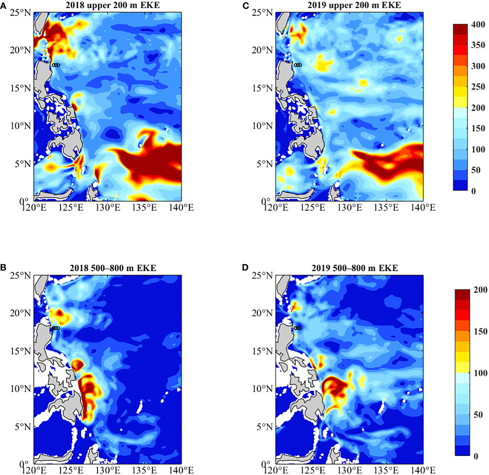
Figure 8 Averaged EKE (unit: cm² s^-2) in the (A) surface layer and (B) subsurface layers in 2018 and (C) surface layer and (D) subsurface layers in 2019 based on OFES outputs. The black circles denote three moorings.

Using the OFES output, Figures 9 illustrates the annual mean distributions of vertical EKE from 2001 to 2019. Along the coast of Luzon Island (122°E–124°E), the eddy activity was concentrated in the surface layer at 200 m and gradually intensified northward, as illustrated in Figure 9A. Along the 18°N zonal axis, as depicted in Figure 9B, the eddy activity in the surface layer is notably intensified along the coastal region, which is consistent with the result from Figure 7. At the latitude of 18°N where the mooring is located, there is a clear EKE peak below 400 m both in Figures 9A, B. Consequently, the vertical distribution of the two types of ISVs is mainly caused by locally generated surface and subsurface eddies.

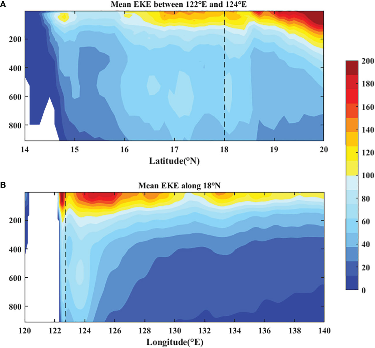
Figure 9 During the period 2001–2019, the averaged EKE (unit: cm² s^-2) based on the OFES output: (A) between 122°E and 124°E, (B) long 18°N. The black dotted line represents the M1 station.

3.4 Eddy detection

Although ADCP measurements capture the vertical structure and ISV of KC/LUC, these single-point observations are still insufficient to describe the spatial structure of KC/LUC. The time series of geostrophic velocity obtained by satellite altimetry is consistent with the mean value of the 150 m upper layer measured by ADCP (Wang F. et al., 2022). This observation indicates that the satellite altimeter data effectively captures the sea surface ISV signal, as observed by the mooring. Consequently, the satellite altimetry products prove convenient to investigate the ISVs in the KC source region.

Figure 10A shows a time-longitude diagram of the SSHa along the latitude 18°N. The ISV signals of SSHa clearly propagate towards the west. Its phase velocity was calculated as -0.11 m s^-1, which was consistent with the phase velocity of the first baroclinic Rossby wave at 18°N (Chelton and Schlax, 1996). Furthermore, the intensification of westward-propagating eddies in the KC region is apparent west of 140°E, aligning closely with the westward-enhanced ISV signals. The ISV of the KC may be related to baroclinic Rossby waves and eddies.

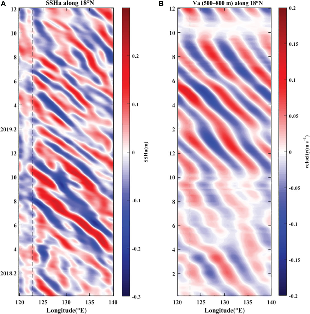
Figure 10 (A) Based on satellite data, 10–60 day band-pass filtered SSHa (unit: m) along 18°N during 2018–2019; (B) the meridional velocity anomalies (unit: m s^-1) under 60–120 day band-pass filter in 500–800 m along 18°N during 2018–2019 from OFES output. The black dotted line represents the M1 station.

Figure 10B shows the time-longitude diagram of the subsurface meridional velocity anomaly under 60–120 day band-pass filter east of the KC source area along 18°N. Similarly, the ISV signals gradually increase as they move westward. In July 2019, the reversal of the LUC (Ma et al., 2022) resulted in a strong positive meridional velocity anomaly in the subsurface layer. This occurrence was consistent with the enhancement of subsurface EKE on the M1 station in July 2019.

Satellite altimeter data and OFES output data from 2018 and 2019 were employed to detect surface and subsurface eddy trajectories over a two-year period. Assuming that the initial position of each eddy trajectory represents its generation position, the results of the eddy tracking are shown in Figure 11. The number of eddies is counted in each 2° × 2° box. At the sea surface, a large number of eddies are generated between the western boundary and 145°E, as depicted in Figures 11A, C. The majority of these eddies propagate westward, with a velocity close to the first baroclinic Rossby (Qiu and Chen, 2010), a phenomenon regulating the ISV of the surface current (Figure 10A). Notably, more eddies were generated near the mooring area in 2018 than in 2019. These eddies strengthened west of 140°E, resulting in stronger intraseasonal signals in the surface layer along the western boundary in 2018. In the subsurface layer, a smaller number of eddies were generated during the two-year period, with 163 and 126 subsurface eddies in 2018 and 2019, respectively, the majority occurring in close proximity to the western boundary and around 140°E. Most of the subsurface eddies also tended to move westward, affecting the ISV of subsurface currents (Figure 10B).

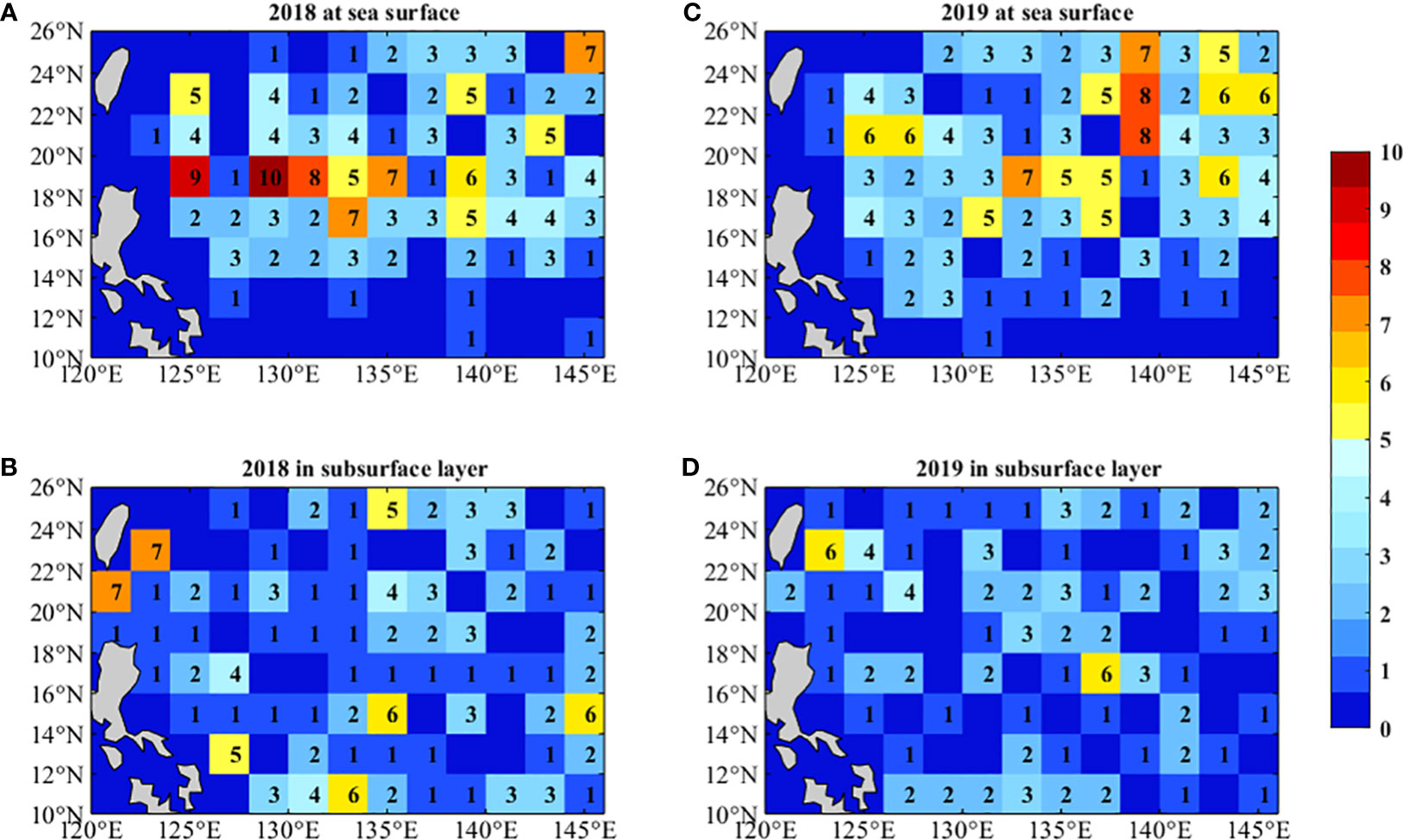
Figure 11 Spatial distribution of the eddy numbers generated in the 2° × 2° box (A) at sea surface in 2018 with satellite data, (B) in subsurface layer in 2018 from OFES data, (C) at sea surface in 2019 with satellite data, and (D) in subsurface layer in 2019 from OFES data.

3.5 Energy analysis

Ocean eddies derive their energy from both horizontal and vertical shear instability in the ocean interior (Qiu and Chen, 2004; Qiu et al., 2009; Qiu et al., 2015). To evaluate the contribution of barotropic and baroclinic instability in regulating surface and subsurface ISVs, we calculated the barotropic conversion rate (BT) and baroclinic conversion rate (BC) in surface and subsurface layers from 2001 to 2019 based on the OFES output.

where ${\text{u}}^{\prime }$ and ${\text{v}}^{\prime }$ are zonal and meridional velocity anomalies under the 20–90-day band-pass filter; $\tilde{\text{u}}$ and $\tilde{\text{v}}$ under 90 day of low-pass filter were used as the background ocean states; ${\text{ρ}}^{\prime }$ and ${\text{ω}}^{\prime }$ are potential density and vertical velocity under 20–90 day band-pass filter; $\text{g}$ and ${\text{ρ}}_0$ represent the gravitational constant and background potential density, respectively.

Time-averaged BT and BC in the surface layer are depicted in Figures 12A, B. A notable concentration of strong positive BT was observed north of Luzon Island, while the negative values were observed off the coast of the Philippines, which transitioned to positive values in the southeastern Philippine Sea. The BC is distinctly positive near the Luzon Strait south of Taiwan Island and off the northern coast of the Philippines, before turning negative south of 8°N. In the surface layer of three mooring stations, the calculated positive BC surpasses the absolute BT, indicating a significant energy shift from the eddy available potential energy to the eddy kinetic energy in this region. The enhanced eddy activities mean that more eddies move through the KC source area in a constant period, that increases the likelihood of strengthened surface high-frequency ISVs. In Figures 12C, D, the BC in the subsurface layer is consistently positive north of 10°N, while BT has a large negative value along the western boundary. To compare the vertical structure of BT and BC quantitatively, the longitude-depth of BT and BC along 18°N is averaged from 2001 to 2019, based on OFES output calculated in Figure 13. In the subsurface layer, a pronounced negative BT prevails west of 122.8°E, while the positive BC is notably smaller than the absolute value of BT. Consequently, at the M1 station, the dominant influence is attributed to the BT. As the negative BT converts the eddy kinetic energy into mean kinetic energy, the LUC characterized by a low frequency of ISV with a period of 70–80 days exists on M1. On the M3 station in the subsurface layer, the BT turns from negative to positive, and the positive BC is smaller than the positive BT. This results in LUC not having sufficient kinetic energy, which is consistent with the observed absence of LUC at 123.3°E/18°N. Consequently, there is no discernable subsurface low-frequency ISV enhancement at the M3 site.

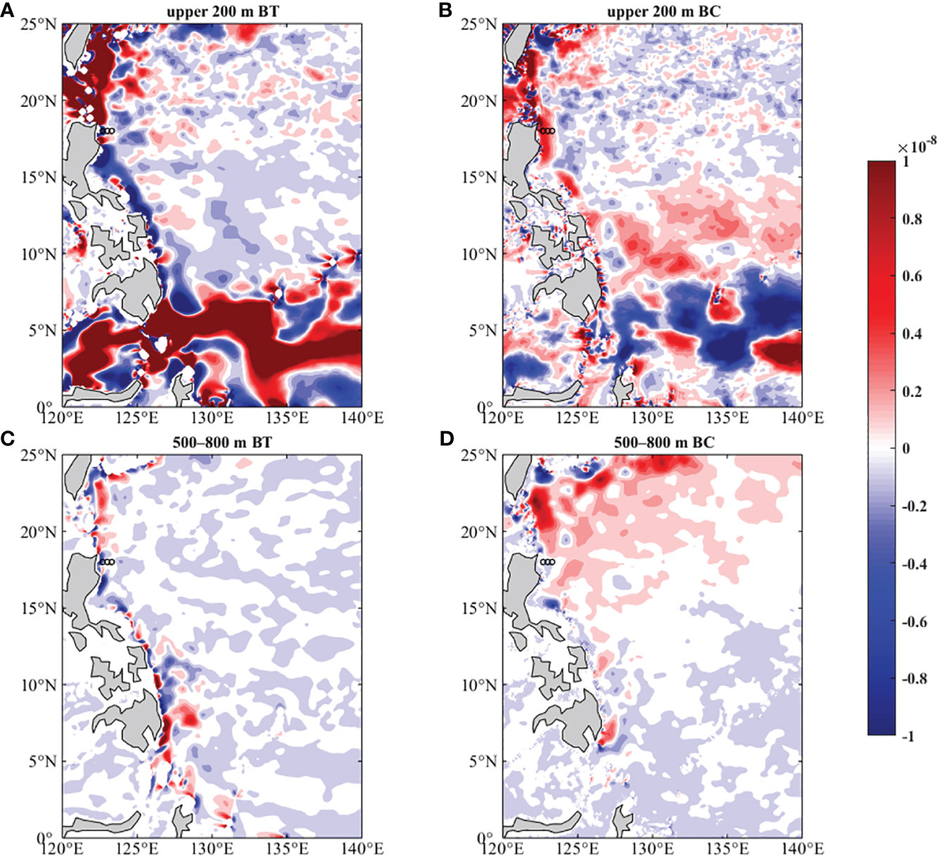
Figure 12 Averaged (A) barotropic conversion rate and (B) baroclinic conversion rate in the surface layer (0–200 m) from 2001 to 2019, followed by based on OFES outputs; (C) and (D) are the same as (A) and (B), but in the subsurface layer (500–800 m). The black circles denote three moorings. Units are m² s^-3.

Figure 13 Vertical (A) barotropic conversion rate and (B) baroclinic conversion rate along 18°N averaged from 2001 to 2019 based on OFES output. The black dotted lines represent the M1 and M3 stations. Units are m² s^-3.

4 Discussion and conclusions

Utilizing ADCP measurements at longitudinal positions 122.7°E, 123°E, and 123.3°E along the 18°N latitude in the KC source region from 2018 to 2020, an investigation of the vertical distribution of ISVs was carried out. During the observation period, the averaged KC was primarily situated above 400 m with a maximum flow of about 0.6 m s^-1, and its core was located west of 122.7°E. The LUC below the KC is located west of 123°E and below 500 m with a core at 750 m. PSD analysis indicated that the meridional surface KC had a 56-day ISV signal, exhibiting a westward propagation and strengthening trend. In comparison, the subsurface at 122.7°E/18°N exhibited a more prolonged period of enhanced ISV signals (73 days), while the subsurface at 123.3°E/18°N recorded a shorter duration of 60 days of ISV signals.

As westward propagating mesoscale eddies are an important source of the oceanic ISV in the Philippine Sea (Hu et al., 2018), the eddy trajectories that can affect surface and subsurface eddies at 18°N, 122.7°E are depicted in Figure 14. Most eddies that can affect the mooring position (within 150 km from mooring stations) are locally generated between the western boundary and 130°E. These eddies propagate westward and then dissipate before reaching the western boundary, which plays an important role in the ISV of the KC. As the EKE distribution and eddy tracking analysis indicates that 2018 is an eddy-rich year, the seasonal variability of the KC was not distinct, and the strengthening/weakening trend of the two types of ISVs along the coast was more pronounced in 2018.

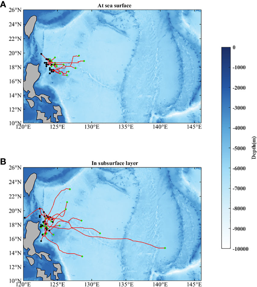
Figure 14 (A) Trajectories of eddies (red curve) calculated from satellite data in 2018–2019 that can arrive at 18°N, 122.7°E, (B) Same as (A), but for subsurface eddy obtained from the OFES outputs during the same period. The green dots denote the starts of those eddies, and the black dots denote their destinations.

The interaction of mean currents and eddies has a non-negligible impact on ISV (Hu et al., 2013; Wang F. et al., 2022). Yan et al. (2019) pointed out that both barotropic and baroclinic instabilities contribute to the generation of eddy kinetic energy in the KC region north of 20°N. In the KC source region, the baroclinic conversion plays a dominant role in the surface layer, signifying an energy shift from the mean current to eddies and the presence of strengthened surface high-frequency ISVs. Combined with the spatial distribution of the eddy numbers and the eddy trajectories in the same period, eddies in the subsurface layer are relatively fewer in number and predominantly situated at western boundary. The strong negative BT at 122.7°E/18°N converts the energy from the eddy into the mean flow. This phenomenon increases the likelihood of the appearance of LUC at the M1 station. At the M3 station, the BT turns from negative to positive and the positive BC is smaller than the positive BT, suggesting the LUC not having sufficient kinetic energy. As the LUC is characterized by a low frequency of ISV, the two types ISV signals are more distinct at the M1 station than at the M3 station.

Data availability statement

The original contributions presented in the study are included in the article/supplementary material. Further inquiries can be directed to the corresponding author.

Author contributions

HG: Software, Writing – original draft. FW: Investigation, Writing – original draft. FL: Methodology, Writing – review & editing. LZ: Data curation, Writing – review & editing. DH: Formal analysis, Writing – review & editing.

Funding

The author(s) declare financial support was received for the research, authorship, and/or publication of this article. This research was financially supported by Laoshan Laboratory (LSKJ202201601), the Strategic Priority Research Program of the Chinese Academy of Sciences (grant XDB42010105), and the National Key Research and Development Program of China (2020YFA0608801). Mooring data were collected onboard R/V KeXue implementing the open research cruise NORC2022-09 supported by the NSFC Shiptime Sharing Project (Grant No. 42249909) and the Project of Science and Technology Innovation of Laoshan Laboratory (Grant No. LSKJ202201702).

Acknowledgments

We express our sincere gratitude to all scientists and technicians on R/V Science and Science 3 for the deployment and retrieval of the subsurface moorings used in this work.

Conflict of interest

The authors declare that the research was conducted in the absence of any commercial or financial relationships that could be construed as a potential conflict of interest.

Publisher’s note

All claims expressed in this article are solely those of the authors and do not necessarily represent those of their affiliated organizations, or those of the publisher, the editors and the reviewers. Any product that may be evaluated in this article, or claim that may be made by its manufacturer, is not guaranteed or endorsed by the publisher.

References

Andres M., Mensah V., Jan S., Chang Y.-J., Lee C. M., Ma B., et al. (2017). Downstream evolution of the Kuroshio’s time-varying transport and velocity structure. J. Geophys. Res. 122 (5), 3519–3542. doi: 10.1002/2016JC012519
Chao S. Y. (1991). Circulation of the East China Sea, a numerical study. J. Oceanogr. 46, 273–295. doi: 10.1007/BF02123503
Chelton D. B., Schlax M. G. (1996). Global observations of oceanic Rossby waves. Science 272 (5259), 234–238. doi: 10.1126/science.272.5259.234
Chen Z., Wu L., Qiu B., Li L., Hu D., Liu C., et al. (2015). Strengthening Kuroshio observed at its origin during November 2010 to October 2012. J. Geophys. Res. 120 (4), 2460–2470. doi: 10.1002/2014JC010590
Chen Y., Zhai F., Li P. (2020). Decadal variation of the Kuroshio Intrusion Into the South China Sea during 1992–2016. J. Geophys. Res. 125 (1), e2019JC015699. doi: 10.1029/2019JC015699
Chiang T.-L., Wu C.-R., Qu T., Hsin Y.-C. (2015). Activities of 50–80 day subthermocline eddies near the Philippine coast. J. Geophys. Res. 120, 3606–3623. doi: 10.1002/2013JC009626
Dickey T. D., Nencioli F., Kuwahara V. S., Leonard C., Black W., Rii Y. M., et al. (2008). Physical and bio-optical observations of oceanic cyclones west of the island of Hawai’i. Deep-Sea Res. II 55 (10-13), 1195–1217. doi: 10.1016/J.DSR2.2008.01.006
Gilson J., Roemmich D. (2002). Mean and temporal variability in Kuroshio geostrophic transport south of Taiwan, (1993–2001). J. Oceanogr. 58 (1), 183–195. doi: 10.1023/A:1015841120927
Hu D., Hu S., Wu L., Li L., Zhang L., Diao X., et al. (2013). Direct measurements of the Luzon undercurrent. J. Phys. Oceanogr. 43 (7), 1417–1425. doi: 10.1175/JPO-D-12-0165.1
Hu S., Sprintall J., Guan C., Sun B., Wang F., Yang G., et al. (2018). Spatiotemporal features of intraseasonal oceanic variability in the Philippine Sea from mooring observations and numerical simulations. J. Geophys. Res. 123 (7), 4874–4887. doi: 10.1029/2017JC013653
Hu D., Wu L., Cai W., Sen Gupta A., Ganachaud A., Qiu B., et al. (2015). Pacific western boundary currents and their roles in climate. Nature 522, 299–308. doi: 10.1038/nature14504
Kashino Y., Espana N., Syamsudin F., Richards K. J., Jensen T., Dutrieux P., et al. (2009). Observations of the hoorth equatorial current, mindanao current, and kuroshio current system during the 2006/07 el Niño and 2007/08 la Niña. J. Oceanogr. 65 (3), 325–333. doi: 10.1007/s10872-009-0030-z
Liang W., Yang Y., Tang T., Chuang W.-S. (2008). Kuroshio in the Luzon strait. J. Geophys. Res. 113 (C8), C08048. doi: 10.1029/2007JC004609
Lien R. C., Ma B., Cheng Y. H., Ho C. R., Qiu B., Lee C. M., et al. (2014). Modulation of kuroshio transport by mesoscale eddies at the Luzon strait entrance. J. Geophys. Res. 119 (4), 2129–2142. doi: 10.1002/2013JC009548
Lin X., Wu D., Li Q., Lan J. (2005). An amplification mechanism of intraseasonal long Rossby wave in subtropical ocean. J. Oceanogr. 61 (2), 369–378. doi: 10.1007/s10872-005-0047-x
Lukas R., Yamagata T., McCreary J. P. (1996). Pacific low-latitude western boundary currents and the Indonesian throughflow. J. Geophys. Res. 101 (C5), 12209–12216. doi: 10.1029/96JC01204
Ma J., Hu S., Hu D., Villanoy C., Wang Q., Lu X., et al. (2022). Structure and variability of the Kuroshio and Luzon undercurrent observed by a mooring array. J. Geophys. Res. 127 (2), e2021JC017754. doi: 10.1029/2021JC017754
Masumoto Y., Sasaki H., Kagimoto T., Komori N., Ishida A., Sasai Y., et al. (2004). A fifty-year eddy-resolving simulation of the world ocean-Preliminary outcomes of OFES (OGCM for the Earth Simulator). J. Earth Simul. 1, 35–56. doi: 10.32131/jes.1.35
Nencioli F., Dong C., Dickey T., Washburn L., Mcwilliams J. C. (2010). A vector geometry-based eddy detection algorithm and its application to a high-resolution numerical model product and high-frequency radar surface velocities in the Southern California Bight. J. Atmos. Ocean. Technol. 27, 564–579. doi: 10.1175/2009JTECHO725.1
Olson D. B. (1991). Rings in the ocean. Annu. Rev. Earth Planet. Sci. 19, 283–311. doi: 10.1146/annurev.ea.19.050191.001435
Qiu B., Chen S. (2004). Seasonal modulations in the eddy field of the South Pacific Ocean. J. Phys. Oceanogr. 34, 1515–1527. doi: 10.1175/1520-0485(2004)034<1515:SMITEF>2.0.CO;2
Qiu B., Chen S. (2010). Interannual variability of the North Pacific subtropical countercurrent and its associated mesoscale eddy field. J. Phys. Oceanogr. 40 (1), 213–225. doi: 10.1175/2009JPO4285.1
Qiu B., Chen S., Kessler W. S. (2009). Source of the 70-day mesoscale Eddy variability in the coral sea and the North Fiji Basin. J. Phys. Oceanogr. 39, 404–420. doi: 10.1175/2008JPO3988.1
Qiu B., Chen S., Rudnick D. L., Kashino Y. (2015). A new paradigm for the North Pacific subthermocline low-latitude western boundary current system. J. Phys. Oceanogr. 45 (9), 2407–2423. doi: 10.1175/JPO-D-15-0035.1
Qiu B., Joyce T. M. (1992). Interannual variability in the mid- and low latitude western north pacific. J. Phys. Oceanogr. 22, 1062–1079. doi: 10.1175/15200485(1992)022<1062:IVITMA>2.0.CO;2
Qiu B., Lukas R. (1996). Seasonal and interannual variability of the north Equatorial Current, the Mindanao Current, and the Kuroshio along the Pacific western boundary. J. Geophys. Res. 101 (C5), 12315–12330. doi: 10.1029/95JC03204
Qu T. D. (2001). Role of ocean dynamics in determining the mean seasonal cycle of the South China Sea surface temperature. J. Geophys. Res. 106 (C4), 6943–6955. doi: 10.1029/2000JC00479
Qu T., Kagimoto T., Yamagata T. (1997). A subsurface countercurrent along the east coast of Luzon. Deep Sea Res: Part I. 44 (3), 413–423. doi: 10.1016/S0967-0637(96)00121-5
Qu T., Song Y., Yamagata T. (2009). An introduction to the South China Sea throughflow: Its dynamics, variability, and application for climate. Dynam. Atmos. Oceans. 47, 3–14. doi: 10.1016/j.dynatmoce.2008.05.001
Tsa C., Andres M., Jan S., Mensah V., Sanford T. B., Lien R.-C., et al. (2015). Eddy-Kuroshio interaction processes revealed by mooring observations off Taiwan and Luzon. Geophys. Res. 42 (19), 8098–8105. doi: 10.1002/2015GL065814
Wang F., Li Y., Wang J. (2016). Intraseasonal variability of the surface zonal currents in the western tropical Pacific Ocean: characteristics and mechanisms. J. Phys. Oceanogr. 46, 3639–3660. doi: 10.1175/JPO-D-16-0033.1
Wang J., Oey L. Y. (2016). Seasonal exchanges of the kuroshio and shelf waters and their impacts on the shelf currents of the east China Sea. J. Geophys. Res. 46 (5), 1615–1632. doi: 10.1175/JPO-D-15-0183.1
Wang Q., Tang Y. M., Pierini S., Mu M. (2017). Effects of singular-vector-type initial errors on the short-range prediction of Kuroshio extension transition processes. J. Climate. 30 (15), 5961–5983. doi: 10.1175/JCLI-D-16-0305.1
Wang Q., Zhai F., Hu D. (2014). Variations of Luzon undercurrent from observations and numerical model simulations. J. Geophys. Res. 119 (6), 3792–3805. doi: 10.1002/2013JC009694
Wang F., Zhang L., Feng J., Hu D. (2022). Atypical seasonal variability of the kuroshio current affected by intraseasonal signals at its origin based on direct mooring observations. Sci. Rep. 12, 13126. doi: 10.1038/s41598-022-17469-5
Wang Z., Zhang L., Hui Y., Wang F., Hu D. (2022). Two flavors of intraseasonal variability and their dynamics in the north equatorial current/undercurrent region. Front. Mar. Sci. 9. doi: 10.3389/fmars.2022.845575
Wu C. R., Chiang T. L. (2007). Mesoscale eddies in the northern South China Sea. Deep-Sea Res. II. 54, 1575–1588. doi: 10.1016/j.dsr2.2007.05.008
Xie L., Tian J., Hu D., Wang F. (2009). A quasi-synoptic interpretation of water mass distribution and circulation in the western North Pacific II: Circulation. J. Oceanol. Limnol. 27 (4), 955–965. doi: 10.1007/s00343-009-9161-8
Xu A., Yu F., Nan F. (2019). Study of subsurface eddy properties in northwestern Pacific Ocean based on an eddy-resolving OGCM. Ocean. Dyn. 69, 463–474. doi: 10.1007/s10236-019-01255-5
Yan X., Kang D., Curchitser E. T., Pang C. (2019). Energetics of eddy-mean flow interactions along the western boundary currents in the North Pacific. J. Phys. Oceanogr. 49, 789–810. doi: 10.1175/JPO-D-18-0201.1
Yang D., Yin B., Liu Z., Bai T., Qi J., Chen H. (2012). Numerical study on the pattern and origins of Kuroshio branches in the bottom water of southern East China Sea in summer. J. Geophys. Res. 117 (C2), C02014. doi: 10.1029/2011JC007528
Zhai F., Hu D. (2013). Revisit the interannual variability of the north equatorial current transport with ECMWF ORA-S3. J. Geophys. Res. 118 (3), 1349–1366. doi: 10.1002/jgrc.20093
Zhai F., Wang Q., Wang F., Hu D. (2014). Decadal variations of Pacific North Equatorial Current bifurcation from multiple ocean products. J. Geophys. Res. 119, 1237–1256. doi: 10.1002/2013JC009692
Zhang L., Hu D., Hu S., Wang F., Wang F., Yuan D. (2014). Mindanao Current/Undercurrent measured by a subsurface mooring. J. Geophys. Res. 119 (6), 3617–3628. doi: 10.1002/2013JC009693
Keywords: intraseasonal variation, Kuroshio current, eddy, barotropic conversion, baroclinic conversion
Citation: Gong H, Wang F, Liu F, Zhang L and Hu D (2024) Vertical distribution of intraseasonal variation signals in the Kuroshio Current source area during 2018–2020. Front. Mar. Sci. 11:1303565. doi: 10.3389/fmars.2024.1303565
Received: 28 September 2023; Accepted: 04 January 2024;
Published: 22 January 2024.
Edited by:
Chunyan Li, Louisiana State University, United StatesReviewed by:
Fangguo Zhai, Ocean University of China, ChinaHailong Liu, Chinese Academy of Sciences (CAS), China
Copyright © 2024 Gong, Wang, Liu, Zhang and Hu. This is an open-access article distributed under the terms of the Creative Commons Attribution License (CC BY). The use, distribution or reproduction in other forums is permitted, provided the original author(s) and the copyright owner(s) are credited and that the original publication in this journal is cited, in accordance with accepted academic practice. No use, distribution or reproduction is permitted which does not comply with these terms.
*Correspondence: Fujun Wang, fujunwang@qdio.ac.cn