A nitrogen isoscape of phytoplankton in the western North Pacific created with a marine nitrogen isotope model

1 Introduction

Identifying the migration routes of marine animals is crucial for sustainable fisheries management and biodiversity conservation. Many methods, such as catch per unit effort with location (e.g., Thorson et al., 2016), dart tag/capture studies (e.g., Hanselman et al., 2015), and bio-logging (e.g., Hays et al., 2016), are used to study the migration routes. Although tracking technologies have advanced greatly, the migration routes over the entire life cycle of marine animals, including the spawning sites or the larval and juvenile habitats, are often unknown due to body size limitations (Lowerre-Barbieri et al., 2019). Chemical signatures in otoliths and other body parts have become a promising tool for tracing these migration routes (Tzadik et al., 2017).

The isotopic composition of animal tissues and local environments can be used as a natural tag to track an animal’s movements through isotopically distinct habitats, called iso-logging (Matsubayashi et al., 2022). Nitrogen isotope (δ¹⁵N) analysis of incremental growth tissues, such as eye lenses and vertebral bones, has proven promising for reconstructing migration routes and feeding environments over the animal’s life (Matsubayashi et al., 2017; Matsubayashi et al., 2020; Vecchio and Peebles, 2020; Harada et al., 2022). It is essential to understand the spatial variations in δ¹⁵N values (nitrogen isoscapes) across the habitat for using the δ¹⁵N values for iso-logging of marine animals. However, seamless nitrogen isoscapes are generally difficult to obtain through field sampling (McMahon et al., 2013; Matsubayashi et al., 2020; Fripiat et al., 2021) because there are wide spatial and temporal variations in δ¹⁵N values.

The variations in δ¹⁵N values reflect biogeochemical processes. When phytoplankton assimilates nitrate, nitrogen isotopes are fractionated (Wada and Hattori, 1978; Montoya and McCarthy, 1995). The δ¹⁵N value of nitrate (δ¹⁵N_Nitrate) increases as nitrate consumption increases due to an isotopic effect ranging from 5‰ to 8‰ during nitrate assimilation by phytoplankton (Granger et al., 2010). When denitrification occurs in the water column, the δ¹⁵N_Nitrate value increases dramatically due to a strong isotopic effect of ~15‰ (Granger et al., 2008). N₂-fixation produces fixed nitrogen with a δ¹⁵N value of ~0‰, because nitrogen fixers take up N₂ with little isotopic effect (Minagawa and Wada, 1986). This fixed nitrogen with a low δ¹⁵N value is eventually converted into nitrate with a low δ¹⁵N value through the degradation of nitrogenous organic compounds via remineralization and subsequent nitrification. The spatial patterns of δ¹⁵N_Nitrate values in the euphotic zone are conserved in phytoplankton and are subsequently transferred to organisms with higher trophic positions (zooplankton and fish) with ¹⁵N enrichment of ~3‰ per trophic position (Minagawa and Wada, 1984).

In this study, we developed a marine nitrogen isotope model that includes biogeochemical processes, and we generated a seamless nitrogen isoscape of phytoplankton as the base of the food web (δ¹⁵N_Base) in the western North Pacific for iso-logging studies. The western North Pacific, the focus of this article, is one of the most biologically diverse and productive fishery regions (FAO, 2022). Identifying fish movements in the western North Pacific is commercially important for pelagic fish in countries in the Asia–Pacific region.

2 Model description

2.1 Nitrogen isotope model

The marine nitrogen isotope model used in this study has seven compartments: phytoplankton (PHY), diazotrophs (DIA), zooplankton (ZOO), particulate organic nitrogen (PON), dissolved organic nitrogen (DON), nitrate (NO₃⁻), ammonium (NH₄⁺), and dinitrogen (N₂) (Figure 1). The prognostic variables are the N and ¹⁵N concentrations of these compartments, except N₂. The concentration of N₂ is set to always be sufficient for DIA and the δ¹⁵N value is set as 0‰. The equations for the N and ¹⁵N cycles are essentially the same as those used by previous modeling studies in the western North Pacific (Yoshikawa et al., 2005; Yoshikawa et al., 2016; Yoshikawa et al., 2022). The parameters and isotopic fractionation factors used here are shown in Tables 1, 2, respectively. The N₂ fixation and denitrification schemes are introduced in this study.

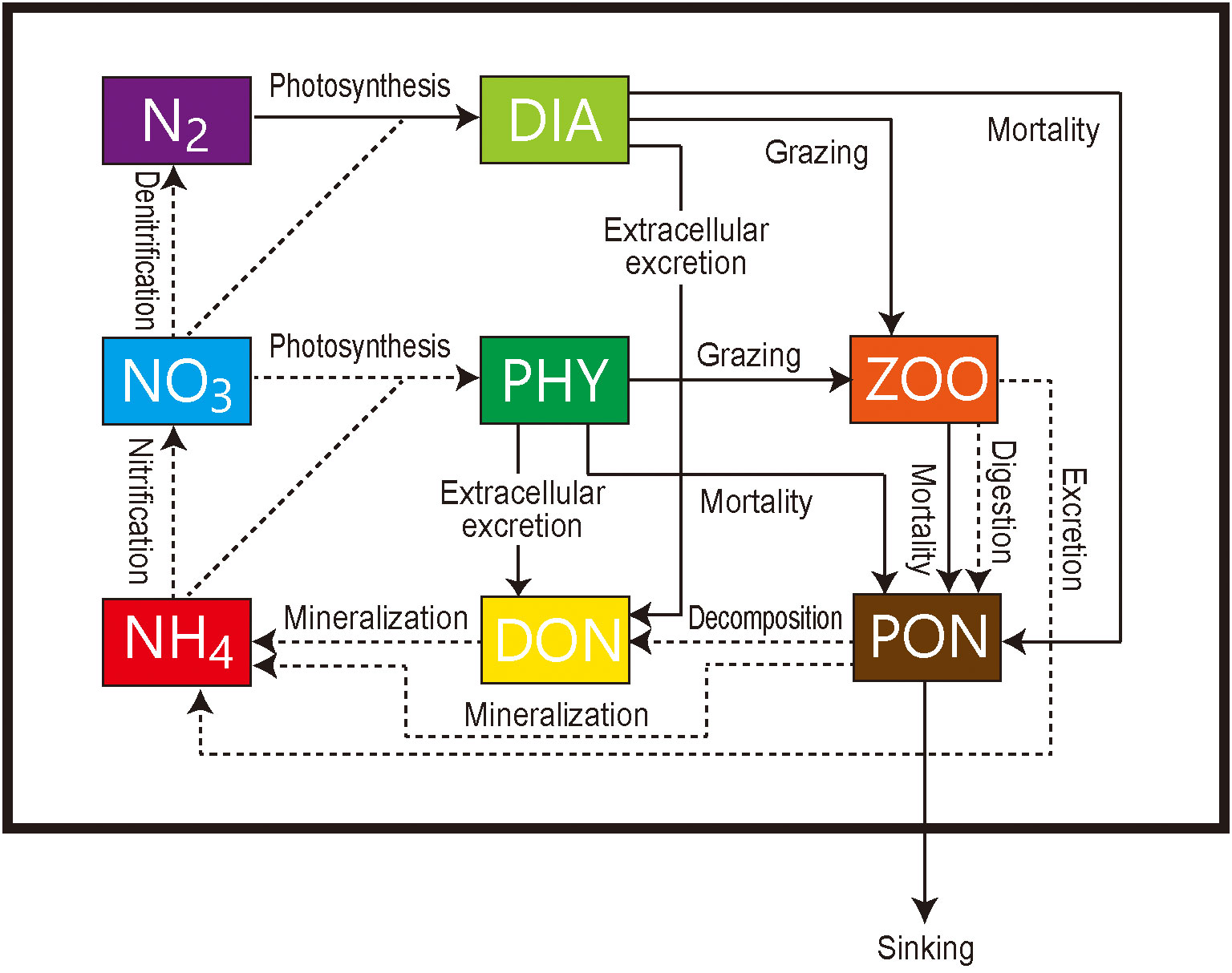
Figure 1 Schematic of the marine ecosystem isotope model. NO₃⁻, nitrate concentration; NH₄⁺, ammonium; N₂, dinitrogen; PHY, phytoplankton; DIA, diazotrophs; ZOO, zooplankton; PON, particulate organic nitrogen; DON, dissolved organic nitrogen. Dashed and solid arrows indicate nitrogen flows with and without isotopic fractionation, respectively.

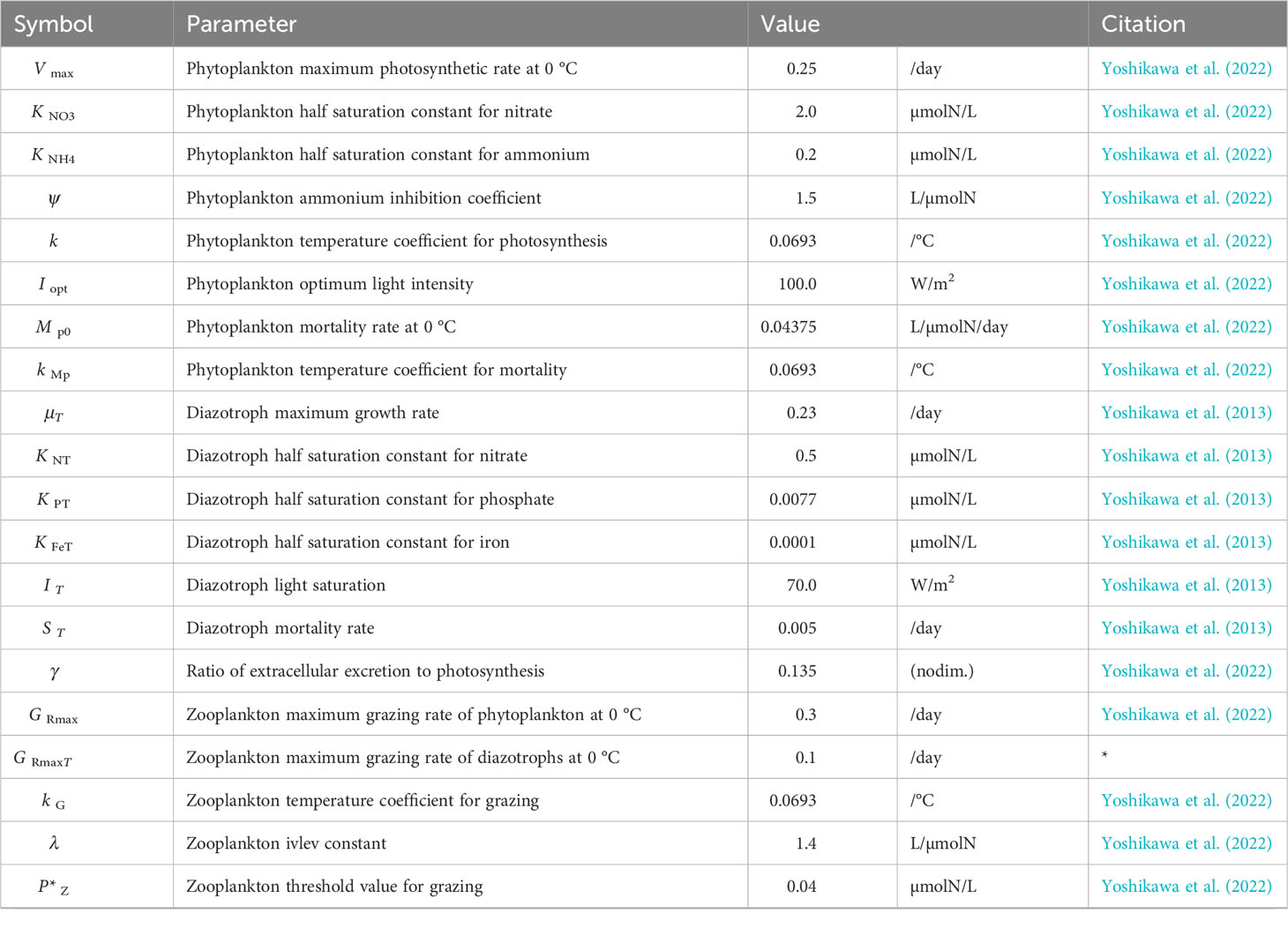
Table 1 Biological parameters in the nitrogen isotope model.

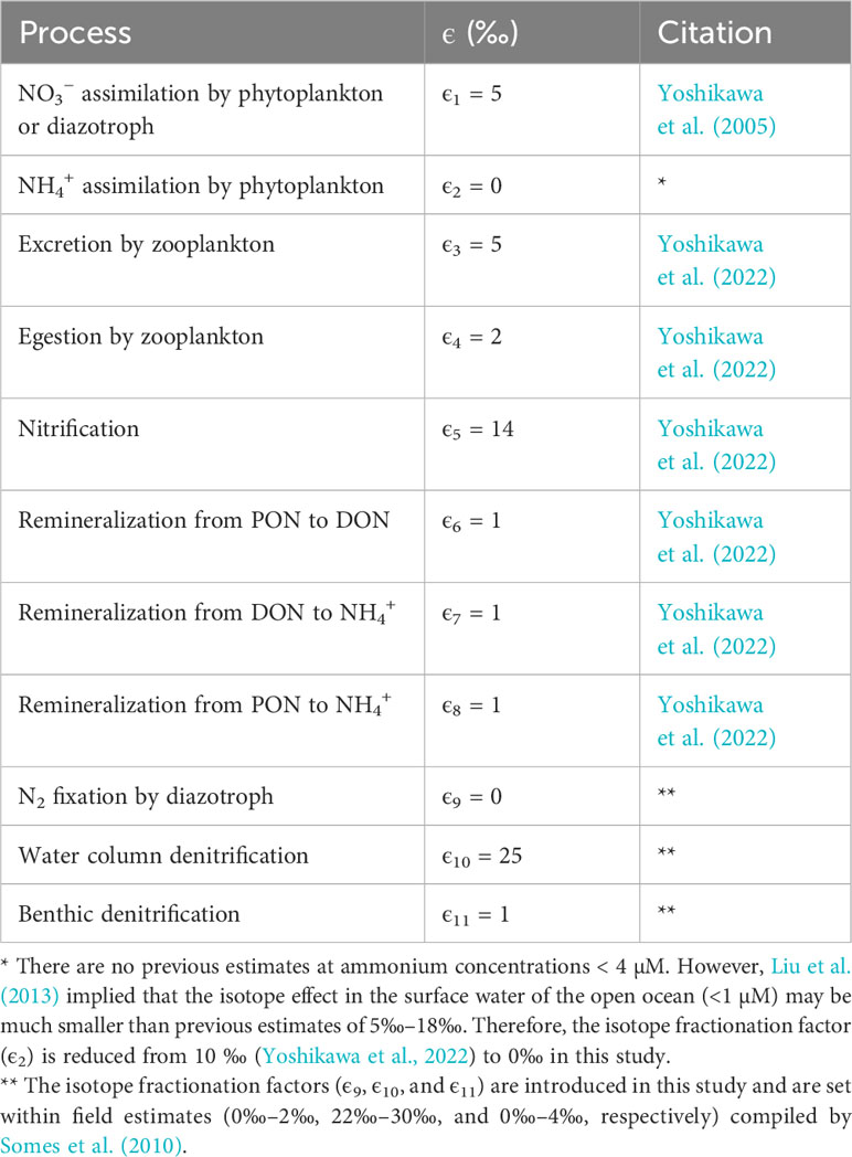
Table 2 Isotope fractionation factors in the nitrogen isotope model.

2.2 N₂ fixation and denitrification

The N₂ fixation scheme is a modified version of the model developed by Hood et al. (2001) (see also Coles et al., 2004; Hood et al., 2004; Coles and Hood, 2007; Yoshikawa et al., 2013). The prognostic variable of DIA is calculated as a function of time, t, and each grid using the following governing equations.

Growth _DIA in Equation 1 is modeled by:

which describes light-, dissolved inorganic phosphorous (DIP)-, and Fe-dependent variations in diazotroph growth. In Equation 2, μ_T is the maximum growth rate. Variable I is the irradiance, and I_T is the light saturation parameter. In addition, K_PT and K_FeT are half-saturation constants for diazotroph DIP and Fe uptake. Diazotrophs fix N₂ with 0‰ and no isotopic fractionation (ϵ₉). The diazotroph nitrate uptake is modeled by:

where K_NT is the half-saturation constant for nitrate. Although diazotrophs take up nitrate, their growth rate is not limited by nitrate availability. Thus, when nitrate concentrations are very low, diazotroph growth is supported almost entirely by N₂ fixation.

Mortality _DIA in Equation 1 is modeled using:

where S_T is the mortality rate of DIA.

Grazing _DIA in Equation 1 is modeled using:

where G_RmaxT, λ, and P*z are the zooplankton maximum grazing rate for DIA, zooplankton Ivlev constant, and zooplankton threshold value for grazing, respectively. Variable T is the temperature, and K_G is the zooplankton temperature coefficient for mortality.

Extracellular Excretion _DIA in Equation 1 is modeled by:

where γ is the ratio of extracellular excretion of DIA to growth.

The water-column denitrification scheme is essentially the same as that reported by Schmittner et al. (2008). Oxygen consumption in suboxic waters (<3 µM) is inhibited and replaced by the oxygen-equivalent oxidation of nitrate:

Denitrification consumes nitrate at a rate of 80% of the oxygen equivalent rate, according to:

where R_O:N is the ratio of O to N. D_flag limits the rate of water column N-loss at a given nitrate threshold of D_min:

The isotopic fractionation factor for water-column denitrification (ϵ₁₀) is set to 25‰.

The benthic denitrification scheme is essentially the same as that reported by Shigemitsu et al. (2016). The benthic denitrification flux is parameterized based on the organic carbon flux to the seafloor (F_{POC_bot}) and bottom water O₂ and NO₃^– concentrations ([O₂]_bottom and [NO₃^–]_bottom) as:

where α_BD is tuned to set the globally integrated rates of benthic denitrification in the model to the rates within the range of previous estimates (80–140 Tg N yr^–1; Bianchi et al., 2012; Bohlen et al., 2012; DeVries et al., 2013; Somes et al., 2013; Shigemitsu et al., 2016; Somes et al., 2017). The isotopic fractionation factor for benthic denitrification (ϵ₁₁) is set to 1‰.

2.3 Offline biogeochemical model

The nitrogen isotope model was incorporated into the ocean general circulation model (COCO) with an offline method (Oka et al., 2008; Shigemitsu et al., 2016). The model has 256 × 198 grid points in the horizontal direction and 44 vertical layers. The horizontal resolution is about 1°, and the vertical spacing varies from 5 m at the top to 250 m at the bottom. The concentration of biogeochemical tracers is calculated by the following tracer equation:

where C is the tracer concentration, v is the velocity, K_H and K_V are the horizontal and vertical diffusivity, and S_C is the source/sink term for the tracer due to biogeochemical processes. The model was driven by climatological monthly mean physical fields (horizontal ocean velocities, vertical diffusivity, temperature, salinity, sea surface height, sea surface wind speed, sea ice fraction, and sea surface solar radiation) obtained from the outputs of a pre-industrial control simulation performed with an Earth system model (MIROC-ESM) (Watanabe et al., 2011) as in Shigemitsu et al. (2017). The climatological monthly mean concentration of dissolved iron was obtained from the output of a pre-industrial control simulation performed with an ocean biogeochemical model including an iron cycle (Yamamoto et al., 2019). In order to rapidly reach steady state, the initial conditions were set to values that have already reached steady state and were within the range of observations. The initial conditions of the nitrogen, phosphate, and oxygen concentrations were obtained from the outputs of a pre-industrial control simulation with MIROC-ESM (Watanabe et al., 2011). The initial conditions of δ¹⁵N of PHY, DIA, ZOO, PON, DON, NO₃⁻, and NH₄⁺ were set to constant values of 3‰, 0‰, 6‰, 6‰, 6‰, 5‰, and 6‰, respectively. The results of the simulations presented here are shown after 3000 years of time integration.

3 Results

3.1 Horizontal distributions of nitrate and chlorophyll a concentrations

The simulated distributions of annual mean nitrate and chlorophyll a concentrations in the surface layer are generally consistent with the climatological annual mean concentrations of the World Ocean Atlas 2018 (Garcia et al., 2019) and the SeaWiFS satellite data (O’Reilly et al., 1998), respectively (Figure 2). The model represents the high nitrate concentrations exceeding 5 µM observed in the subarctic region and the low concentrations below 2 µM observed in the subtropical region (Figures 2A, C). Because of the nitrate availability, the simulated chlorophyll a concentrations are also high in the subarctic region and low in the subtropical region (Figures 2B, D). The root-mean-square error (RMSE), which is an estimate of the absolute magnitude of the difference between the observed and modeled values, is relatively high in the northwestern North Pacific for both nitrate and chlorophyll a concentrations (Figures 2E, F). This is because of the lack of terrestrial inputs of nitrogenous nutrients in the model and its coarse resolution. The extremely high RMSE in the coastal region for the chlorophyll a concentration may also be attributed to the difficulty of satellite-based chlorophyll a estimation caused by terrestrial inputs of colored dissolved organic matter or suspended particles.

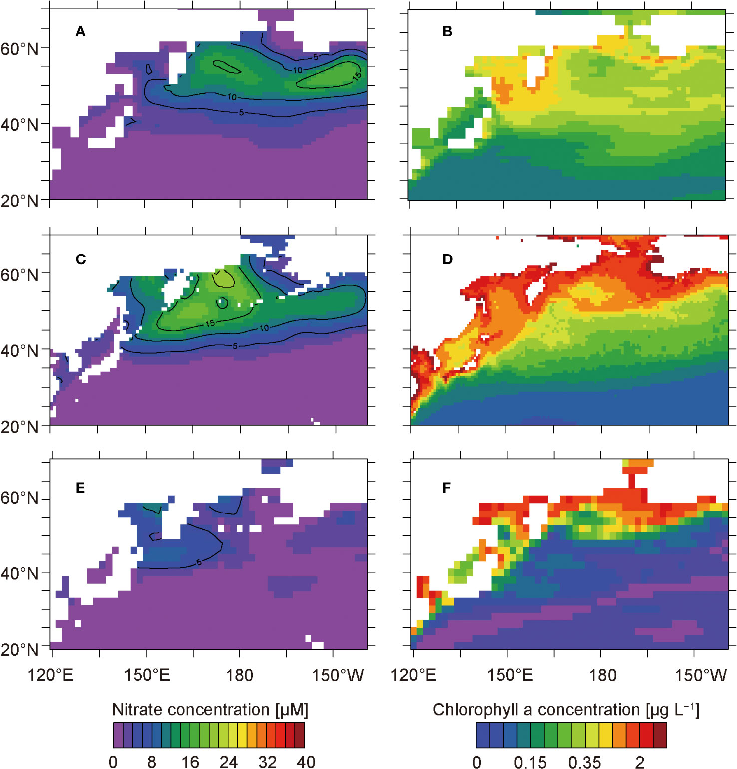
Figure 2 Concentrations of annual mean nitrate and chlorophyll a at the surface from the model simulations (A, B) and observations (C, D). Panels (C, D) show the climatological annual mean nitrate concentrations in the surface waters of the World Ocean Atlas 2018 (Garcia et al., 2019) and the climatological annual mean chlorophyll a concentrations based on the SeaWiFS satellite data from 1997 to 2006 (O’Reilly et al., 1998), respectively. Panels (E, F) show the root-mean-square error of the model simulations of nitrate and chlorophyll a concentrations, respectively.

3.2 Horizontal distributions of δ¹⁵N_Nitrate, δ¹⁵N_{Phytoplankton}, and δ¹⁵N_PON values

The simulated annual mean δ¹⁵N values of nitrate in the surface layer and phytoplankton and PON in the euphotic layers have similar high–low distributions, except in the Bering Strait (Figure 3). The model represents the ¹⁵N depletion observed in the subtropical and subarctic regions and the ¹⁵N enrichment observed in the Oyashio–Kuroshio transition region. The model also represents the overall observed ¹⁵N enrichment of nitrate and ¹⁵N depletion of phytoplankton.

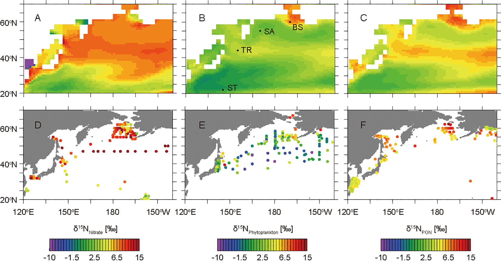
Figure 3 Horizontal δ¹⁵N distributions of annual mean nitrate, phytoplankton, and PON from the model simulations (A−C) and observations (D−F). Panels (A-C) show the δ¹⁵N_Nitrate values at the surface layer, the weighted average of δ¹⁵N_{Phytoplankton} values in the layers at 0−200 m, and the weighted average of δ¹⁵N_PON values in the layers at 0−200 m, respectively. Panels (D-F) show the shallowest δ¹⁵N_Nitrate values compiled by Rafter et al. (2019) and Fripiat et al. (2021), the δ¹⁵N_Base values estimated from the δ¹⁵N measurements of bulk nitrogen and amino acids of zooplankton (Matsubayashi et al., 2022), and the δ¹⁵N values of surface sediments compiled by NICOPP (Tesdal et al., 2013), respectively. Locations of the western subtropical North Pacific site (ST: 145°E, 22°N), the Kuroshio–Oyashio transition zone site (TR: 155°E, 44°N), the western subarctic North Pacific site (SA: 170°E, 55°N), and the Bering Strait region site (BS: 190°E, 60°N) selected for this study are shown.

The simulated values are not precisely consistent with the observed values shown in Figure 3 for the following reasons. The simulated δ¹⁵N_Nitrate values (Figure 3A) are annual mean surface values, whereas the observed values (Figure 3D) are the shallowest data that were measured in a single expedition compiled by Rafter et al. (2019) and Fripiat et al. (2021). The simulated δ¹⁵N_Phytplankton values (Figure 3B) are the weighted averages of the euphotic layer throughout the year, whereas the observed values (Figure 3E) are the δ¹⁵N_Base values estimated from the δ¹⁵N measurements of bulk nitrogen and amino acids of zooplankton obtained from various depths and seasons (Matsubayashi et al., 2022). The simulated δ¹⁵N_PON values (Figure 3C) are the weighted averages of the euphotic layer throughout the year, whereas the observed values (Figure 3F) are the δ¹⁵N_Bulk values of surface sediments obtained from various depths and redox conditions compiled by NICOPP (Tesdal et al., 2013), which could be affected by digenesis.

For the discussion, we selected four representative sites in the western subtropical North Pacific (ST: 145°E, 22°N), the Kuroshio–Oyashio transition zone (TR: 155°E, 44°N), the western subarctic North Pacific (SA: 170°E, 55°N), and the Bering Strait region (BS: 190°E, 60°N) (Figure 3). The simulated δ¹⁵N_Nitrate values in the surface layer are 1.1‰ at ST, 7.3‰ at TR, 6.8‰ at SA, and 6.6‰ at BS (Figure 3A). In the uppermost 200 m layers, the simulated weighted averages of δ¹⁵N_{Phytoplankton} are 0.6‰ at ST, 3.9‰ at TR, 2.1‰ at SA, and 6.7‰ at BS (Figure 3B), whereas those of δ¹⁵N_PON are 1.8‰ at ST, 5.9‰ at TR, 3.7‰ at SA, and 7.3‰ at BS (Figure 3C).

3.3 Seasonal cycles of nitrate, ammonium and phytoplankton concentrations

At ST, the simulated nitrate in the surface layer is depleted to<0.2 µM throughout the year and shows a slight increase from February to March (Figure 4A). The simulated ammonium accumulates slightly up to 0.02 µM in the layers at depths of 40–80 m from April to November (Figure 4B). The simulated phytoplankton concentration is low (<0.1 µM), equivalent to 0.2 μg Chl L^–1, throughout the year and has a small bloom in April (Figure 4C).

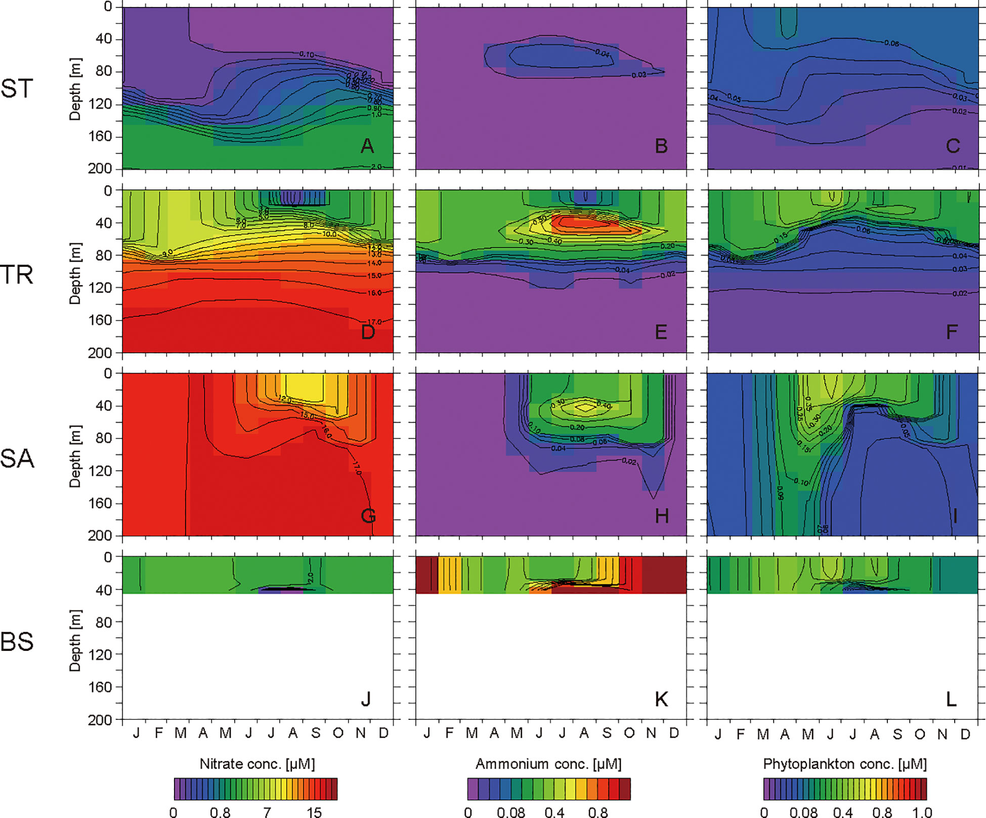
Figure 4 Seasonal cycles of simulated concentrations of nitrate, ammonium, and phytoplankton in the layers at 0−200 m at the western subtropical North Pacific site ST (A−C), the Kuroshio–Oyashio transition zone site TR (D−F), the western subarctic North Pacific site SA (G−I), and the Bering Strait region site BS (J−L).

At TR, the simulated nitrate in the surface layer reaches a maximum concentration of 8.5 µM in March and is depleted to 0.3 µM in August (Figure 4D). Then, until March, the nitrate concentration increases as the surface mixed layer deepens. The simulated ammonium accumulates to >0.3 µM in the layers at 30–60 m from May to November, and the maximum concentration is 0.9 µM at a depth of 40 m in August (Figure 4E). The simulated phytoplankton has high concentrations of >0.1 µM throughout the year and has a bloom in June (Figure 4F).

At SA, the simulated nitrate in the surface layer reaches a maximum concentration of 17.0 µM in April and decreases to 10.4 µM in August (Figure 4G). The simulated ammonium accumulates to >0.3 µM in the layers at 30–60 m from July to October, and the maximum concentration is 0.6 µM at a depth of 40 m in August (Figure 4H). The simulated phytoplankton has high concentrations of >0.1 µM from April to October and has a bloom in June (Figure 4I).

At BS, the simulated nitrate in the surface layer reaches a maximum concentration of 3.8 µM in March and decreases to 1.9 µM in September (Figure 4J). The nitrate concentration in the bottom layer is<1.0 µM in July and August. The simulated ammonium accumulates to >2.0 µM in the bottom layer in July and August (Figure 4K), and then spreads to the upper layers as the surface mixed layer deepens from September to December. Then, until April, the ammonium concentration drops to 0.3 µM. The simulated phytoplankton has a high concentration of >0.1 µM from February to October and has blooms in June and August (Figure 4L).

3.4 Seasonal cycles of δ¹⁵N values of nitrate, ammonium and phytoplankton

At ST, the simulated δ¹⁵N_Nitrate value in the surface layer is 0.6‰ in February, and increases to 10.7‰ in May (Figure 5A). Subsequently, the δ¹⁵N_Nitrate value decreases to −2.1‰ in August. The simulated ammonium in the surface layer is depleted in ¹⁵N from May to September, and the minimum value is −1.1‰ in July (Figure 5B). The ammonium is enriched in ¹⁵N from October to February, and reaches a maximum value of 6.0‰ in February. The simulated δ¹⁵N_{Phytoplankton} value is 0.5‰ in the surface layer during a small bloom period in April, and is<0.0‰ from June to November (Figure 5C). The phytoplankton is enriched in ¹⁵N and >2.0‰ in the layers at depths of 60−100 m from June to October.

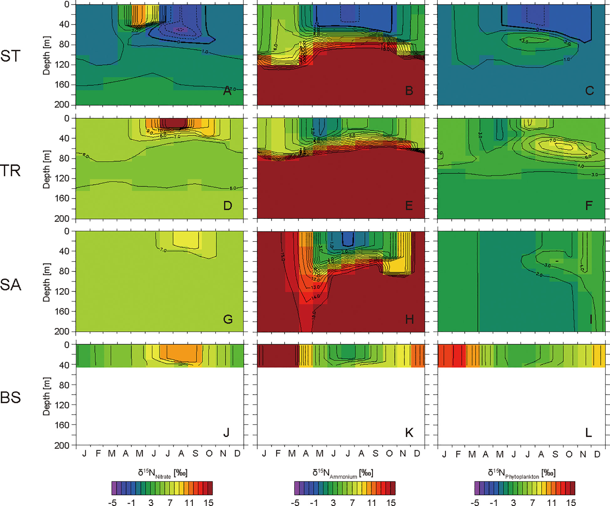
Figure 5 Seasonal cycles of simulated δ¹⁵N values of nitrate, ammonium, and phytoplankton in the layers at 0−200 m at the western subtropical North Pacific site ST (A−C), the Kuroshio–Oyashio transition zone site TR (D−F), the western subarctic North Pacific site SA (G−I), and the Bering Strait region site BS (J−L).

At TR, the simulated δ¹⁵N_Nitrate value in the surface layer is 6.2‰ in February (Figure 5D). The value increases to 17.0‰ in August, and then decreases gradually as the surface mixed layer deepens. The nitrate is slightly depleted in ¹⁵N in the layers at depths of 40−140 m. The simulated ammonium in the surface layer is more depleted in ¹⁵N than the nitrate from March to November, and the minimum value is 0.8‰ in May (Figure 5E). The ammonium is enriched in ¹⁵N from September to February, and the maximum value is 7.8‰ in February. The simulated δ¹⁵N_{Phytoplankton} value is 3.6‰ in the surface layer during the bloom period in June (Figure 5F). The phytoplankton in the surface layer has a minimum δ¹⁵N value of 1.9‰ in May, and is subsequently enriched in ¹⁵N to July and is depleted in ¹⁵N to February as with the seasonal nitrate cycle. The phytoplankton is enriched in ¹⁵N and >5.0‰ in the layers at depths of 30−90 m from July to January.

At SA, the simulated δ¹⁵N_Nitrate value in the surface layer is 6.3‰ in February (Figure 5G), increases to 8.5‰ in August, and then decreases gradually as the surface mixed layer deepens. The seasonal variation in SA is similar to that in TR, although the amplitude is smaller. The simulated ammonium in the surface layer is more depleted in ¹⁵N than nitrate from May to October, and the minimum value is −0.4‰ in July (Figure 5H). Subsequently, the ammonium is enriched in ¹⁵N with a maximum value of 16.8‰ in December. The simulated δ¹⁵N_{Phytoplankton} value is 1.4‰ in the surface layer during the bloom period in June and increases gradually to 4.2‰ in November (Figure 5I).

At BS, the simulated δ¹⁵N_Nitrate value in the surface layer is 3.7‰ in January (Figure 5J). The value increases to 10.8‰ in August, and then decreases gradually as the surface mixed layer deepens. The simulated ammonium in the surface layer is more depleted in ¹⁵N than nitrate from May to October, and the minimum value is 2.4‰ in July (Figure 5K). Subsequently, the ammonium is enriched in ¹⁵N with a maximum value of 17.9‰ in February. The simulated δ¹⁵N_{Phytoplankton} values are 3.2‰ and 4.2‰ in the surface layer during bloom periods in June and August, respectively, and the value increases gradually to 13.6‰ in February (Figure 5L).

4 Discussion

4.1 Western subtropical North Pacific

The western subtropical North Pacific is characterized as an oligotrophic, low-productivity ocean (Figure 2). Active N₂ fixation occurs in the model due to nitrate depletion in the surface water throughout the year (Figure 6). The simulated annual mean δ¹⁵N_{Phytoplankton} value in the euphotic layer at ST is 0.6‰, which is the lowest value among the selected sites. The diazotrophs take up N₂ gas, the δ¹⁵N value of which is 0.0‰, and are remineralized to ammonium and nitrate. The phytoplankton takes up the ¹⁵N-depleted ammonium and nitrate, and consequently is depleted in ¹⁵N.

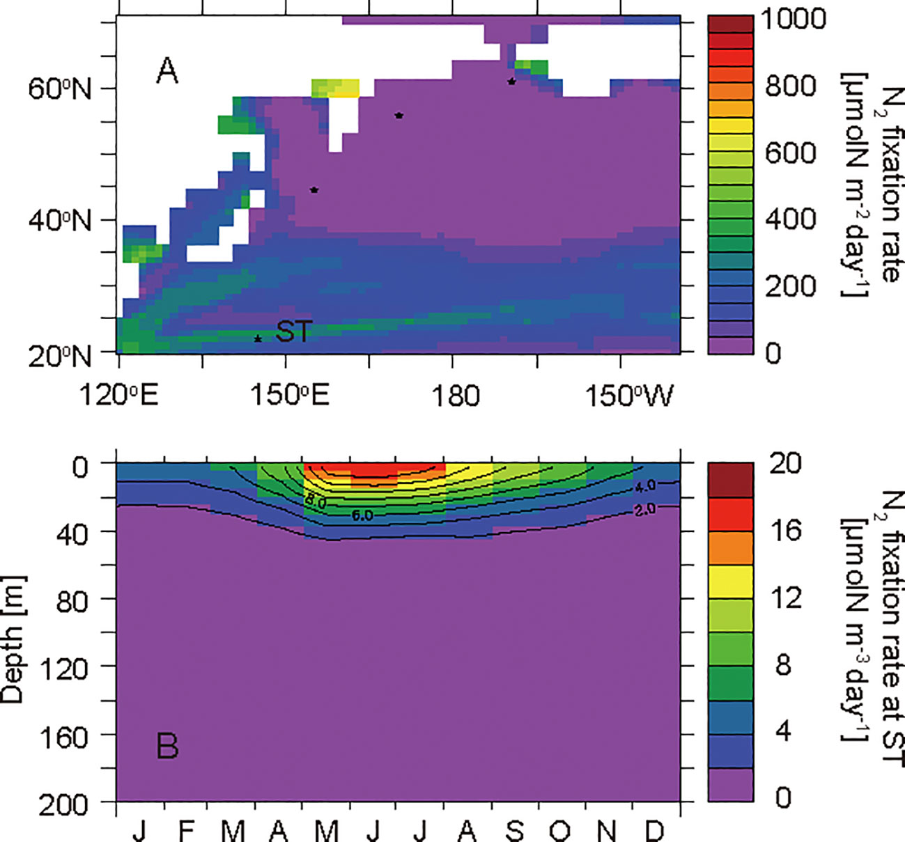
Figure 6 Horizontal distribution of annual mean N₂ fixation rates that were depth-integrated throughout the water column (A) and seasonal cycle of N₂ fixation rates in the layers at 0−200 m at the western subtropical North Pacific site ST (B).

In winter, a small amount of nitrate is present in the surface water (Figure 4A). In early spring, the phytoplankton consumes the nitrate with an isotopic fractionation of 5‰ (Table 2). Therefore, the nitrate in the surface water is enriched in ¹⁵N at the end of the small bloom (Figure 5A). In summer, the nitrate is completely consumed in the surface water, and the diazotrophs begin to take up N₂ actively (Figure 6B). N₂ fixation depletes ¹⁵N in ammonium, nitrate, and phytoplankton in the surface water (Figures 5A−C).

Ammonium is produced by remineralization of PON, and is consumed by phytoplankton assimilation in the euphotic layer and by nitrification below the euphotic layer. As such, ammonium is accumulated at the bottom of the euphotic layer from spring to autumn (Figure 4B). The isotopic fractionation effect of ammonium assimilation by phytoplankton is as small as 0‰, and that of nitrification is as large as 14‰ (Table 2). As such, the ¹⁵N enrichment of ammonium increases with depth (Figure 5B). The ¹⁵N-enriched ammonium in the subsurface water is supplied to the surface layer by the deepening of the mixed layer from autumn to winter.

4.2 Oyashio−Kuroshio transition zone

The Oyashio−Kuroshio transition zone in the western North Pacific is characterized as high-productivity ocean (Figure 2). The annual nitrate supply to the surface water is much higher than that at ST (Figures 4A, D), and the phytoplankton growth is limited only by nitrogen in the surface water (Figure 7A). Therefore, primary productivity is relatively high and phytoplankton exhausts nitrate in the surface water in summer. The simulated annual mean δ¹⁵N_{Phytoplankton} value in the euphotic layer at TR is 3.9‰, which is a high value among the selected sites.

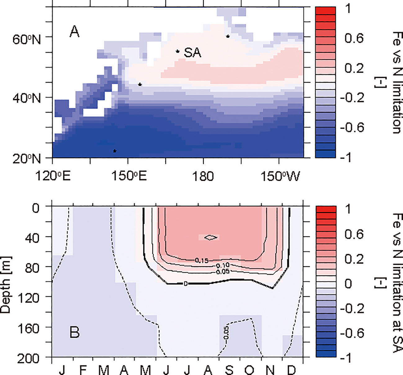
Figure 7 Horizontal distribution of the annual mean nutrient limitation (iron versus nitrogen) for phytoplankton in the surface layer (A) and the seasonal cycle in the layers at 0−200 m at the western subarctic North Pacific site SA (B). The values were calculated from a nutrient-dependent term in the phytoplankton growth rate equation. Red shows the area where phytoplankton growth is limited by iron concentrations. Blue shows the area where phytoplankton growth is limited by nitrate and ammonium concentrations.

In winter, the nitrate in the surface water reaches its maximum concentration during the year due to winter convective mixing (Figure 4D). In spring, phytoplankton starts to consume the nitrate with an associated isotopic fractionation. Therefore,¹⁵N enrichment of nitrate in the surface water proceeds toward summer (Figure 5D). In summer, nitrate is exhausted in the surface water and the maximum δ¹⁵N_Nitrate value during the year is reached. Because phytoplankton actively assimilates nitrate, the seasonal variation in δ¹⁵N_{Phytoplankton} is synchronized with that in δ¹⁵N_Nitrate in the surface water (Figures 5D, F).

Ammonium accumulation is high in the subsurface water from spring to autumn due to active remineralization of PON (Figure 4E). The large isotopic fractionation of nitrification causes ¹⁵N enrichment in ammonium and ¹⁵N depletion in nitrate in the subsurface water (Figures 5D, E). The ¹⁵N enrichment in phytoplankton in the subsurface water from summer to autumn is attributed to the phytoplankton assimilating ¹⁵N-enriched ammonium (Figure 5F).

4.3 Western subarctic North Pacific

The western subarctic North Pacific is characterized as a high-nutrient low-chlorophyll ocean (Figure 2; e.g., Nishioka et al., 2020). Phytoplankton is affected by iron limitation and cannot assimilate all nitrate in the surface water in summer (Figure 7). The simulated annual mean δ¹⁵N_{Phytoplankton} value in the euphotic layer at SA is 2.2‰, which is a low value among the selected sites. The low utilization of the surface nitrate pool by phytoplankton causes ¹⁵N depletion in phytoplankton at SA, as suggested by Yoshikawa et al. (2018).

In winter, nitrate in the surface water reaches its maximum concentration during the year due to winter convective mixing (Figure 4G). In spring, phytoplankton starts to consume the nitrate with an associated isotopic fractionation, and thus the nitrate in the surface water is gradually enriched in ¹⁵N toward summer (Figure 5G). Because the nitrate assimilation by phytoplankton is limited by iron from May to December (Figure 7B), the minimum nitrate concentration and the maximum δ¹⁵N_Nitrate value at SA are much higher and much lower than those at TR, respectively.

The ammonium is accumulated in the subsurface water from spring to autumn due to remineralization of PON (Figure 4H). As found at ST and TR, the ammonium is enriched in ¹⁵N with depth at SA (Figure 5H). The ¹⁵N-enriched ammonium in the subsurface water is supplied to the surface layer by the deepening of the mixed layer. From autumn to winter, the ammonium at SA is much more enriched in ¹⁵N than that at TR. Because the phytoplankton assimilates the extremely ¹⁵N-enriched ammonium (Figure 5I), the phytoplankton in the surface water from autumn to winter is the most enriched in ¹⁵N during the year.

4.4 Bering Strait region

The Bering Strait region is characterized by a highly productive coastal ocean (Figure 2). The high sinking PON flux reaching the seafloor causes active benthic denitrification (Figure 8A). The depth of the ocean floor is only 41 m, and thus nitrification is inhibited by light in most of the water column (Figure 8B), and ammonium is not completely oxidized to nitrate throughout the year. The simulated annual mean δ¹⁵N_{Phytoplankton} value in the euphotic layer at BS is 6.7‰, which is the highest value among the selected sites. The ¹⁵N enrichment in phytoplankton is attributed to the uptake of highly-concentrated ¹⁵N-enriched ammonium caused by partial nitrification and the removal of ¹⁵N-depleted nitrate by benthic denitrification, as suggested by Granger et al. (2011).

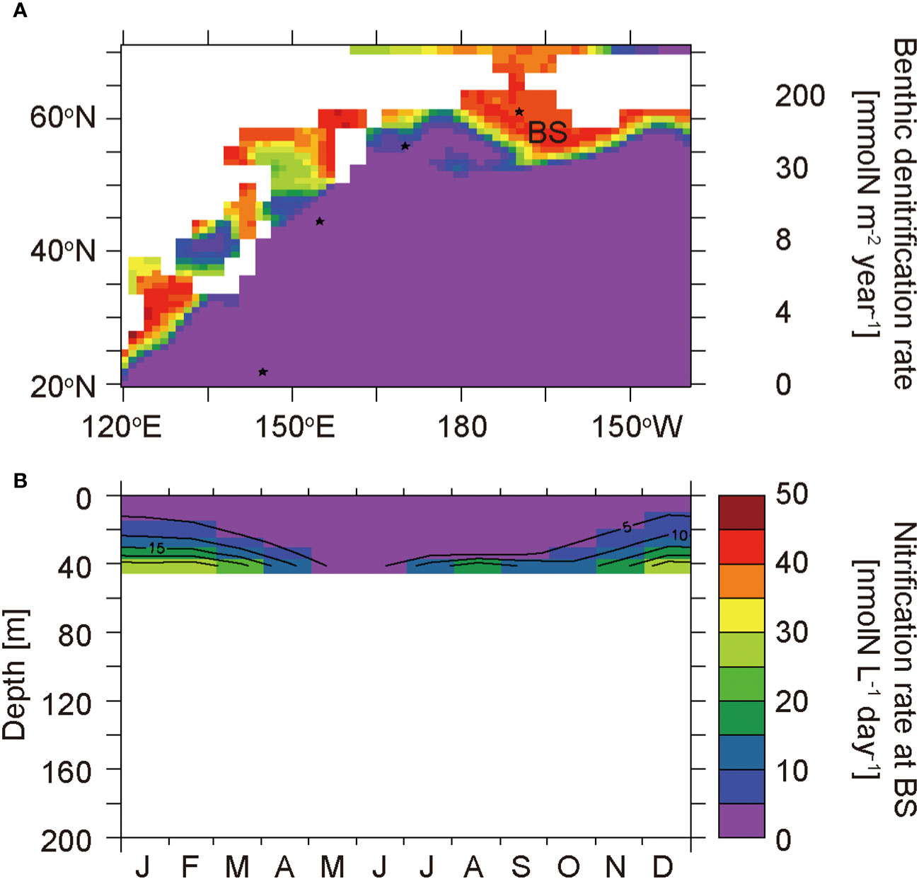
Figure 8 Horizontal distribution of benthic denitrification rates (A) and the seasonal cycle of nitrification rates in the layers at 0−41 m at the Bering Strait region site BS (B).

In winter, nitrate in the surface water reaches its maximum concentration during the year (Figure 4J). In spring, phytoplankton starts to consume nitrate with an associated isotopic fractionation, and consequently the nitrate in the surface water is enriched in ¹⁵N toward summer (Figure 5J). The δ¹⁵N_Nitrate value in winter at BS is much lower than that at TR and SA due to incomplete nitrification with a large isotopic fractionation. The ¹⁵N-depleted nitrate is removed from the benthic water by benthic denitrification after the bloom in June. The δ¹⁵N_Nitrate value in the benthic water increases slightly with the decrease in nitrate concentration (Figures 4J and 5J) because the isotope fractionation during the benthic denitrification is small as 1‰ (Table 2).

Ammonium is not completely consumed by nitrification due to photo-inhibition throughout the water column, and thus ammonium accumulation is high in the benthic layer (Figures 4K and 8B). The ammonium is enriched in ¹⁵N due to partial nitrification with a large isotopic fractionation. ¹⁵N-enriched ammonium in the benthic water is supplied to the surface layer by the deepening of the mixed layer from autumn to winter and is gradually consumed by nitrification. As such, the δ¹⁵N_Ammonium value in the surface water is high and varies drastically. As the phytoplankton takes up the ammonium throughout the year, the δ¹⁵N_{Phytoplankton} value at BS is high and is synchronized with the cycle of the δ¹⁵N_Ammonium value (Figures 5K, L).

5 Summary

A seamless nitrogen isoscape of phytoplankton in the western North Pacific was created by using a marine nitrogen isotope model. The simulated annual average of δ¹⁵N_{Phytoplankton} values in the euphotic layer ranged between −2.9‰ and 17.2‰ in the western North Pacific. Four distinctive sites were selected for discussion. At ST in the western subtropical North Pacific, the δ¹⁵N_{Phytoplankton} value was as low as 0.6‰. The depletion in ¹⁵N of phytoplankton was attributed to N₂ fixation. At TR in the Oyashio−Kuroshio transition zone, the δ¹⁵N_{Phytoplankton} value was as high as 3.9‰. The ¹⁵N enrichment of phytoplankton was attributed to the high utilization of the surface nitrate pool by phytoplankton. At SA in the western subarctic North Pacific, the δ¹⁵N_{Phytoplankton} value was as low as 2.1‰. The depletion of ¹⁵N in phytoplankton was attributed to the low utilization of the surface nitrate pool by phytoplankton due to iron limitation. At BS, the δ¹⁵N_{Phytoplankton} value was as high as 6.7‰. The enrichment of ¹⁵N in phytoplankton was attributed to partial nitrification with benthic denitrification.

The δ¹⁵N_{Phytoplankton} value showed a characteristic seasonal variation at each site. At ST, the δ¹⁵N_{Phytoplankton} value varied from −1.1‰ to 1.3‰. The nitrate and ammonium were exhausted and N₂ fixation occurred throughout the year. Because the N₂ and recycled ammonium supported most of the production, the seasonal variation in δ¹⁵N_{Phytoplankton} at ST was as small as 2.4‰. At TR, the δ¹⁵N_{Phytoplankton} values varied from 1.9‰ to 7.1‰. Convective mixing supplied nitrate from the subsurface to the surface in winter. Because phytoplankton consumes nitrate almost completely with an associated isotopic fractionation, nitrate was enriched greatly in ¹⁵N from 6.2‰ to 17.0‰, and subsequently phytoplankton was also enriched greatly in ¹⁵N. The high utilization of nitrate by phytoplankton caused the large seasonal variation in δ¹⁵N_{Phytoplankton} values of 5.2‰. At SA, the δ¹⁵N_{Phytoplankton} values varied from 1.3‰ and 4.2‰. The phytoplankton was affected by iron limitation and could not consume nitrate completely. The low utilization of nitrate by phytoplankton causes the relatively small seasonal variation in δ¹⁵N_{Phytoplankton} values of 2.9‰. At BS, the δ¹⁵N_{Phytoplankton} values varied from 3.2‰ and 13.6‰. The ammonium concentration was extremely high throughout the year due to partial nitrification. As nitrification proceeded gradually from autumn to winter with a large isotopic fractionation, ammonium was greatly enriched in ¹⁵N from 2.5‰ to 17.9‰. Because phytoplankton assimilates the ammonium, the seasonal variation in δ¹⁵N_{Phytoplankton} values at BS was as large as 10.4‰.

The annual mean δ¹⁵N_{Phytoplankton} value had sufficient spatial variations (e.g., 0.6‰ at ST, 3.9‰ at TR, 2.1‰ at SA, and 6.7‰ at BS) for iso-logging studies in the western North Pacific compared with the analytical errors of the δ¹⁵N_Base values of fish (1σ< ± 0.8‰) (Matsubayashi et al., 2017; Matsubayashi et al., 2020; Harada et al., 2022). The seasonal variability of δ¹⁵N_{Phytoplankton} reached 5.2‰ at TR and 10.4‰ at BS, which were greater than the spatial variability in the western North Pacific. To trace the movement of fish whose habitat is expected to include those areas, the seasonal variations of the nitrogen isoscape should be considered carefully.

Both δ¹⁵N_Base values of fish and a nitrogen isoscape of phytoplankton are needed for iso-logging studies. The estimation of δ¹⁵N_Base values requires the δ¹⁵N measurement of amino acids to correct for ¹⁵N-enrichment of ~3‰ per trophic position of the δ¹⁵N values of bulk nitrogen of fish (Matsubayashi et al., 2017; Matsubayashi et al., 2020; Harada et al., 2022). However, because the δ¹⁵N measurement of amino acids still takes much time and effort, there have been a few previous studies of the δ¹⁵N values of amino acids. Nitrogen isoscapes of diet (zooplankton or small fish) using a nitrogen isotope model, including higher-trophic-level organisms, will advance iso-logging studies.

Data availability statement

The raw data supporting the conclusions of this article will be made available by the authors, without undue reservation.

Author contributions

CY: Conceptualization, Data curation, Formal Analysis, Funding acquisition, Methodology, Project administration, Software, Validation, Visualization, Writing – original draft, Writing – review & editing. MS: Conceptualization, Methodology, Software, Writing – review & editing. AY: Conceptualization, Methodology, Software, Writing – review & editing. AO: Conceptualization, Methodology, Software, Writing – review & editing. NO: Conceptualization, Funding acquisition, Project administration, Supervision, Writing – review & editing.

Funding

The author(s) declare financial support was received for the research, authorship, and/or publication of this article. We acknowledge support from JSPS KAKENHI Grants 19H04247, 19KK0293, 19K22917 20KK0165, and 21H03579. MS acknowledges support from JSPS KAKENHI Grants 18H04129 and 19H04246.

Acknowledgments

We thank D.M. Sigman, P.A. Rafter, an reviewer, and the editor for their valuable comments, and D. Marconi for suggestions about compiling the D₁₅N_Nitrate data. The simulations with a nitrogen isotope model were performed using the Earth Simulator (ES4) at JAMSTEC. This study is partially supported by the Cooperative Research Activities of Collaborative Use of Computing Facility of the Atmosphere and Ocean Research Institute, the University of Tokyo. The analysis and graphics in this paper employed the Ferret program of NOAA’s Pacific Marine Environmental Laboratory.

Conflict of interest

The authors declare that the research was conducted in the absence of any commercial or financial relationships that could be construed as a potential conflict of interest.

Publisher’s note

All claims expressed in this article are solely those of the authors and do not necessarily represent those of their affiliated organizations, or those of the publisher, the editors and the reviewers. Any product that may be evaluated in this article, or claim that may be made by its manufacturer, is not guaranteed or endorsed by the publisher.

Supplementary material

The Supplementary Material for this article can be found online at: https://www.frontiersin.org/articles/10.3389/fmars.2024.1294608/full#supplementary-material

References

Bianchi D., Dunne J. P., Sarmiento J. L., Galbraith E. D. (2012). Data-based estimates of suboxia, denitrification, and N2O production in the ocean and their sensitivities to dissolved O2. Global Biogeochem. Cycles 26, GB2009. doi: 10.1029/2011GB004209
Bohlen L., Dale A. W., Wallmann K. (2012). Simple transfer functions for calculating benthic fixed nitrogen losses and C:N:P regeneration ratios in global biogeochemical models. Global Biogeochem. Cycles 26, GB3029. doi: 10.1029/2011GB004198
Coles V. J., Hood R. R. (2007). Modeling the impact of iron and phosphorus limitations on nitrogen fixation in the Atlantic Ocean. Biogeoscienced 4, 455–497. doi: 10.5194/bg-4-455-2007
Coles V. J., Hood R. R., Pascual M., Capone D. G. (2004). Modeling the effects of Trichodesmium and nitrogen fixation in the Atlantic Ocean. J. Geophys. Res. 109, C06007. doi: 10.01029/02002JC001754
DeVries T., Deutsch C., Rafter P. A., Primeau F. (2013). Marine denitrification rates determined from a global 3-D inverse model. Biogeosciences 10, 2481–2496. doi: 10.5194/bg-10-2481-2013
FAO (2022). “The state of world fisheries and aquaculture 2022,” in Towards Blue Transformation (Rome, Italy: Food and Agriculture Organization of the United Nations (FAO)). doi: 10.4060/cc0461en
Fripiat F., Marconi D., Rafter P. A., Sigman D. M., Altabet M. A., Bourbonnais A., et al. (2021). Compilation of nitrate δ15N in the ocean. PANGAEA. doi: 10.1594/PANGAEA.936484
Garcia H. E., Weathers K., Paver C. R., Smolyar I., Boyer T. P., Locarnini R. A., et al. (2019). World Ocean Atlas 2018, Volume 4: Dissolved Inorganic Nutrients (phosphate, nitrate and nitrate+nitrite, silicate). A. Mishonov Tech. Ed.; NOAA Atlas NESDIS 84, 35.
Granger J., Prokopenko M. G., Sigman D. M., Mordy C. W., Morse Z. M., Morales L. V., et al. (2011). Coupled nitrification-denitrification in sediment of the eastern Bering Sea shelf leads to 15N enrichment of fixed N in shelf waters. J. Geophys. Res. 116, C11006. doi: 10.1029/2010JC006751
Granger J., Sigman D. M., Lehmann M. F., Tortell P. D. (2008). Nitrogen and oxygen isotope fractionation during dissimilatory nitrate reduction by denitrifying bacteria. Limnol. Oceanogr. 53 (6), 2533–2545. doi: 10.4319/lo.2008.53.6.2533
Granger J., Sigman D. M., Rohde M. M., Maldonado M. T., Tortell P. D. (2010). N and O isotope effects during nitrate assimilation by unicellular prokaryotic and eukaryotic plankton cultures. Geochim. Cosmochim. Acta 74, 1030–1040. doi: 10.1016/j.gca.2009.10.044
Hajima T., Watanabe M., Yamamoto A., Tatebe H., Noguchi M. A., Abe M., et al. (2020). Development of the MIROC-ES2L Earth system model and the evaluation of biogeochemical processes and feedbacks. Geosci. Model. Dev. 13, 2197–2244. doi: 10.5194/gmd-13-2197-2020
Hanselman D. H., Heifetz J., Echave K. B., Dressel S. C. (2015). Move it or lose it: movement and mortality of sablefish tagged in Alaska. Can. J. Fisheries Aquat. Sci. 72, 238–251. doi: 10.1139/cjfas-2014-0251
Harada Y., Ito S., Ogawa N. O., Yoshikawa C., Ishikawa N. F., Yoneda M., et al. (2022). Compound-specific nitrogen isotope analysis of amino acids in eye lenses as a new tool to reconstruct the geographic and trophic histories of fish. Front. Mar. Sci. 8. doi: 10.3389/fmars.2021.796532
Hays G. C., Ferreira L. C., Sequeira A. M., Meekan M. G., Duarte C. M., Bailey H., et al. (2016). Key questions in marine megafauna movement ecology. Trends Ecol. Evol. 31, 463–475. doi: 10.1016/j.tree.2016.02.015
Hood R. R., Bates N. R., Capone D. G., Olson D. B. (2001). Modeling the effect of nitrogen fixation on carbon and nitrogen fluxes at BATS. Deep-Sea Res. II 48, 1609–1648. doi: 10.1016/S0967-0645(00)00160-0
Hood R. R., Coles V. J., Capone D. G. (2004). Modeling the distribution of Trichodesmium and nitrogen fixation in the Atlantic Ocean. J. Geophys. Res. 109, C06006. doi: 10.1029/2002JC001753
Letscher R. T., Hansell D. A., Carlson C. A., Lumpkin R., Knapp A. N. (2013). Dissolved organic nitrogen in the global surface ocean: Distribution and fate, Global Biogeochem. Cycles 27, 141–153. doi: 10.1029/2012GB004449
Liu K.-K., Kao S.-J., Chiang K.-P., Gong G.-C., Chang J., Cheng J.-S., et al. (2013). Concentration dependent nitrogen isotope fractionation during ammonium uptake by phytoplankton under an algal bloom condition in the Danshuei estuary, northern Taiwan. Mar. Chem. 157, 242–252. doi: 10.1016/j.marchem.2013.10.005
Lowerre-Barbieri S. K., Kays R., Thorson J. T., Wikelski M. (2019). The ocean’s movescape: fisheries management in the bio-logging decade, (2018–2028). ICES J. Mar. Sci. 76, 477–488. doi: 10.1093/icesjms/fsy211
Matsubayashi J., Kimura K., Ohkouchi N., Ogawa N. O., Ishikawa N. F., Chikaraishi Y., et al. (2022). Using geostatistical analysis for simultaneous estimation of isoscapes and ontogenetic shifts in isotope ratios of highly migratory marine fish. Front. Mar. Sci. 9. doi: 10.3389/fmars.2022.1049056
Matsubayashi J., Osada Y., Tadokoro K., Abe Y., Yamaguchi A., Shirai K., et al. (2020). Tracking long-distance migration of marine fishes using compound-specific stable isotope analysis of amino acids. Ecol. Lett. 23, 881–890. doi: 10.1111/ele.13496
Matsubayashi J., Saitoh Y., Osada Y., Uehara Y., Habu J., Sasaki T., et al. (2017). Incremental analysis of vertebral centra can reconstruct the stable isotope chronology of teleost fishes. Methods Ecol. Evol. 8, 1755–1763. doi: 10.1111/2041-210X.12834
McMahon K. W., Hamady L., Thorrold S. R. (2013). A review of ecogeochemistry approaches to estimating movements of marine animals. Limnol. Oceanogr. 58, 697–714. doi: 10.4319/lo.2013.58.2.0697
Minagawa M., Wada E. (1984). Stepwise enrichment of 15N along food chains: Further evidence and the relation between d15N and animal age. Geochim. Cosmochim. Acta 48, 1135–1140. doi: 10.1016/0016-7037(84)90204-7
Minagawa M., Wada E. (1986). Nitrogen isotope ratio of red tide organisms in the East China Sea: A characterization of biological nitrogen fixation. Mar. Chem. 19, 245–259. doi: 10.1016/0304-4203(86)90026-5
Montoya J. P., McCarthy J. J. (1995). Isotopic fractionation during nitrate uptake by phytoplankton grown in continuous culture. J. Plankton Res. 17, 439–464. doi: 10.1093/plankt/17.3.439
Nishioka J., Obata H., Ogawa H., Ono K., Yamashita Y., Lee K., et al. (2020). Subpolar marginal seas fuel the North Pacific through the intermediate water at the termination of the global ocean circulation. Proc. Natl. Acad. Sci. 117 (23), 202000658–202000658. doi: 10.1073/pnas.2000658117
Oka A., Kato S., Hasumi H. (2008). Evaluating effect of ballast mineral on deep-ocean nutrient concentration by using an ocean general circulation model. Global Biogeochem. Cycles 22, GB3004. doi: 10.1029/2007GB003067
O’Reilly J. E., Maritorena S., Mitchell B. G., Siegal D. A., Carder K. L., Garver S. A., et al. (1998). Ocean color chlorophyll algorithms for SeaWiFS. J. Geophys. Res. 103, 24937–24953. doi: 10.1029/98JC02160
Rafter P., Bagnell A., DeVries T., Marconi D. (2019). Compiled dataset consisting of published and unpublished global nitrate d15N measurements from from 1975-2018. Biol. Chem. Oceanogr. Data Manage. Office. doi: 10.1575/1912/bco-dmo.768627.1
Schmittner A., Oschlies A., Matthews H. D., Galbraith E. D. (2008). Future changes in climate, ocean circulation, ecosystems and biogeochemical cycling simulated for a business-as-usual CO2 emission scenario until year 4000 AD. Global Biogeochem. Cycles 22, GB1013. doi: 10.1029/2007GB002953
Shigemitsu M., Gruber N., Oka A., Yamanaka Y. (2016). Potential use of the N2/Ar ratio as a constraint on the oceanic fixed nitrogen loss. Global Biogeochem. Cycles 30, 576–594. doi: 10.1002/2015GB005297
Shigemitsu M., Yamamoto A., Oka A., Yamanaka Y. (2017). One possible uncertainty in CMIP5 projections of low-oxygen water volume in the Eastern Tropical Pacific. Global Biogeochem. Cycles 31, 804–820. doi: 10.1002/2016GB005447
Somes C., Oschlies J. A., Schmittner A. (2013). Isotopic constraints on the pre-industrial oceanic nitrogen budget. Biogeosciences 10, 5889–5910. doi: 10.5194/bg-10-5889-2013
Somes C. J., Schmittner A., Galbraith E. D., Lehmann M. F., Altabet M. A., Montoya J. P., et al. (2010). Simulating the global distribution of nitrogen isotopes in the ocean. Global Biogeochem. Cycles 24, GB4019. doi: 10.1029/2009GB003767
Somes C. J., Schmittner A., Muglia J., Oschlies A. (2017). A three-dimensional model of the marine nitrogen cycle during the last glacial maximum constrained by sedimentary isotopes. Front. Mar. Sci. 4. doi: 10.3389/fmars.2017.00108
Tesdal J. E., Galbraith E. D., Kienast M. (2013). Nitrogen isotopes in bulk marine sediment: linking seafloor observations with subseafloor records. Biogeosciences 10, 101–118. doi: 10.5194/bg-10-101-2013
Thorson J. T., Jannot J., Somers K., Punt A. (2016). Using spatio-temporal models of population growth and movement to monitor overlap between human impacts and fish populations. J. Appl. Ecol. 54, 577–587. doi: 10.1111/1365-2664.12664
Tzadik O. E., Curtis J. S., Granneman J. E., Kurth B. N., Pusack T. J., Wallace A. A., et al. (2017). Chemical archives in fishes beyond otoliths: a review on the use of other body parts as chronological recorders of microchemical constituents for expanding interpretations of environmental, ecological, and life-history changes. Limnol. Oceanogr.: Methods 15, 238–263. doi: 10.1002/lom3.10153
Vecchio J. L., Peebles E. B. (2020). Spawning origins and ontogenetic movements for demersal fishes: An approach using eye-lens stable isotopes. Estuar. Coast. Shelf. Sci. 246, 107047. doi: 10.1016/j.ecss.2020.107047
Wada E., Hattori A. (1978). Nitrogen isotope effects in the assimilation of inorganic nitrogenous compounds by marine diatoms. Geomicrobiol. J. 1, 85–101. doi: 10.1080/01490457809377725
Watanabe S., Hajima T., Sudo K., Nagashima T., Takemura T., Okajima H., et al. (2011). MIROC-ESM 2010: Model description and basic results of CMIP5-20c3m experiments, Geosci. Model. Dev. 4, 845–872. doi: 10.5194/gmd-4-845-2011
Yamamoto A., Abe-Ouchi A., Ohgaito R., Ito A., Oka A. (2019). Glacial CO2 decrease and deep-water deoxygenation by iron fertilization from glaciogenic dust. Climate Past 15 (3), 981–996. doi: 10.5194/cp-15-981-2019
Yoshikawa C., Abe H., Aita M. N., Breider F., Kuzunuki K., Toyoda S., et al. (2016). Insight into nitrous oxide production processes in the western North Pacific based on a marine ecosystem isotopomer model. J. Oceanogr. 72 (3), 491–508. doi: 10.1007/s10872-015-0308-2
Yoshikawa C., Coles V. J., Hood R. R., Capone D. G., Yoshida N. (2013). Modeling how surface nitrogen fixation influences subsurface nutrient patterns in the North Atlantic. J. Geophys. Res. Oceans 118, 2520–2534. doi: 10.1002/jgrc.20165
Yoshikawa C., Makabe A., Matsui Y., Nunoura T., Ohkouchi N. (2018). Nitrate isotope distribution in the subarctic and subtropical North Pacific. Geochem. Geophys. Geosystems 19, 2212–2224. doi: 10.1029/2018GC007528
Yoshikawa C., Ogawa N. O., Chikaraishi Y., Makabe A., Matsui Y., Sasai Y., et al. (2022). Nitrogen isotopes of sinking particles reveal the seasonal transition of the nitrogen source for phytoplankton. Geophys. Res. Lett. 49, e2022GL098670. doi: 10.1029/2022GL098670
Keywords: isoscape, nitrogen isotopes, marine nitrogen cycle, nitrogen isotope model, western North Pacific
Citation: Yoshikawa C, Shigemitsu M, Yamamoto A, Oka A and Ohkouchi N (2024) A nitrogen isoscape of phytoplankton in the western North Pacific created with a marine nitrogen isotope model. Front. Mar. Sci. 11:1294608. doi: 10.3389/fmars.2024.1294608
Received: 15 September 2023; Accepted: 03 January 2024;
Published: 22 January 2024.
Edited by:
Paulo Sergio Salomon, Federal University of Rio de Janeiro, BrazilReviewed by:
Hyun Je Park, Gangneung-Wonju National University, Republic of KoreaPatrick Rafter, University of California, Irvine, United States
Copyright © 2024 Yoshikawa, Shigemitsu, Yamamoto, Oka and Ohkouchi. This is an open-access article distributed under the terms of the Creative Commons Attribution License (CC BY). The use, distribution or reproduction in other forums is permitted, provided the original author(s) and the copyright owner(s) are credited and that the original publication in this journal is cited, in accordance with accepted academic practice. No use, distribution or reproduction is permitted which does not comply with these terms.
*Correspondence: Chisato Yoshikawa, yoshikawac@jamstec.go.jp