Not another hillshade: alternatives which improve visualizations of bathymetric data

1 Introduction

Advances in remote sensing technologies in recent decades have allowed an ever-increasing capability to monitor the Earth’s surface - both onshore (Drăguţ and Eisank, 2011; Tarolli, 2014; Telling et al., 2017; Sofia, 2020) and offshore (Lecours et al., 2016; Hughes Clarke, 2018; Micallef et al., 2018; Wölfl et al., 2019). As a result, digital elevation models (hereafter DEMs) have become essential in geoscientific applications. Recent advances in computing and technology facilitate acquisition and processing of large quantities of elevation data and the creation of DEMs in increasingly higher resolutions (Sofia, 2020 and references therein). While the most recent advancements are focused towards quantitative analyses of elevation data and machine learning (Lecours et al., 2016; Maxwell and Shobe, 2022), qualitative analyses are still very important in geomorphological, environmental, archaeological, geographical, and geological studies. In these studies, very often one of the first steps involves the preliminary visual inspection of elevation data which then dictates the selection of the study site and directly impacts the study results. In later stages, a clear visual representation of elevation data is essential for efficiently communicating the results, analyses, and interpretations to the reader. For these reasons, representative and intuitive visualization of elevation data plays an essential role in research- and application-driven studies.

The importance of representative visualization of the Earth’s surface is even more pronounced in offshore (in this manuscript referring to marine, lacustrine and fluvial) environments where visual on-site inspection is rarely possible or very costly, and where the availability and resolution of bathymetric data is very limited compared to elevation data from onshore areas (Weatherall et al., 2015; Mayer et al., 2018; Wölfl et al., 2019). Due to relatively costly acquisition, a great majority of high-resolution bathymetric data is obtained by multibeam sonar in near-shore areas, areas containing important economic resources and at sites intended for larger infrastructural development (Mayer et al., 2018; Wölfl et al., 2019). Due to the relative scarcity of high-resolution offshore elevation data, it is of great importance to extract useful information from bathymetric data to the fullest.

Most commonly, elevation data and morphological features are visualized with the hillshading method in which the lightness or darkness of a surface is determined by the incidence angle between the illumination direction and the surface, resulting in an intuitive representation of the morphology of the Earth’s surface (Kokalj et al., 2011; Zakšek et al., 2011). Some recent publications displaying hillshaded bathymetric data include: Madricardo et al., 2019; Caporizzo et al., 2021; Fabbri et al., 2021; Wu et al., 2021; Aiello and Sacchi, 2022; Li et al., 2022; Piret et al., 2022; Post et al., 2022; Riddick et al., 2022; Sandwell et al., 2022; Streuff et al., 2022; Zheng et al., 2022. Despite the widespread use of the Hillshade, analytical hillshading has inherent limitations due to the directional bias induced by a single light source (Onorati et al., 1992; Smith and Clark, 2005; Zakšek et al., 2011; Kokalj and Somrak, 2019). The two most common problems with hillshading are 1) that morphological features which are parallel to the light source are barely visible (sometimes even invisible), and 2) that directly lit/shaded features are too light/dark to exhibit subtle relief (Zakšek et al., 2011). In order to partially mitigate these limitations, alternative visualizations of bathymetric data and morphological features are being used, among which Slope Gradient prevails by far (some more recent examples include: Walbridge et al., 2018; Watson et al., 2020; Georgiou et al., 2021; Verweirder et al., 2021; Berthod et al., 2022; Lebrec et al., 2022; Manstretta et al., 2022; Puga-Bernabéu et al., 2022). With this method the colour of a surface depends on its steepness. Even though the Slope Gradient visualization is less intuitive than Hillshade (Kokalj et al., 2019), it is still widely used since it is included as a standard function in commonly used GIS software packages. Other visualizations of bathymetric data and morphological features are only used occasionally (Marple and Hurd, 2019; Majcher et al., 2020; Zhou et al., 2022) as they are rarely included in the analytical toolbox of GIS software solutions and require the use of various programming languages for their calculation.

In this paper we present a fresh approach to offshore mapping by exploring the different visualization algorithms provided by the freely available “Relief Visualization Toolbox” software package (hereafter RVT). We assess the suitability of RVT algorithms for visualizing bathymetric data in different settings, resolutions, and regions and try to identify the most suitable algorithms to highlight different natural (i.e. geological) and anthropogenic geomorphic sea-, lake- and riverbed features. To our knowledge, we provide the first summary of the suitability of RVT algorithms for highlighting submerged features. Finally, we try to convince the reader that there are user-friendly simple-to-use alternatives to the Analytical Hillshade that have great potential to more effectively display bathymetric data and allow users to more efficiently communicate their findings and ideas.

2 Methods

2.1 Software

The “Relief Visualization Toolbox” is a freely available software package which was developed by ZRC SAZU and the University of Ljubljana (Kokalj et al., 2011; Zakšek et al., 2011; Kokalj and Somrak, 2019; Kokalj et al., 2019; RVT, 2023). It is compatible with the two most commonly used GIS software solutions and is frequently used in land applications. At the moment, RVT is available as a standalone executable (available at https://www.zrc-sazu.si/en/rvt; last accessed: 22.6.2023), as a plugin for the QGIS GIS software, as a “raster function” for the ArcGIS Pro GIS software, and as a Python package (all three available at https://rvt-py.readthedocs.io/; last accessed: 22.6.2023). For this paper we created the visualizations by utilising the standalone executable, the RVT plugin for QGIS, and the RVT “Raster function” for ArcGIS.

In this work, we focus on the following visualization functions of the RVT Toolbox: “Hillshade” (hereafter HS), “Hillshading from Multiple Directions” (hereafter HSM), “Principal Component Analysis of Hillshading” (hereafter PCAHS), “Simple Local Relief Model” (hereafter SLRM), “Multi-Scale Relief Model” (hereafter MSRM; Orengo and Petrie, 2018), “Sky-View Factor” (hereafter SVF; Zakšek et al., 2011), “Anisotropic SVF” (hereafter ASVF), “Openness – Negative” & “Openness– Positive” (hereafter ONEG and OPOS; Yokoyama et al., 2002), and “Local Dominance” (hereafter LD). All the algorithms used to create the listed visualizations are described in detail in Kokalj et al. (2019) and in Kokalj and Somrak (2019). These references also contain the basic guidelines for setting the algorithm parameters for the creation of individual visualizations. A very basic description of the algorithms is here summarised after Kokalj et al. (2019); Kokalj and Somrak (2019), and RVT (2023): HS – illuminates a surface depending on the incidence angle between the illumination direction and the surface, HSM – a composite image of hillshading from multiple directions, PCAHS – a PCA analysis of hillshaded data from multiple directions, SLRM – a trend-removal algorithm that separates local small-scale features from large-scale landforms, MSRM – as SLRM but at multiple scales, SVF – a graphical representation of the portion of the sky visible from a certain point, ASVF - a modification of SVF which takes into account the directional variability of the brightness of the sky, ONEG - a proxy for diffuse relief illumination resulting in a topography-detrended image based on estimating the mean value of mean nadir value within a defined search radius, OPOS – similar to ONEG but based on estimating the mean value of all zenith angles within a defined search radius, LD - demonstrates how dominant an observer is for a local surrounding area when standing above a certain elevation. For more details the reader is referred to the beforementioned references.

Although “Multi-Scale Topographic Position” and “Slope Gradient” algorithms are also available in the RVT Toolbox, we do not present them in this work. “Multi-Scale Topographic Position” is most commonly used for landscape slope classification (Guisan et al., 1999; De Reu et al., 2013), and is therefore less applicable for visualization and mapping of subtle geomorphic features commonly occurring in bathymetric datasets. On the other hand, “Slope Gradient” is well known and commonly used also in bathymetric applications (as already described in the Introduction), therefore we do not elaborate on it any further in this work.

We tested the suitability of the described algorithms to visualize the following morphologies: narrow linear features with negligible relief, convex linear and elongate features, concave linear and elongate features, linear or curved features with break in slope, circular-rounded convex features, circular-rounded concave features, and features with a corrugated/folded morphology. These general morphologies comprise some of the most common geological, geomorphic, and anthropogenic features that can be found on the sea-, lake- and riverbeds (Table 1).

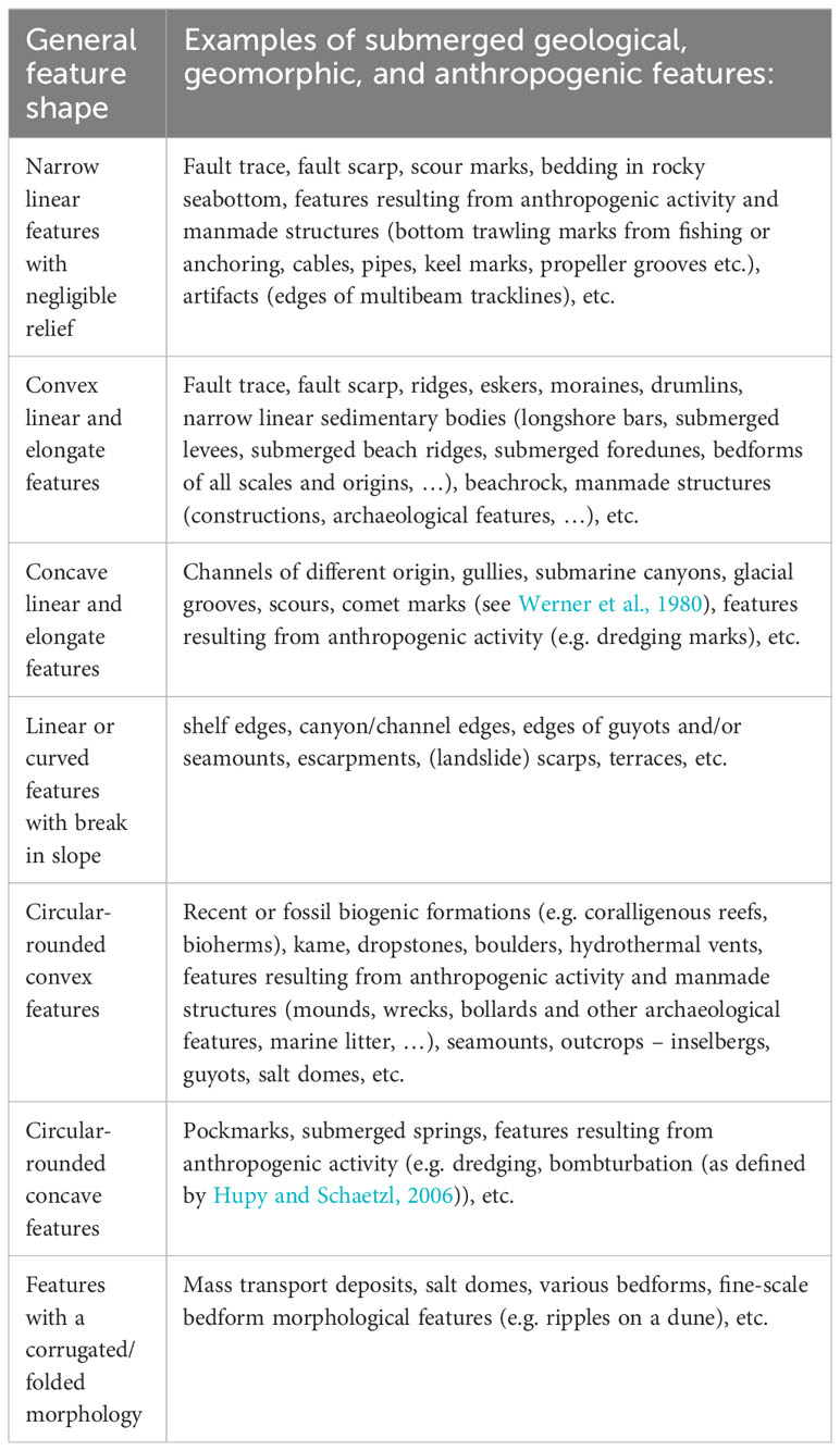
Table 1 Most common sea-, lake- and riverbed morphologies and corresponding examples of geological, geomorphic and anthropogenic features.

2.2 Datasets

In order to try to represent the widest possible variety of bathymetric data, we present results from four different datasets (Figure 1) covering different bathymetric ranges, geological & geographical settings, dataset resolutions and source data types. The datasets are from the Gulf of Trieste, the New England Seamount chain, and from lakes Constance (also Bodensee, Lac de Constance, Lago di Costanza, Lai da Constanza) and Lucerne (also Vierwaldstättersee, Lac des Quatre-Cantons, Lago di Lucerna, Lai dals Quatter Chantuns). Table 2 provides the basic information about the used datasets and lists references describing their geological setting. Datasets for the Gulf of Trieste and lakes Constance and Lucerne were created from multibeam sonar soundings, except in the very shallow areas of the Gulf of Trieste, where singlebeam sonar was also used (Slavec, 2012; Trobec et al., 2017). The source data for the New England Seamount chain dataset is composed of direct and indirect measurements – where sonar soundings are available, they are combined with satellite-derived bathymetry (GEBCO, 2021).

Figure 1 Geographic location of the used bathymetric datasets indicated by dark blue polygons: (A) overview map (EPSG: 4326); (B) inset of the northern Adriatic Sea (EPSG: 3794), (C) inset of Switzerland (EPSG: 2056). Figure was created by using Flanders Marine Institute (2018) and EuroGeographics & UN-FAO (2020) datasets for the seas/oceans extent and administrative boundaries.

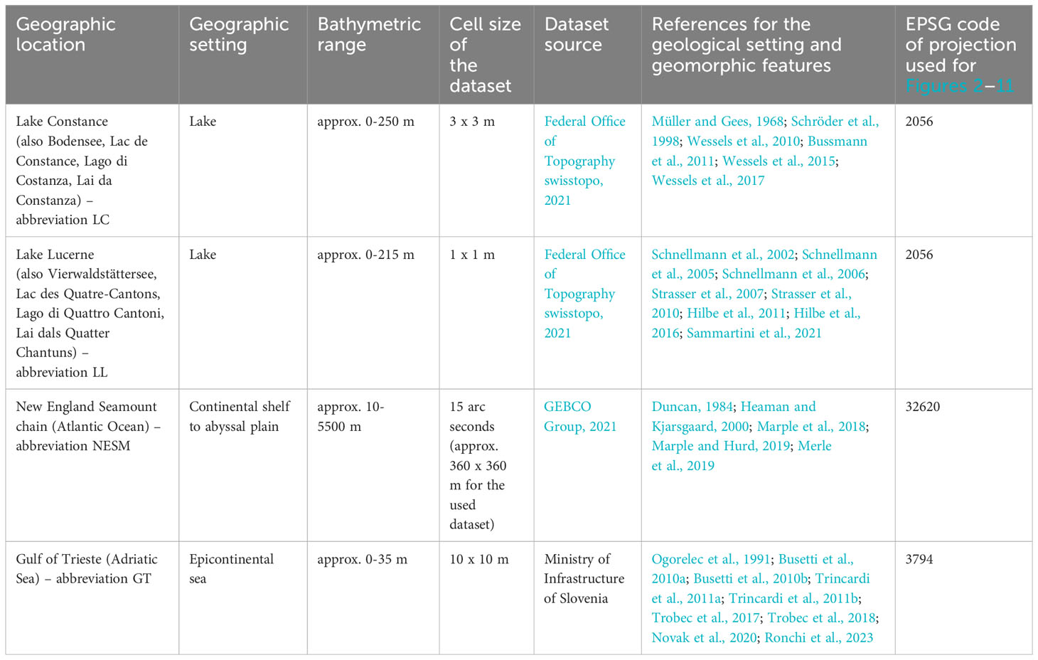
Table 2 Datasets used in this study.

3 Results

This section contains an overview of the visualizations which were created from the four different datasets which were used in this study (Table 2). We show the most striking examples and assess the effectiveness of the different algorithms for highlighting different geomorphic features. We first assess which visualizations are suitable to give a general overview of the bathymetric relief of a research area and then determine which visualizations most effectively highlight the general shapes listed in Table 1. The results of our qualitative assessment are summarized in Table 3 which shows the suitability of the different algorithms for highlighting specific morphological sea-, lake-, and riverbed features.

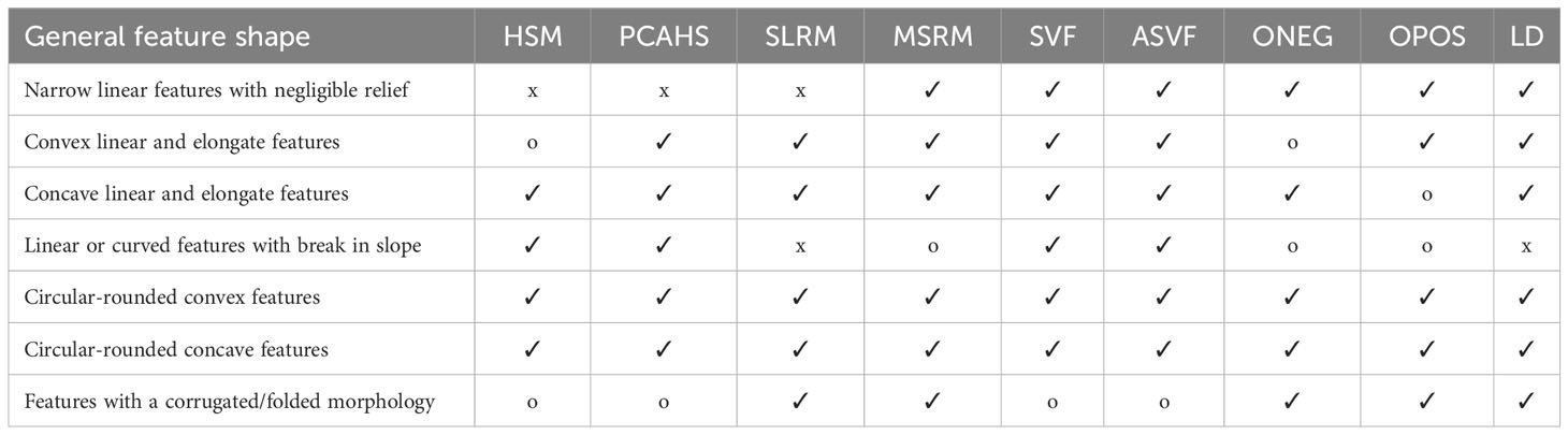
Table 3 Suitability of the different algorithms for highlighting specific morphological features (✓ - very suitable, ο - less suitable, x - not suitable).

The abbreviations which are used in the figure captions refer to the: geographic location of the dataset (abbr. explained in Sect. 2.2 and Table 2), used visualization algorithm (abbr. explained in Sect. 2.1), and the used parameters (where applicable). The abbreviations for the latter are: A - azimuth of illumination (in degrees), An - main direction of anisotropy (in degrees); H - height of illumination source (in degrees), Ve - vertical exaggeration (in multiples), D - number of directions of illumination, R - radius for trend assessment (in pixels), and M[min]-[max] - minimum to maximum search radius (in meters). The different parameters are separated by an underscore symbol.

3.1 General morphology of a research area

In order to create a good overview of the general morphology of a research area, the HSM, PCAHS (Figure 2), MSRM (Figure 3), SVF, and ASVF (Figure 4) algorithms are especially effective. However, the general morphology of the research area (especially in very low- or very high-gradient settings) should be taken into account before using HS or HSM as improperly set parameters can completely obscure the relief (e.g. Figures 2A, C).

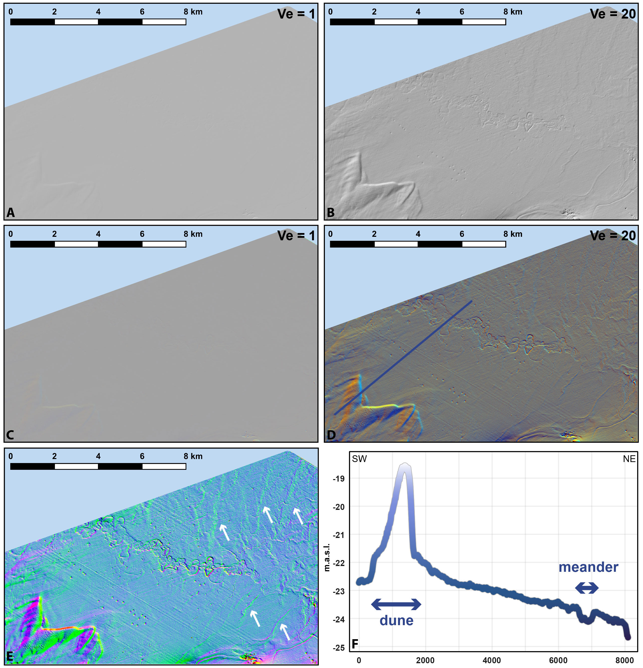
Figure 2 Examples of visualizations in a low-gradient setting (dataset from GT): (A) HS A315_H35_Ve1; (B) HS A315_H35_Ve20; (C) HSM D8_H20_Ve1; (D) HSM D8_H20_Ve20; (E): PCAHS D8_H20_Ve20; (F) example of an elevation profile throughout research area (profile location indicated in (D). Note how at low Ve relief features in A and C are barely visible (e.g. dunes in the SW part of the figure; see Slavec, 2012) or even invisible (e.g. the buried meander belt in the central part of the figure; see Trobec et al., 2017; Novak et al., 2020). White arrows in E indicate some examples of relatively subtle linear convex sedimentary bodies.

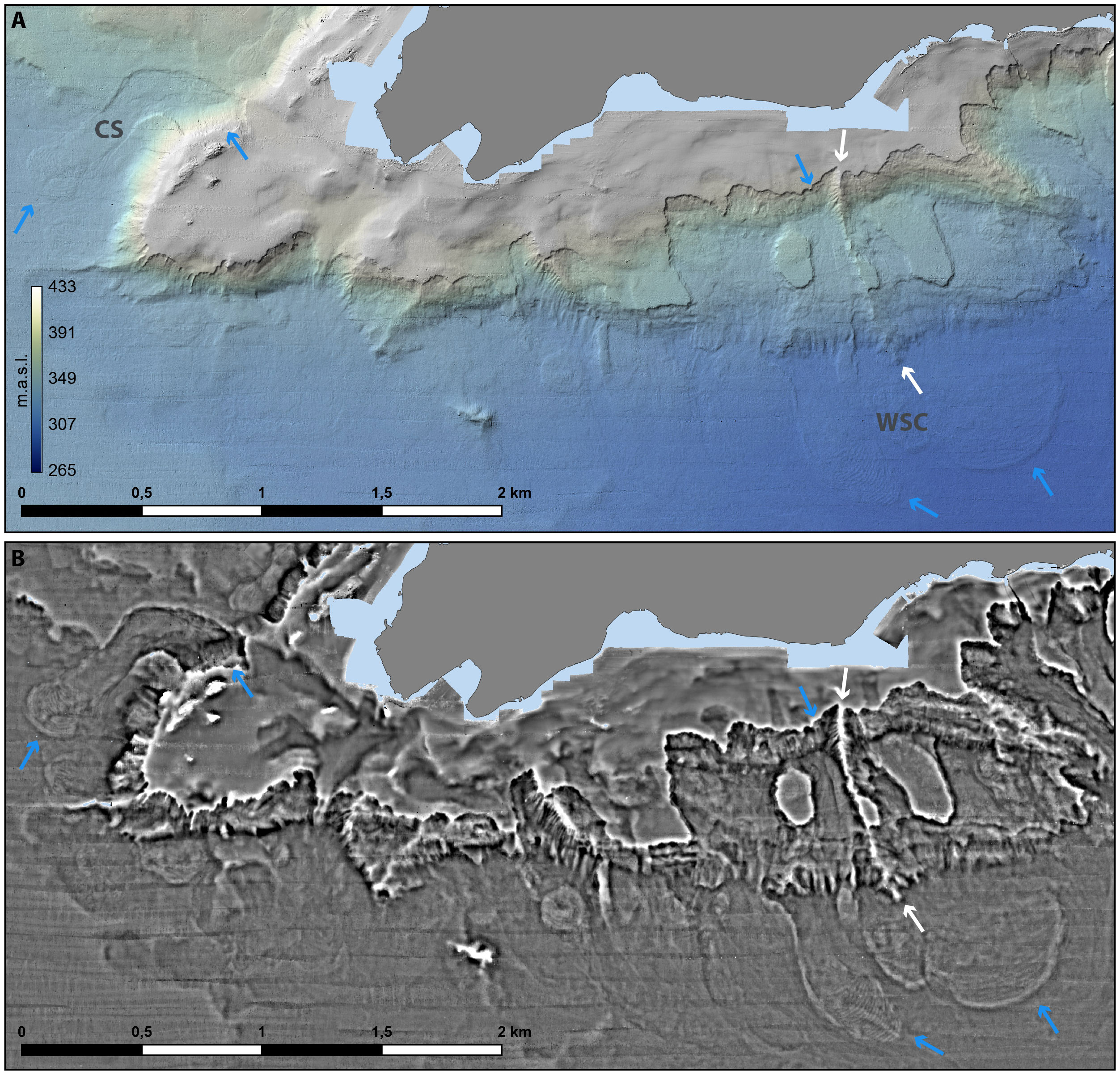
Figure 3 Examples of visualization in a mixed high- and low-gradient setting (dataset from LL): (A) HS A315_H35_Ve1 with a bathymetric overlay (“davos” colourbar from Crameri, 2018a; Crameri, 2018b; Crameri et al., 2020); (B) MSRM M7-70. Blue arrows mark the headscarps and frontal bulges of the Chrüztrichter slide (indicated as CS; after Hilbe et al., 2011; Sammartini et al., 2021) and the Weggis slide complex (indicated as WSC; after Hilbe et al., 2011). White arrows indicate a ridge feature. Note the compressional ridges within the frontal bulges of both slides which are exceptionally well highlighted by the MSRM algorithm.

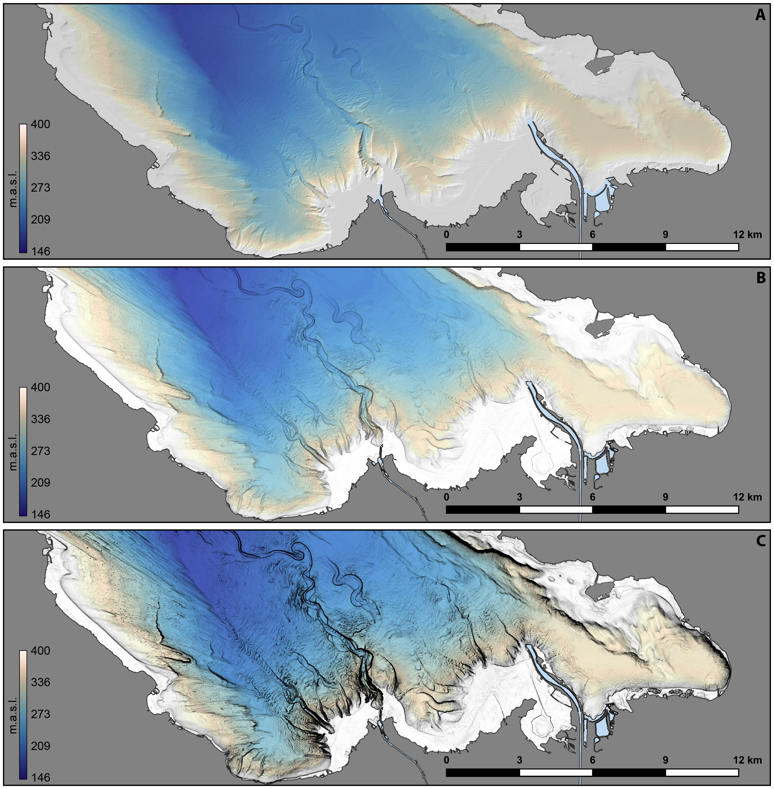
Figure 4 Examples of visualization in a predominantly high-gradient setting (dataset from LC): (A) HS A315_H40_Ve1; (B) SVF R10_D16; (C) ASVF R10_D16_An315. All three images contain a bathymetric overlay (“lapaz” colourbar from Crameri, 2018a; Crameri, 2018b; Crameri et al., 2020).

In very low-gradient settings, special attention should be given to the Ve parameter, which needs to be higher than 1 in order to adequately highlight subtle relief features (Figure 2). In the example from Figure 2, a few meters high sandwave field is barely visible at low Ve, while a subtle, less than 1 meter deep depression in the seafloor above a buried meander belt is not even recognisable (Figures 2A, C). Both morphological features become much more pronounced when a larger Ve is used (Figures 2B, D). Contrary to the commonly used HS, the HSM, PCAHS, MSRM, SVF, and ASVF reduce the effects of a unidirectional light source (mentioned in Sect. 1). Additionally, the PCAHS algorithm is very effective in highlighting both high- and low-relief features at the same time (Figure 2E). Some additional examples of effective visualizations of low-gradient settings are shown in Figures 3B, 5B, 7B, 9B, 10D, 11B.

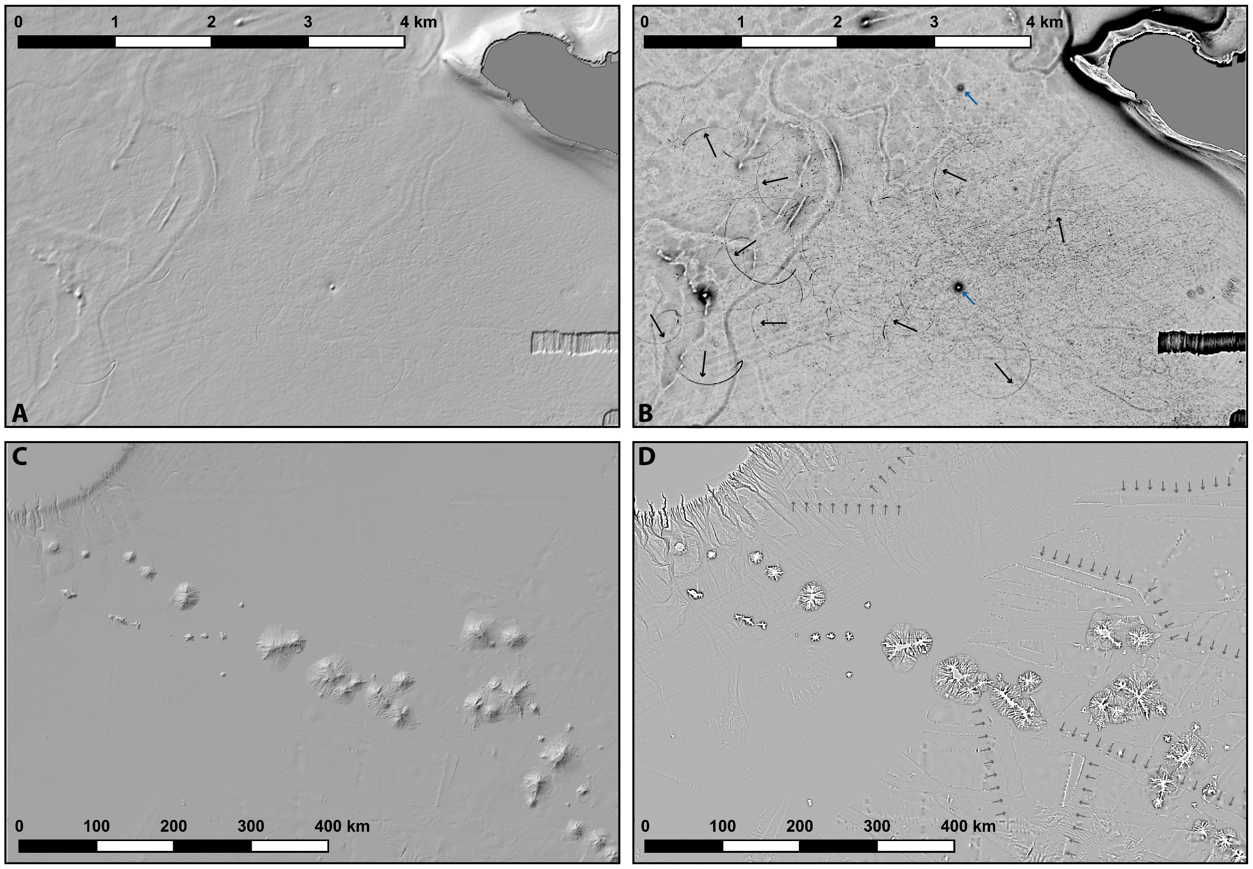
Figure 5 Visualizing narrow linear features with negligible relief (dataset: GT in A, B, NESM in C, D): (A) HS A315_H35_Ve20; (B) OPOS R10_D16 (black arrows indicate some of the more prominent bottom trawling marks (after Slavec, 2012), blue arrows indicate two archaeological features: the northerly shipwreck “barka Aura” and the southerly archaeological site “Koprske šeke” (after RKD, 2023); (C) HS A315_H40_Ve20; (D) MSRM M500-2000 (grey arrows indicate some of the more prominent artifacts at the edges of multibeam tracklines). Note how the MSRM algorithm highlights the submarine canyons in the NW corner of the inset.

In areas of both high and low topographic gradient HS is commonly used as it creates an intuitive overview of the general topographic features of the research area (e.g. Figure 3A). However, subtle topographic features can be overlooked when choosing a (too) low Ve value. Alternatively, very rugged terrain can be too dark due to setting a (too) high Ve value. In such mixed topographical settings the MSRM visualization can be a good alternative since it is very effective in highlighting escarpments in high-relief areas as well as subtle topographic features in low-relief settings. The example in Figure 3B shows well-delineated ridges, escarpments, and mass-transport deposit bodies (cf. Figure 2 from Hilbe et al., 2011 and Figure 2 from Sammartini et al., 2021). Very subtle features in low-gradient settings are also highlighted by this visualization such as the compressional ridges on the frontal bulges of the landslides. Finally, several other “mass-transport deposit-like” morphological features are visible west of WSC (Figure 3B), which could tentatively be a topographic expression of buried mass-movements (already documented in LL by Schnellmann et al., 2002; Schnellmann et al., 2006). Some additional examples of effective visualizations of both low- and high-gradient settings are shown in Figures 2E, 7B, 11B.

Relief in high-gradient settings can be quite effectively portrayed by using HS (e.g. Figure 4A), however a low Ve value should be chosen to avoid overexaggerated shadows produced by high relief. Another useful alternative is the use of the SVF and ASVF algorithms. Examples in Figures 4B, D show that these visualizations highlight more details compared to HS, while still being as intuitive as HS. Some additional examples of effective visualizations in high-gradient settings are shown in Figures 6B, 10B, 11B.

Figure 6 Visualizing convex linear and elongate features (dataset from LL): (A) HS A315_H20_Ve1; (B) SLRM R20. Black arrows indicate the ridge of the Nase moraine (after Hilbe et al., 2011; Hilbe et al., 2016). Note also how the morphological features of the gullies (indicated by white arrows), mass-movement deposits (MM; after Hilbe et al., 2011) and a fan (F; after Hilbe et al., 2011) are highlighted by the SLRM algorithm. The linearly distributed dots in the top part of both figures are acquisition artefacts.

3.2 Narrow linear features with negligible relief

Narrow linear features with negligible relief are highlighted best by the MSRM, SVF, ASVF ONEG, OPOS, and LD algorithms (Table 3). Compared to HS, these visualizations accentuate subtle features such as trawling marks and edges of multibeam tracks, which are barely visible on HS (Figure 5). While the vertical offset in case of the edges of multibeam tracks can be in the order of a few ten meters in the deep ocean setting (e.g. Figures 5C, D), the example from Figure 5B demonstrates that features can be highlighted by the appropriate algorithm even when the vertical offset amounts to less than a decimetre. Some additional examples with accentuated narrow linear features with negligible relief are included in Figures 7B, 8B, 10D.

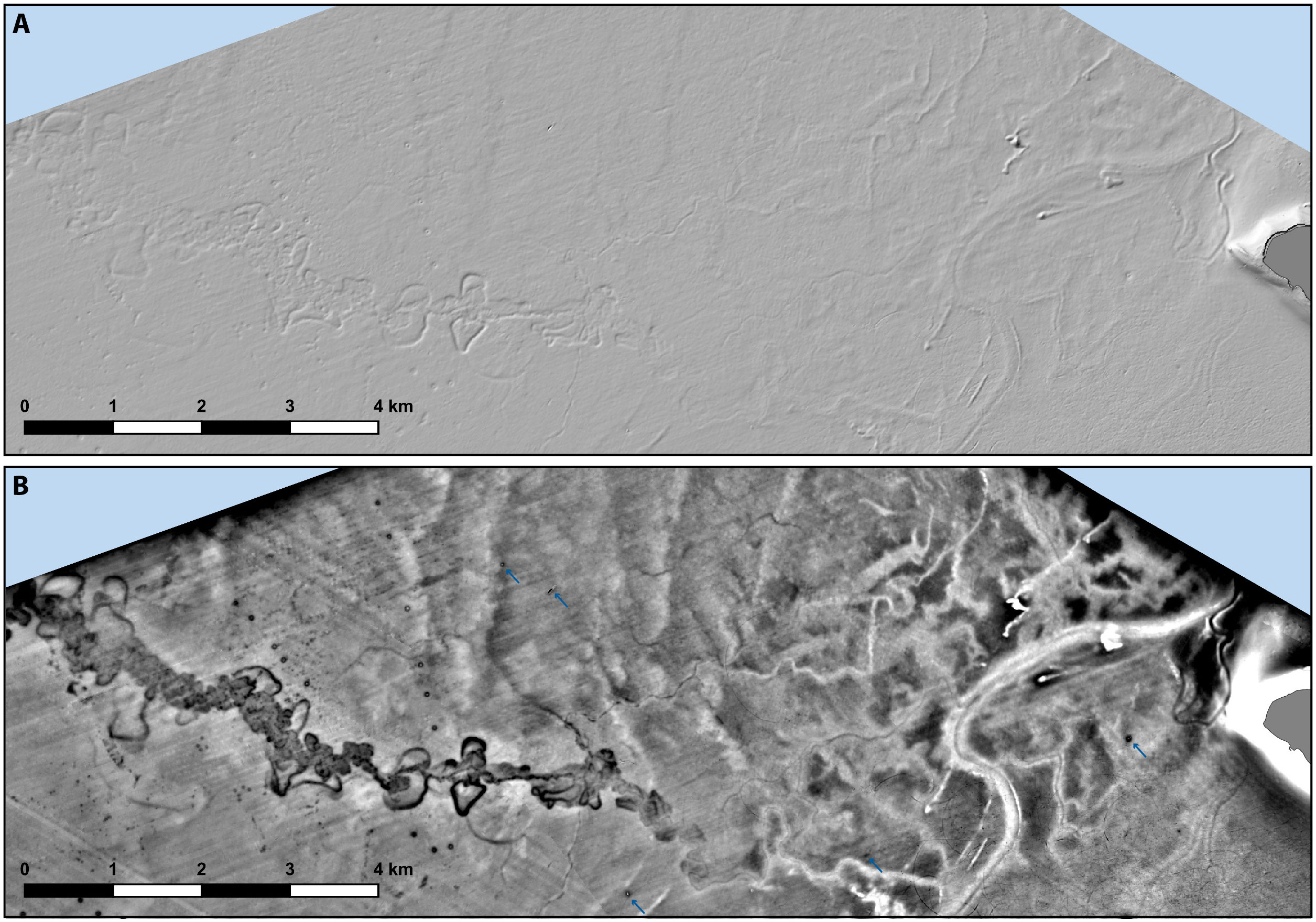
Figure 7 Visualizing concave linear and elongate features (dataset from GT): (A) HS A315_H35_Ve20; (B) LD M5_50. Note how the LD algorithm highlights the channels within the meandering belt and the related abandoned channels – relict oxbow lakes (after Trobec et al., 2017). The algorithm also highlights the sinuous fluvial channel (after Trobec et al., 2017; Novak et al., 2020) in the eastern part of the figure, where the levee is displayed in light grey and the thalweg is clearly visible as a central dark grey linear feature. Several smaller channels scattered throughout the whole extent of the displayed area are also well pronounced by the algorithm in light and dark shades of grey. Note also the archaeological features revealed on the seabed, indicated by blue arrows in (B) (locations after RKD, 2023).

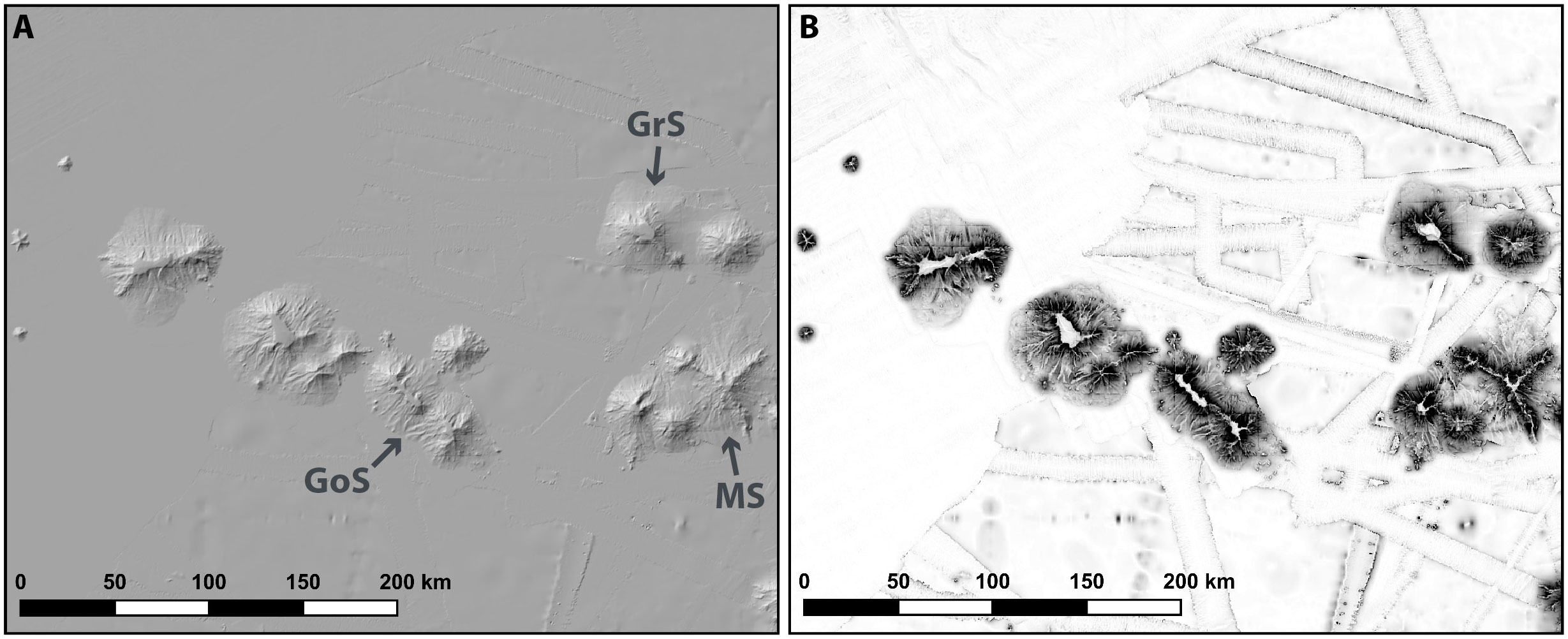
Figure 8 Visualizing linear or curved features with break in slope (dataset from NESM): (A) HS A315_H40_Ve1, (B) SVF R10 D16. Note how the SVF algorithm highlights the edges – breaks in slope of the seamounts despite of their orientation or width. Additionally, this algorithm also highlights the edges of the tracklines and the gullies and ridges along the slopes of the seamounts. GoS, GrS and MS indicate the Gosnold Seamount, Gregg Seamount and Manning Seamounts, respectively (after Flanders Marine Institute, 2022; IHO-IOC GEBCO, 2022).

3.3 Convex linear and elongate features

Convex linear and elongate features are highlighted best by the PCAHS, SLRM, MSRM, SVF, ASVF, and OPOS algorithms (Table 3). Compared to HS, these visualizations accentuate the highest parts of convex linear features regardless of their orientation. For example, the moraine ridge in Figure 6B is clearly accentuated (by brighter shades of grey) in its NE part as opposed to Figure 6A where this part of the ridge is less discernible due to its lightsource-parallel orientation. Some additional examples with accentuated convex linear and elongate features are included in Figures 2E, 3B, 5D, 7B, 9B, 10D.

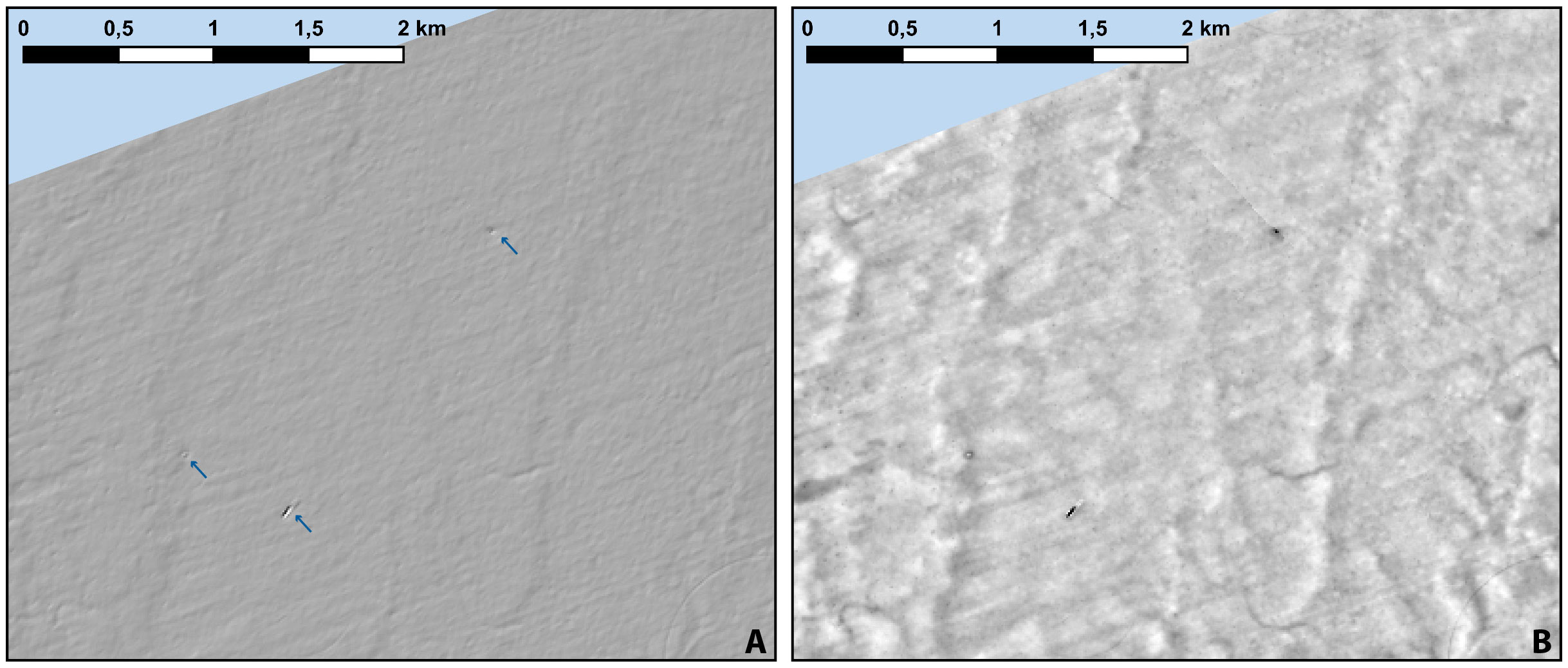
Figure 9 Visualizing circular-rounded convex features (dataset from GT): (A) HS A315_H35_Ve20; (B) SLRM R15. Note how the SLRM algorithm highlights the up to a few ten meters wide shipwrecks (indicated by blue arrows in (A) by darker shades of grey. The shipwrecks from left to right are: vessel “Barka Skale”, barge “Konji I” and vessel “Stojanov bark” (after RKD, 2023).

Figure 10 Visualizing circular-rounded concave features (dataset from LC): (A) HS A315_H40_Ve1, (B) OPOS R10_D16, (C) HS A315_H40_Ve1, and (D) OPOS R10_D16. Note how the OPOS algorithm in (B) highlights aligned pockmarks on the shoulder (indicated by black arrows) of an old channel of the Rhine (after Wessels et al., 2010). Additionally, in the central part of (B) the algorithm highlights pockmarks within an old channel filled by ripples (after Wessels et al., 2010; Bussmann et al., 2011). In (D) the algorithm was used for highlighting another area of pockmarks in LC (after Wessels et al., 2017). Note that the algorithm was used in both high- (B) and low-gradient settings (D).

3.4 Concave linear and elongate features

Convex linear and elongate features are highlighted best by the HSM, PCAHS, SLRM, MSRM, SVF, ASVF, ONEG, and LD algorithms (Table 3). Compared to HS these visualizations accentuate the deepest parts of convex linear and elongate features regardless of their depth of incision. For example, smaller channels (incised less than 0.5 m) which are barely visible when using HS (Figure 7A) are well pronounced when an appropriate algorithm is used (Figure 7B). The small channels are well accentuated even when compared to the larger and deeper fluvial channels (Figure 7B). The LD algorithm is especially suited for displaying areas containing both incised channels and channels with developed levees (i.e. with convex morphologies; Figure 7B). Some additional examples with accentuated convex linear and elongate features are included in Figures 2E, 4B, C, 5D, 6B, 9B, 10B, 11B.

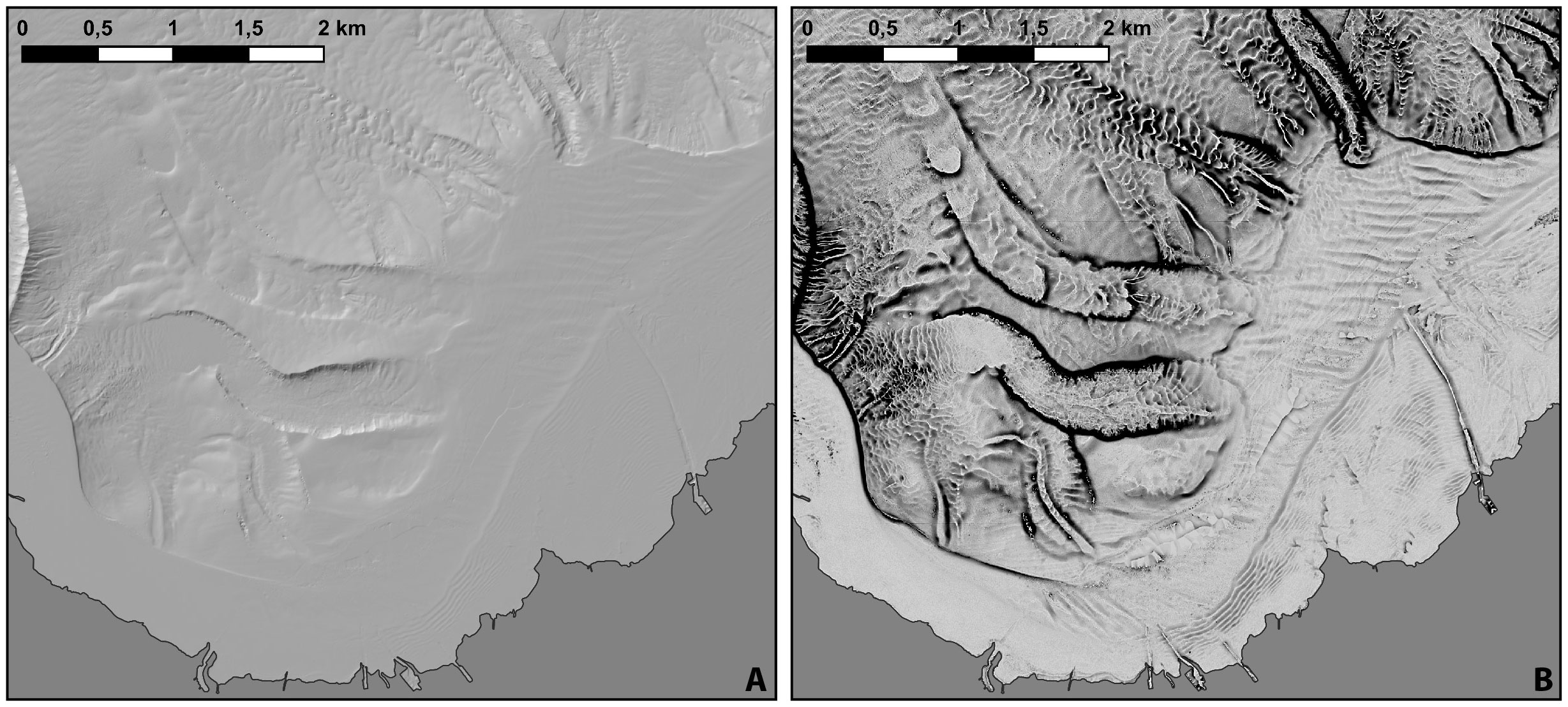
Figure 11 Visualizing features with a currogated/folded morphology (dataset from LC): (A) HS A315_H40_Ve1, (B) ONEG R10_D16. The algorithm clearly highlights bedforms in various scales: the shore-parallel megaripples (wavelengths of between 20 and 40 m; after Wessels et al., 2015), the shore-perpendicular bedforms (wavelengths between 50 and 100 m), and the bedforms between and within old channels (wavelengths between 50 and 100 m). Note that the shore-parallel and shore-perpendicular bedforms are situated in a low-gradient setting, while the other group of bedforms is located within medium- to high-gradient settings.

3.5 Linear or curved features with break in slope

Linear or curved features with break in slope are highlighted best by the HSM, PCAHS, SVF, and ASVF algorithms (Table 3). Compared to HS these algorithms highlight the break in slope much more clearly as is demonstrated in Figure 8. Additionally, these features are emphasized regardless of their orientation. For example, the edges of the NW-SE oriented seamounts (e.g. Gosnold Seamount, Gregg Seamount, eastern part of Manning Seamounts) are not very evident in Figure 8A, while they are clearly delineated in Figure 8B. Some additional examples with accentuated linear or curved features with break in slope are included in Figures 3B, 4B, C, 5D, 6B, 11B.

3.6 Circular-rounded convex features

Circular-rounded convex features are well highlighted by all the algorithms (Table 3). Compared to HS, these algorithms highlight the features regardless of how much they protrude from the sea-, lake- or riverbed as is demonstrated with the shipwrecks in Figure 9. For example, the smallest shipwreck in Figure 9 - “Barka Skale” is emphasized by the SLRM algorithm (Figure 9B) despite its relatively modest extent of 24 x 15 m (after RKD, 2023). Considering that the cell size of the used dataset is fairly large (10 x 10 m, see Table 1) this clearly demonstrates the effectiveness of the algorithm even when the features are represented by just a few pixels. Some additional examples of accentuated archaeological features are included in Figures 5B, 7B, 8B. The algorithms work well also when highlighting large-scale circular-rounded convex features, such as seamounts (e.g. Figures 5D, 8B) or outcrops and boulders (Figure 3B).

3.7 Circular-rounded concave features

Circular-rounded concave features are well highlighted by all the algorithms (Table 3). Compared to HS, these algorithms highlight the features regardless of the gradient of the studied area and the relative depth of the features compared to their surroundings (Figure 10). The example in Figure 10 demonstrates how these algorithms pronounce the pockmarks fields compared to the HS algorithm. The algorithms work well in high- (Figure 10B) as well as in low-gradient settings (Figure 10D). Some additional examples with accentuated circular-rounded concave features are included in Figures 2D, E, 4B, C, 7B, 11B.

3.8 Features with a corrugated/folded morphology

Features with a corrugated/folded morphology are highlighted best by the SLRM, MSRM, ONEG, OPOS, and LD algorithms. These algorithms pronounce the corrugated morphology which would otherwise be very subtly expressed by the HS algorithm (Figure 11). Additionally, as already demonstrated in several cases from previous sections, these algorithms highlight features regardless of their orientation. An evident example is demonstrated in the bottom central part of Figure 11B where the NE-SE oriented bedforms are much more pronounced compared to Figure 11A. As is demonstrated in Figure 11, the ONEG algorithm highlights bedforms in both low- and high-gradient settings. Some additional examples with accentuated features with a corrugated/folded morphology are included in Figures 2D, E, 3B, 4B, C, 5D, 6B, 10B, D.

4 Discussion

Visual communication of data, results and interpretation has always been a vital part of geosciences, albeit more often than not subconsciously (Libarkin and Brick, 2002; Alcalde et al., 2017; Morse et al., 2019; Crameri et al., 2020 among others). Especially in recent years with the ever-increasing amount and coverage of the Earth’s surface with high-resolution DEMs it has become even more important to strive towards effective representation and communication of elevation data. This is even more significant in the case of bathymetric data where possibilities for direct observations are severely limited compared to the onshore realm (Weatherall et al., 2015; Mayer et al., 2018; Wölfl et al., 2019). In this sense, the good and proven practices for visualization of land elevation data should be considered, transferred, and implemented also for offshore data.

The algorithms contained in RVT have been used in a variety of studies and applications demonstrated by the extensive list of more than 400 references available on their website (RVT, 2023). More than half of these are represented by archaeological studies, where RVT (and especially SVF) is commonly used for representation of elevation data (some examples include Burigana and Magnini, 2017; Masini et al., 2018; Costa-García et al., 2019; Kokalj and Somrak, 2019; Bernardini and Vinci, 2020; Lim et al., 2020; Lozić and Štular, 2021; Šprajc et al., 2022; Affek et al., 2022; Danese et al., 2022). Use of RVT is much less common in geoscientific studies which represent less than ten percent of the references (RVT, 2023). Among these, RVT is most commonly used to create visualizations in landslide research (Van Den Eeckhaut et al., 2012; Lo et al., 2017; Tsou et al., 2017; Chudý et al., 2019; Knevels et al., 2019; Verbovšek et al., 2019; Guo et al., 2021) and geomorphology (Atkinson et al., 2014; Carrasco et al., 2020; Tóth et al., 2020; Novak and Oštir, 2021; Rolland et al., 2022), while other geoscientific topics are represented by just a few papers (Mateo Lázaro et al., 2014; Djuricic et al., 2016; Favalli and Fornaciai, 2017; Delaney et al., 2018; Favalli et al., 2018; Lkebir et al., 2020; Craven et al., 2021; Delaney, 2022; Jamšek Rupnik et al., 2022). The large discrepancy between the use of RVT in archeological vs geoscientific studies indicates the unrecognised potential for alternative visualization of elevation data in geosciences. An even more striking disparity becomes evident when we consider the type of the input elevation data – to our knowledge only a few instances of the use of RVT for bathymetric data exist in published literature (Craven et al., 2021) and they are mostly limited to archaeological studies (Doneus et al., 2013; Doneus et al., 2020). This highlights the need and potential for (better) alternative visualizations of bathymetric data in geosciences, especially when we consider that the bathymetry of the research area often controls later decision regarding the locations of sampling points/coring or geophysical profiles.

Our work demonstrates that excellent results can be obtained with RVT also with bathymetric data of various resolution and from different geological and geographical settings (Section 3). All the examples shown in Figures 2–11 demonstrate that the algorithms outperform HS in every tested scenario – either when visualizing the general morphology of a study area, or when identifying specific feature shapes. One of the greatest strengths of the algorithms provided by the RVT is the possibility to highlight the feature shape of interest (Table 3). This not only facilitates the communication of observations and interpretations of digital bathymetric models, but also allows more accurate sea-, lake-, or riverbed mapping. Additionally, it has great potential to serve as an aid for locating points of interest for further surveys, not only in geoscientific, environmental, or archaeological applications, but also in search and salvage efforts (e.g. for shipwreck sites, locations of lost cargo, …). The results summarized in Table 3 indicate the most suitable algorithms for highlighting features of interest and provide a reference for future users of RVT in submerged marine, lacustrine and fluvial settings.

The quality of the visualizations produced by the algorithms of the RVT is obviously dependent on the set parameters. In this work we only demonstrate the effects of an improper setting for the Ve parameter, which results in sub-optimal visualizations (Figure 2). However, low-quality visualizations can also result from improper settings of all the other parameters which are listed at the beginning of Section 3. When deciding on the values of the parameters, RVT users should consult the RVT manual (Kokalj et al., 2019) which contains the basic guidelines for parameter determination.

While we focus on the use of the RVT software in this paper, it should be noted that several of the described algorithms are also integrated into other open and licensed software solutions, such as Global Mapper, ArcGIS, Whitebox software, QGIS, etc. with HSM being one of the most wide spread algorithms as it is presently optional in all the mentioned solutions. However, several other algorithms (e.g. ONEG, OPOS, SVF, etc.) are also available in some of the mentioned programs.

Finally, it should be pointed out that the examples demonstrated in his paper are used only for qualitatively improving the visual representation of sea-, lake-, and riverbed features and are prone to the subjective bias. For unbiased results one should revert to quantitative geomorphometric analyses, such as feature extraction and automated classification (see Lecours et al., 2016).

5 Conclusions

This work deals with the visual representation of bathymetric data by using non-standard algorithms with the intention to present a user-friendly alternative to conventional visualization techniques for displaying sea-, lake-, and riverbed morphology. We test out the algorithms on digital bathymetric models which were created from different types of bathymetric data, have different resolutions, cover the shallow-to-abbysal depth range and span through different regions and settings. We identify the best algorithms to display the general morphology of a study area and the optimal algorithms for highlighting geomorphic features of interest. The results of our tests show that the algorithms contained within RVT are far superior to the conventional Hillshade and Slope gradient visualization techniques for bathymetric data. We provide a summary of our observations which can be considered a promotion of the RVT within the offshore and submerged terrestrial scientific community and as a set of guidelines for future users of RVT working in the offshore and submerged terrestrial domains. Our study demonstrates the importance, versatility, and efficacy of RVT for the creation of better and more informative bathymetric data visualizations.

Data availability statement

Publicly available datasets were analyzed in this study. This data can be found here: https://www.swisstopo.admin.ch/en/geodata/height/bathy3d.html, https://doi.org/10/gn6h.

Author contributions

AN: Conceptualization, Data curation, Formal Analysis, Funding acquisition, Investigation, Methodology, Validation, Visualization, Writing – original draft, Writing – review & editing. SP: Data curation, Investigation, Writing – review & editing. MV: Funding acquisition, Writing – review & editing.

Funding

The author(s) declare financial support was received for the research, authorship, and/or publication of this article. This study was supported by the Slovenian Research and Innovation Agency (ARIS) [research programmes P1-0011 & P1-0195; research projects J1-1712 & L1-5452 (co-funded by Harpha Sea d.o.o.)]; and the Slovenian National Commission for UNESCO, International Geoscience Programme [projects IGCP 639 and 725].

Acknowledgments

This study benefited from the discussions at several meetings of the NEPTUNE project (New Procedures and Technologies for Underwater Paleo-landscape Reconstruction) funded as project nr. 2003P by the International Union for Quaternary Research (INQUA). Finally, we would like thank Luis A. Conti, Vincent Lecours, and reviewer for their valuable comments.

Conflict of interest

Author SP is employed by Sirio d.o.o, Slovenia.

The remaining authors declare that the research was conducted in the absence of any commercial or financial relationships that could be construed as a potential conflict of interest.

Publisher’s note

All claims expressed in this article are solely those of the authors and do not necessarily represent those of their affiliated organizations, or those of the publisher, the editors and the reviewers. Any product that may be evaluated in this article, or claim that may be made by its manufacturer, is not guaranteed or endorsed by the publisher.

References

Affek A. N., Wolski J., Latocha A., Zachwatowicz M., Wieczorek M. (2022). The use of LiDAR in reconstructing the pre-World War II landscapes of abandoned mountain villages in southern Poland. Archaeol. Prospect. 29, 157–173. doi: 10.1002/arp.1846
Aiello G., Sacchi M. (2022). New morpho-bathymetric data on marine hazard in the offshore of Gulf of Naples (Southern Italy). Nat. Hazards 111, 2881–2908. doi: 10.1007/s11069-021-05161-2
Alcalde J., Bond C. E., Randle C. H. (2017). Framing bias: The effect of figure presentation on seismic interpretation. Interpretation 5, T591–T605. doi: 10.1190/INT-2017-0083.1
Atkinson N., Utting D. J., Pawley S. M. (2014). Landform signature of the Laurentide and Cordilleran ice sheets across Alberta during the last glaciation. Can. J. Earth Sci. 51, 1067–1083. doi: 10.1139/cjes-2014-0112
Bernardini F., Vinci G. (2020). Archaeological landscape in central northern Istria (Croatia) revealed by airborne LiDAR: from prehistoric sites to Roman centuriation. Archaeol. Anthropol. Sci. 12, 133. doi: 10.1007/s12520-020-01070-w
Berthod C., Bachèlery P., Jorry S. J., Pitel-Roudaut M., Ruffet G., Revillon S., et al. (2022). First characterization of the volcanism in the southern Mozambique Channel: Geomorphological and structural analyses. Mar. Geol. 445, 106755. doi: 10.1016/j.margeo.2022.106755
Burigana L., Magnini L. (2017). Image processing and analysis of radar and lidar data: new discoveries in Verona southern lowland (Italy). STAR: Sci. Technol. Archaeol. Res. 3, 490–509. doi: 10.1080/20548923.2018.1426273
Busetti M., Volpi V., Barison E., Giustiniani M., Marchi M., Ramella R., et al. (2010a). Meso-Cenozoic seismic stratigraphy and the tectonic setting of the Gulf of Trieste (northern Adriatic). GeoActa SP 3, 1–14.
Busetti M., Volpi V., Nicolich R., Barison E., Romeo R., Baradello L., et al. (2010b). Dinaric tectonic features in the Gulf of Trieste (Northern Adriatic Sea). Bollettino di Geofisica Teorica ed Applicata 51, 117–128.
Bussmann I., Schlömer S., Schlüter M., Wessels M. (2011). Active pockmarks in a large lake (Lake Constance, Germany): Effects on methane distribution and turnover in the sediment. Limnol. Oceanogr. 56, 379–393. doi: 10.4319/LO.2011.56.1.0379
Caporizzo C., Aucelli P. P. C., Di Martino G., Mattei G., Tonielli R., Pappone G. (2021). Geomorphometric analysis of the natural and anthropogenic seascape of Naples (Italy): A high-resolution morpho-bathymetric survey. Trans. GIS 25, 2571–2595. doi: 10.1111/tgis.12829
Carrasco R. M., Soteres R. L., Pedraza J., Fernández-Lozano J., Turu V., Antonio López-Sáez J., et al. (2020). Glacial geomorphology of the High Gredos Massif: Gredos and Pinar valleys (Iberian Central System, Spain). J. Maps 16, 790–804. doi: 10.1080/17445647.2020.1833768
Chudý F., Slámová M., Tomaštík J., Prokešová R., Mokroš M. (2019). Identification of micro-scale landforms of landslides using precise digital elevation models. Geosciences 9, 117. doi: 10.3390/geosciences9030117
Costa-García J.-M., Fonte J., Gago M. (2019). The reassessment of the Roman military presence in Galicia and northern Portugal through digital tools: archaeological diversity and historical problems. Mediterr. Archaeol. Archaeometry 19, 17–49. doi: 10.5281/zenodo.3457524
Crameri F. (2018a). Geodynamic diagnostics, scientific visualisation and StagLab 3.0. Geosci. Model. Dev. 11, 2541–2562. doi: 10.5194/gmd-11-2541-2018
Crameri F., Shephard G. E., Heron P. J. (2020). The misuse of colour in science communication. Nat. Commun. 11, 5444–5444. doi: 10.1038/s41467-020-19160-7
Craven K. F., McCarron S., Monteys X., Dove D. (2021). Interaction of multiple ice streams on the Malin Shelf during deglaciation of the last British–Irish Ice Sheet. J. Quaternary Sci. 36, 153–168. doi: 10.1002/jqs.3266
Danese M., Gioia D., Vitale V., Abate N., Amodio A. M., Lasaponara R., et al. (2022). Pattern recognition approach and liDAR for the analysis and mapping of archaeological looting: application to an etruscan site. Remote Sens. 14, 1587. doi: 10.3390/rs14071587
Delaney C. (2022). The development and impact of an ice-contact proglacial lake during the Last Glacial Termination, Palaeolake Riada, central Ireland. J. Quaternary Sci. 37, 1422–1441. doi: 10.1002/jqs.3412
Delaney C. A., McCarron S., Davis S. (2018). Irish Ice Sheet dynamics during deglaciation of the central Irish Midlands: Evidence of ice streaming and surging from airborne LiDAR. Geomorphology 306, 235–253. doi: 10.1016/j.geomorph.2018.01.011
De Reu J., Bourgeois J., Bats M., Zwertvaegher A., Gelorini V., De Smedt P., et al. (2013). Application of the topographic position index to heterogeneous landscapes. Geomorphology 186, 39–49. doi: 10.1016/j.geomorph.2012.12.015
Djuricic A., Dorninger P., Nothegger C., Harzhauser M., Székely B., Rasztovits S., et al. (2016). High-resolution 3D surface modeling of a fossil oyster reef. Geosphere 12, 1457–1477. doi: 10.1130/GES01282.1
Doneus M., Doneus N., Briese C., Pregesbauer M., Mandlburger G., Verhoeven G. (2013). Airborne laser bathymetry – detecting and recording submerged archaeological sites from the air. J. Archaeol. Sci. 40, 2136–2151. doi: 10.1016/J.JAS.2012.12.021
Doneus N., Miholjek I., Džin K., Doneus M., Dugonjić P., Schiel H. (2020). Archaeological prospection of coastal and submerged settlement sites. Re-evaluation of the roman site complex of Vižula, Croatia. Archaeol. Austriaca 104/2, 235–281. doi: 10.1553/archaeologia104s235
Drăguţ L., Eisank C. (2011). Object representations at multiple scales from digital elevation models. Geomorphology 129, 183–189. doi: 10.1016/j.geomorph.2011.03.003
Duncan R. A. (1984). Age progressive volcanism in the New England Seamounts and the opening of the central Atlantic Ocean. J. Geophys. Res.: Solid Earth 89, 9980–9990. doi: 10.1029/JB089iB12p09980
EuroGeographics, UN-FAO (2020) Data from: Countries 2020 - Administrative Units – Dataset. Available at: https://ec.europa.eu/eurostat/web/gisco/geodata/reference-data/administrative-units-statistical-units/countries (Accessed 1.4.2022).
Fabbri S. C., Haas I., Kremer K., Motta D., Girardclos S., Anselmetti F. S. (2021). Subaqueous geomorphology and delta dynamics of Lake Brienz (Switzerland): implications for the sediment budget in the alpine realm. Swiss J. Geoscie. 114, 22. doi: 10.1186/s00015-021-00399-1
Favalli M., Fornaciai A. (2017). Visualization and comparison of DEM-derived parameters. Application to volcanic areas. Geomorphology 290, 69–84. doi: 10.1016/j.geomorph.2017.02.029
Favalli M., Fornaciai A., Nannipieri L., Harris A., Calvari S., Lormand C. (2018). UAV-based remote sensing surveys of lava flow fields: a case study from Etna’s 1974 channel-fed lava flows. Bull. Volcanol 80, 29. doi: 10.1007/s00445-018-1192-6
Federal Office of Topography swisstopo (2021) Data from: swissBATHY3D. Available at: https://www.swisstopo.admin.ch/en/geodata/height/bathy3d.html (Accessed 1.4.2022).
Flanders Marine Institute (2018) Data from: IHO Sea Areas, version 3. doi: 10.14284/323 (Accessed 1.3.2022).
Flanders Marine Institute (2022) Marine Regions Gazetteer. Available at: https://marineregions.org/gazetteer.php?p=search (Accessed 15.6.2022).
GEBCO (2021) The GEBCO_2021 Grid (NERC EDS British Oceanographic Data Centre NOC). Available at: https://www.gebco.net/data_and_products/gridded_bathymetry_data/gebco_2021/ (Accessed 30.3.2022).
GEBCO Group (2021) Data from: The GEBCO_2021 Grid - a continuous terrain model of the global oceans and land (NERC EDS British Oceanographic Data Centre NOC). (Accessed 15.3.2022).
Georgiou N., Dimas X., Fakiris E., Christodoulou D., Geraga M., Koutsoumpa D., et al. (2021). A multidisciplinary approach for the mapping, automatic detection and morphometric analysis of ancient submerged coastal installations: the case study of the ancient aegina harbour complex. Remote Sens. 13, 4462. doi: 10.3390/rs13214462
Guisan A., Weiss S. B., Weiss A. D. (1999). GLM versus CCA spatial modeling of plant species distribution. Plant Ecol. 143, 107–122. doi: 10.1023/A:1009841519580
Guo C., Xu Q., Dong X., Li W., Zhao K., Lu H., et al. (2021). Geohazard recognition and inventory mapping using airborne liDAR data in complex mountainous areas. J. Earth Sci. 32, 1079–1091. doi: 10.1007/s12583-021-1467-2
Heaman L. M., Kjarsgaard B. A. (2000). Timing of eastern North American kimberlite magmatism: continental extension of the Great Meteor hotspot track? Earth Planet. Sci. Lett. 178, 253–268. doi: 10.1016/S0012-821X(00)00079-0
Hilbe M., Anselmetti F. S., Eilertsen R. S., Hansen L., Wildi W. (2011). Subaqueous morphology of Lake Lucerne (Central Switzerland): implications for mass movements and glacial history. Swiss J. Geoscie. 104, 3 104, 425–443. doi: 10.1007/S00015-011-0083-Z
Hilbe M., Strupler M., Hansen L., Eilertsen R. S., Daele M. V., Batist M. D., et al. (2016). Moraine ridges in fjord-type, perialpine Lake Lucerne, central Switzerland. Geol. Society London Memoirs 46, 69–70. doi: 10.1144/M46.107
Hughes Clarke J. E. (2018). “Multibeam Echosounders,” in Submarine Geomorphology Springer Geology. Eds. Micallef A., Krastel S., Savini A. (Cham: Springer International Publishing), 25–41. doi: 10.1007/978-3-319-57852-1_3
Hupy J. P., Schaetzl R. J. (2006). Introducing “bombturbation,” a singular type of soil disturbance and mixing. Soil Sci. 171, 823–836. doi: 10.1097/01.ss.0000228053.08087.19
IHO-IOC GEBCO (2022) IHO-IOC GEBCO Gazetteer of Undersea Feature Names, version 4.3.6 – web map application. Available at: https://www.ngdc.noaa.gov/gazetteer/ (Accessed 14.6.2022).
Jamšek Rupnik P., Žebre M., Jež J., Zajc M., Preusser F., Monegato G. (2022). Deciphering the deformation mechanism in Quaternary deposits along the Idrija Fault in the formerly glaciated Soča Valley, southeast European Alps. Eng. Geol. 297, 106515. doi: 10.1016/j.enggeo.2021.106515
Knevels R., Petschko H., Leopold P., Brenning A. (2019). Geographic object-based image analysis for automated landslide detection using open source GIS software. ISPRS Int. J. Geo-Inform. 8, 551. doi: 10.3390/ijgi8120551
Kokalj Ž., Somrak M. (2019). Why not a single image? Combining visualizations to facilitate fieldwork and on-screen mapping. Remote Sens. 11, 747–747. doi: 10.3390/rs11070747
Kokalj Ž., Zakšek K., Oštir K. (2011). Application of sky-view factor for the visualisation of historic landscape features in lidar-derived relief models. Antiquity 85, 263–273. doi: 10.1017/S0003598X00067594
Kokalj Ž., Zakšek K., Oštir K., Pehani P., Čotar K., Somrak M. (2019). Relief Visualization Toolbox, ver. 2.2.1 Manual (Ljubljana: Research Centre of the Slovenian Academy of Sciences and Arts (ZRC SAZU). Available at: https://www.zrc-sazu.si/sites/default/files/rvt_2.2.1_0.pdf.
Lebrec U., Riera R., Paumard V., O’Leary M. J., Lang S. C. (2022). Morphology and distribution of submerged palaeoshorelines: Insights from the North West Shelf of Australia. Earth-Science Rev. 224, 103864. doi: 10.1016/j.earscirev.2021.103864
Lecours V., Dolan M. F. J., Micallef A., Lucieer V. L. (2016). A review of marine geomorphometry, the quantitative study of the seafloor. Hydrol. Earth Sys. Sci. 20, 3207–3244. doi: 10.5194/hess-20-3207-2016
Li S., Alves T. M., Li W., Wang X., Rebesco M., Li J., et al. (2022). Morphology and evolution of submarine canyons on the northwest South China Sea margin. Mar. Geol. 443, 106695. doi: 10.1016/j.margeo.2021.106695
Libarkin J. C., Brick C. (2002). Research methodologies in science education: visualization and the geosciences. J. Geosci. Educ. 50, 449–455. doi: 10.5408/1089-9995-50.4.449
Lim J., Clark J., Linares-Matás G. (2020). Subsurface delineation of doline features associated with Pleistocene clay-with-flints deposits in the Chilterns: Implications for British Palaeolithic archaeology. J. Archaeol. Science: Rep. 34, 102665. doi: 10.1016/j.jasrep.2020.102665
Lkebir N., Rolland T., Monna F., Masrour M., Bouchaou L., Fara E., et al. (2020). Anza palaeoichnological site, Late Cretaceous, Morocco. Part III: Comparison between traditional and photogrammetric records. J. Afr. Earth Sci. 172, 103985. doi: 10.1016/j.jafrearsci.2020.103985
Lo C.-M., Lee C.-F., Keck J. (2017). Application of sky view factor technique to the interpretation and reactivation assessment of landslide activity. Environ. Earth Sci. 76, 375. doi: 10.1007/s12665-017-6705-7
Lozić E., Štular B. (2021). Documentation of archaeology-specific workflow for airborne liDAR data processing. Geosciences 11, 26. doi: 10.3390/geosciences11010026
Madricardo F., Foglini F., Campiani E., Grande V., Catenacci E., Petrizzo A., et al. (2019). Assessing the human footprint on the sea-floor of coastal systems: the case of the Venice Lagoon, Italy. Sci. Rep. 9, 6615–6615. doi: 10.1038/s41598-019-43027-7
Majcher J., Plets R., Quinn R. (2020). Residual relief modelling: digital elevation enhancement for shipwreck site characterisation. Archaeol. Anthropol. Sci. 12, 122–122. doi: 10.1007/s12520-020-01082-6
Manstretta G. M. M., Arena M., Perillo G. M. E., Vitale A. J., Payares Peña N. B., Ferronato C., et al. (2022). Sediment bank contribution to form a vortex and maintain a deep scour hole on tidal channel meander in the Bahía Blanca estuary, Argentina. J. South Am. Earth Sci. 115, 103745. doi: 10.1016/j.jsames.2022.103745
Marple R. T., Hurd J. D. (2019). Sonar and LiDAR investigation of lineaments offshore between central New England and the New England seamounts, USA. Atlantic Geol. 55, 57–91. doi: 10.4138/atlgeol.2019.002
Marple R. T., James D. Hurd J., Altamura R. J. (2018). Ring-shaped morphological features and interpreted small seamounts between southern Quebec (Canada) and the New England seamounts (USA) and their possible association with the New England hotspot track. Atlantic Geol. 54, 223–265. doi: 10.4138/atlgeol.2018.008
Masini N., Gizzi F. T., Biscione M., Fundone V., Sedile M., Sileo M., et al. (2018). Medieval archaeology under the canopy with liDAR. The (Re)Discovery of a medieval fortified settlement in southern Italy. Remote Sens. 10, 1598. doi: 10.3390/rs10101598
Mateo Lázaro J., Sánchez Navarro J.Á., García Gil A., Edo Romero V. (2014). 3D-geological structures with digital elevation models using GPU programming. Comput. Geoscie. 70, 138–146. doi: 10.1016/j.cageo.2014.05.014
Maxwell A. E., Shobe C. M. (2022). Land-surface parameters for spatial predictive mapping and modeling. Earth-Science Rev. 226, 103944. doi: 10.1016/j.earscirev.2022.103944
Mayer L., Jakobsson M., Allen G., Dorschel B., Falconer R., Ferrini V., et al. (2018). The nippon foundation—GEBCO seabed 2030 project: the quest to see the world’s oceans completely mapped by 2030. Geosciences 8, 63. doi: 10.3390/geosciences8020063
Merle R. E., Jourdan F., Chiaradia M., Olierook H. K. H., Manatschal G. (2019). Origin of widespread Cretaceous alkaline magmatism in the Central Atlantic: A single melting anomaly? Lithos 342–343, 480–498. doi: 10.1016/j.lithos.2019.06.002
Micallef A., Krastel S., Savini A. (2018). “Introduction,” in Submarine Geomorphology Springer Geology. Eds. Micallef A., Krastel S., Savini A. (Cham: Springer International Publishing), 1–9. doi: 10.1007/978-3-319-57852-1_1
Morse P. E., Reading A. M., Stål T. (2019). Well-posed geoscientific visualization through interactive color mapping. Front. Earth Sci. 7. doi: 10.3389/feart.2019.00274
Müller G., Gees R. A. (1968). Origin of the lake constance basin. Nature 217, 836–837. doi: 10.1038/217836a0
Novak A., Oštir K. (2021). Towards better visualisation of alpine quaternary landform features on high-resolution digital elevation models. Remote Sens. 13, 4211. doi: 10.3390/rs13214211
Novak A., Šmuc A., Poglajen S., Vrabec M. (2020). Linking the high-resolution acoustic and sedimentary facies of a transgressed Late Quaternary alluvial plain (Gulf of Trieste, northern Adriatic). Mar. Geol. 419, 106061. doi: 10.1016/j.margeo.2019.106061
Ogorelec B., Mišič M., Faganeli J. (1991). Marine geology of the Gulf of Trieste (northern Adriatic): Sedimentological aspects. Mar. Geol. 99, 79–92. doi: 10.1016/0025-3227(91)90084-H
Onorati G., Ventura R., Poscolieri M., Chiarini V., Crucillà U. (1992). The Digital Elevation Model of Italy for geomorphology and structural geology. Catena 19, 147–178. doi: 10.1016/0341-8162(92)90022-4
Orengo H. A., Petrie C. A. (2018). Multi-scale relief model (MSRM): a new algorithm for the visualization of subtle topographic change of variable size in digital elevation models. Earth Surf. Processes Landforms 43, 1361–1369. doi: 10.1002/esp.4317
Piret L., Bertrand S., Nguyen N., Hawkings J., Rodrigo C., Wadham J. (2022). Long-lasting impacts of a 20th century glacial lake outburst flood on a Patagonian fjord-river system (Pascua River). Geomorphology 399, 108080. doi: 10.1016/j.geomorph.2021.108080
Post A. L., Przeslawski R., Nanson R., Siwabessy J., Smith D., Kirkendale L. A., et al. (2022). Modern dynamics, morphology and habitats of slope-confined canyons on the northwest Australian margin. Mar. Geol. 443, 106694. doi: 10.1016/j.margeo.2021.106694
Puga-Bernabéu Á., López-Cabrera J., Webster J. M., Beaman R. J. (2022). Submarine landslide morphometrics and slope failure dynamics along a mixed carbonate-siliciclastic margin, north-eastern Australia. Geomorphology 403, 108179. doi: 10.1016/j.geomorph.2022.108179
Riddick N. L., Boyce J. I., Krezoski G. M., Şahoğlu V., Erkanal H., Tuğcu İ., et al. (2022). Palaeoshoreline reconstruction and underwater archaeological potential of Liman Tepe: A long-occupied coastal prehistoric settlement in western Anatolia, Turkey. Quaternary Sci. Rev. 276, 107293. doi: 10.1016/j.quascirev.2021.107293
RKD (2023) Registry of cultural heritage – web viewer (Ministry of Culture of the Republic of Slovenia). Available at: https://gisportal.gov.si/rkd (Accessed 20.7.2023).
Rolland T., Monna F., Buoncristiani J. F., Magail J., Esin Y., Bohard B., et al. (2022). Volumetric obscurance as a new tool to better visualize relief from digital elevation models. Remote Sens. 14, 941. doi: 10.3390/rs14040941
Ronchi L., Fontana A., Novak A., Correggiari A., Poglajen S. (2023). Late-quaternary evolution of the semi-confined alluvial megafan of Isonzo river (Northern Adriatic): where the fluvial system of the southern alps meets the karst. Geosciences 13 (5), 135. doi: 10.3390/geosciences13050135
RVT (2023) Relief Visualization Toolbox in Python documentation (ZRC SAZU and University of Ljubljana). Available at: https://rvt-py.readthedocs.io/ (Accessed 15.9.2023).
Sammartini M., Moernaut J., Kopf A., Stegmann S., Fabbri S. C., Anselmetti F. S., et al. (2021). Propagation of frontally confined subaqueous landslides: Insights from combining geophysical, sedimentological, and geotechnical analysis. Sedimentary Geol. 416, 105877–105877. doi: 10.1016/J.SEDGEO.2021.105877
Sandwell D. T., Goff J. A., Gevorgian J., Harper H., Kim S.-S., Yu Y., et al. (2022). Improved bathymetric prediction using geological information: SYNBATH. Earth Space Sci. 9, e2021EA002069. doi: 10.1029/2021EA002069
Schnellmann M., Anselmetti F. S., Giardini D., McKenzie J. A. (2005). Mass movement-induced fold-and-thrust belt structures in unconsolidated sediments in Lake Lucerne (Switzerland). Sedimentology 52, 271–289. doi: 10.1111/J.1365-3091.2004.00694.X
Schnellmann M., Anselmetti F. S., Giardini D., Mckenzie J. A. (2006). 15,000 Years of mass-movement history in Lake Lucerne: Implications for seismic and tsunami hazards. Eclogae Geol. Helvetiae 99, 409–428. doi: 10.1007/S00015-006-1196-7
Schnellmann M., Anselmetti F. S., Giardini D., McKenzie J. A., Ward S. N. (2002). Prehistoric earthquake history revealed by lacustrine slump deposits. Geology 30, 1131–1131. doi: 10.1130/0091-7613(2002)030<1131:PEHRBL>2.0.CO;2
Schröder H. G., Wessels M., Niessen F. (1998). Acoustic facies and depositional structures of Lake Constance. Arch. Hydrobiol. Spec. Issues Advanc. Limnol. 53, 351–368.
Slavec P. (2012). Analiza morfologije morskega dna slovenskega morja [MSc thesis]. (Ljubljana, Slovenia: University of Ljubljana)
Smith M. J., Clark C. D. (2005). Methods for the visualization of digital elevation models for landform mapping. Earth Surf. Processes Landforms 30, 885–900. doi: 10.1002/ESP.1210
Sofia G. (2020). Combining geomorphometry, feature extraction techniques and Earth-surface processes research: The way forward. Geomorphology 355, 107055. doi: 10.1016/j.geomorph.2020.107055
Šprajc I., Marsetič A., Štajdohar J., Góngora S. D., Ball J. W., Olguín O. E., et al. (2022). Archaeological landscape, settlement dynamics, and sociopolitical organization in the Chactún area of the central Maya Lowlands. PloS One 17, e0262921. doi: 10.1371/journal.pone.0262921
Strasser M., Hilbe M., Anselmetti F. S. (2010). Mapping basin-wide subaquatic slope failure susceptibility as a tool to assess regional seismic and tsunami hazards. Mar. Geophys. Res. 32, 331–347. doi: 10.1007/S11001-010-9100-2
Strasser M., Stegmann S., Bussmann F., Anselmetti F. S., Rick B., Kopf A. (2007). Quantifying subaqueous slope stability during seismic shaking: Lake Lucerne as model for ocean margins. Mar. Geol. 240, 77–97. doi: 10.1016/J.MARGEO.2007.02.016
Streuff K. T., Cofaigh C. Ó, Wintersteller P. (2022). GlaciDat – a GIS database of submarine glacial landforms and sediments in the Arctic. Boreas 51, 517–531. doi: 10.1111/bor.12577
Tarolli P. (2014). High-resolution topography for understanding Earth surface processes: Opportunities and challenges. Geomorphology 216, 295–312. doi: 10.1016/j.geomorph.2014.03.008
Telling J., Lyda A., Hartzell P., Glennie C. (2017). Review of Earth science research using terrestrial laser scanning. Earth-Science Rev. 169, 35–68. doi: 10.1016/j.earscirev.2017.04.007
Tóth Z., McCarron S., Wheeler A. J., Wenau S., Davis S., Lim A., et al. (2020). Geomorphological and seismostratigraphic evidence for multidirectional polyphase glaciation of the northern Celtic Sea. J. Quaternary Sci. 35, 465–478. doi: 10.1002/jqs.3189
Trincardi F., Argnani A., Correggiari A., Foglini F., Rovere M., Angeletti L., et al. (2011a). Note illustrative della Carta Geologica dei mari italiani alla scala 1:250.000 foglio NL 33-7 Venezia. (Ancona, Italy: Instituto di Scienze Marine, Consiglio Nazionale delle Ricerche), 151.
Trincardi F., Correggiari A., Cattaneo A., Remia A., Taviani M., Angeletti L., et al. (2011b). Carta Geologica dei mari italiani alla scala 1:250.000 foglio NL 33-7 Venezia. (Ancona, Italy: Istituto di Scienze Marine, Consiglio Nazionale delle Ricerche)
Trobec A., Busetti M., Zgur F., Baradello L., Babich A., Cova A., et al. (2018). Thickness of marine Holocene sediment in the Gulf of Trieste (northern Adriatic Sea). Earth Sys. Sci. Data 10, 1077–1092. doi: 10.5194/essd-10-1077-2018
Trobec A., Šmuc A., Poglajen S., Vrabec M. (2017). Submerged and buried Pleistocene river channels in the Gulf of Trieste (Northern Adriatic Sea): Geomorphic, stratigraphic and tectonic inferences. Geomorphology 286, 110–120. doi: 10.1016/j.geomorph.2017.03.012
Tsou C.-Y., Chigira M., Matsushi Y., Hiraishi N., Arai N. (2017). Coupling fluvial processes and landslide distribution toward geomorphological hazard assessment: a case study in a transient landscape in Japan. Landslides 14, 1901–1914. doi: 10.1007/s10346-017-0838-3
Van Den Eeckhaut M., Kerle N., Poesen J., Hervás J. (2012). Object-oriented identification of forested landslides with derivatives of single pulse LiDAR data. Geomorphology 173–174, 30–42. doi: 10.1016/j.geomorph.2012.05.024
Verbovšek T., Popit T., Kokalj Ž. (2019). VAT method for visualization of mass movement features: an alternative to hillshaded DEM. Remote Sens. 11, 2946–2946. doi: 10.3390/RS11242946
Verweirder L., Van Rooij D., White M., Van Landeghem K., Bossée K., Georgiopoulou A. (2021). Combined control of bottom and turbidity currents on the origin and evolution of channel systems, examples from the Porcupine Seabight. Mar. Geol. 442, 106639. doi: 10.1016/j.margeo.2021.106639
Walbridge S., Slocum N., Pobuda M., Wright D. J. (2018). Unified geomorphological analysis workflows with benthic terrain modeler. Geosciences 8, 94–94. doi: 10.3390/GEOSCIENCES8030094
Watson S. J., Neil H., Ribó M., Lamarche G., Strachan L. J., MacKay K., et al. (2020). What we do in the shallows: natural and anthropogenic seafloor geomorphologies in a drowned river valley, New Zealand. Front. Mar. Sci. 7. doi: 10.3389/fmars.2020.579626
Weatherall P., Marks K. M., Jakobsson M., Schmitt T., Tani S., Arndt J. E., et al. (2015). A new digital bathymetric model of the world’s oceans. Earth Space Sci. 2, 331–345. doi: 10.1002/2015EA000107
Werner F., Unsöld G., Koopmann B., Stefanon A. (1980). Field observations and flume experiments on the nature of comet marks. Sedimentary Geol. 26, 233–262. doi: 10.1016/0037-0738(80)90013-5
Wessels M., Anselmetti F., Artuso R., Baran R., Daut G., Gaide S., et al. (2015). Bathymetry of lake constance – a high-resolution survey in a large, deep lake. ZfV - Z. für Geodäsie Geoinform. und Landmanage. 140, 203–210. doi: 10.12902/ZFV-0079-2015
Wessels M., Brückner N., Gaide S., Wintersteller P. (2017). Tiefenschärfe — die hochauflösende Vermessung des Bodensees. WasserWirtschaft 107, 30–35. doi: 10.1007/S35147-017-0028-1
Wessels M., Bussmann I., Schloemer S., Schlü ter M., Bö dere V. (2010). Distribution, morphology, and formation of pockmarks in Lake Constance, Germany. Limnol. Oceanogr. 55, 2623–2633. doi: 10.4319/LO.2010.55.6.2623
Wölfl A.-C., Snaith H., Amirebrahimi S., Devey C. W., Dorschel B., Ferrini V., et al. (2019). Seafloor mapping – the challenge of a truly global ocean bathymetry. Front. Mar. Sci. 6. doi: 10.3389/fmars.2019.00283
Wu H., Zhang H., Zhang X., Peng W., Liu Q., Liu F., et al. (2021). Potential catastrophic water outflow from Lake Dian, China: Possible hydrological and ecological risks. CATENA 207, 105589. doi: 10.1016/j.catena.2021.105589
Yokoyama R., Shlrasawa M., Pike R. J. (2002). Visualizing topography by openness: A new application of image processing to digital elevation models. Photogrammetric Eng. Remote Sens. 68, 257–265.
Zakšek K., Oštir K., Kokalj Ž. (2011). Sky-view factor as a relief visualization technique. Remote Sens. 3, 398–415. doi: 10.3390/rs3020398
Zheng S., Hu H., Xu S., Cheng H., Li Z., Liu E. (2022). Spatial distribution and response of dunes to anthropogenic factors in the lower Yangtze River. CATENA 212, 106045. doi: 10.1016/j.catena.2022.106045
Keywords: bathymetry, RVT, visualization, hillshade, geomorphology, marine geology, multibeam
Citation: Novak A, Poglajen S and Vrabec M (2023) Not another hillshade: alternatives which improve visualizations of bathymetric data. Front. Mar. Sci. 10:1266364. doi: 10.3389/fmars.2023.1266364
Received: 24 July 2023; Accepted: 13 November 2023;
Published: 27 November 2023.
Edited by:
Monica Giona Bucci, University of Malta, MaltaReviewed by:
Luis A. Conti, University of São Paulo, BrazilVincent Lecours, Université du Québec à Chicoutimi, Canada
Copyright © 2023 Novak, Poglajen and Vrabec. This is an open-access article distributed under the terms of the Creative Commons Attribution License (CC BY). The use, distribution or reproduction in other forums is permitted, provided the original author(s) and the copyright owner(s) are credited and that the original publication in this journal is cited, in accordance with accepted academic practice. No use, distribution or reproduction is permitted which does not comply with these terms.
*Correspondence: Ana Novak, ana.novak@geo-zs.si