Turbulent diapycnal fluxes as a pilot Essential Ocean Variable

1 Introduction

In a quiescent fluid, the transfer of a tracer (e.g., dissolved gas) concentration only occurs via the slow process of molecular diffusion. In the ocean, three-dimensional turbulence significantly accelerates molecular diffusion by increasing the surface area between density layers. Turbulence is a non-linear eddying state of motion that cascades energy towards progressively smaller scales (see Frisch, 1995). It drives subsurface fluxes across density layers (i.e., diapycnal fluxes), contributing to the spatial redistribution of water properties.

Three-dimensional turbulent events usually occur at small spatial (<10 m) and temporal (seconds to minutes) scales and promote the redistribution of different oceanic waters, leading to the irreversible transformation of water masses. Although the processes driving these fluxes only affect scales of a few meters or less, the irreversible transformation associated with these fluxes impacts the large-scale ocean circulation at time scales ranging from seconds to decades (Moum, 2021).

Turbulent mixing is a key mechanism in the global overturning circulation (Munk, 1966; Wunsch and Ferrari, 2004) because it provides the mechanical energy necessary to upwell deep waters across isopycnals – the densest water masses at the bottom of the ocean gain buoyancy by mixing with lighter water above, providing a pathway by which water can return to the ocean surface after sinking at the poles. Mixing also sets the distributions of dissolved gases, nutrients and pollutants, which impact the Earth’s climate system and the global carbon cycle (Ellison et al., 2023), as well as the productivity of ecosystems (Bindoff et al., 2019; Melet et al., 2022). Diapycnal turbulent fluxes play an important role in emerging ocean industries such as deep-sea mining and marine Carbon Dioxide Removal (mCDR), expanding the need for observations. For example, deep ocean turbulence controls the scale of environmental impact of sediment plume deposition in the wake of deep-sea mining (Peacock and Ouillon, 2023) as well as the rate and permanence of carbon sequestration (National Academies of Sciences, Engineering, and Medicine, 2021).

Ocean mixing occurs at scales much smaller than the discretized grid cells of ocean and climate models, so it must be parameterized. It is common for model developers to assess the sensitivity of ocean circulation model performance to a particular turbulence closure scheme (e.g. Adcroft et al., 2019); more rare, however, is the direct comparison of the parameterized turbulence quantities with observed ones (e.g. Luneva et al., 2019; de Lavergne et al., 2020; Savelyev et al., 2022; Trossman et al., 2022). Since available datasets are limited to certain regions and times of the year, the parameterizations have regional and temporal biases. Additionally, the assumptions underlying the parameterizations often do not hold where mixing is known to be especially active (e.g., near the seafloor and active sub-mesoscale areas, see Section 5). In some cases, models are specifically tuned to reflect the higher mixing in these regions (Heuzé et al., 2015). Thus, these tunings require measurements in the first place, and it is unclear how they will hold as the ocean and climate system change. The inaccuracies associated with mixing parameterizations make them one of the major uncertainties in climate models (Hazeleger and Haarsma, 2005; Melet and Meyssignac, 2015; Exarchou et al., 2018; Zhu and Zhang, 2019; Deppenmeier et al., 2020); improving climate predictions thus requires more routine measurements of turbulence fluxes for parameterization development and validation.

Given the importance of mixing on climate projections and the protection of ocean health (see Section 2), we propose that turbulent diapycnal fluxes (the drivers of ocean mixing) become a pilot Essential Ocean Variable (EOV), as defined by the Global Ocean Observing System (GOOS). Ocean mixing measurement technology has matured significantly over the last two decades. Many commercial offerings now exist to measure turbulence, and the measurement platforms have expanded beyond ship-based profilers and bottom-landers. Autonomous platforms such as gliders, self-propelled vehicles, moorings, drifting profilers, and Argo floats now routinely collect datasets spanning weeks to several months.

Data processing and standards for archiving of turbulence measurements have also matured. In late 2020, the Scientific Committee on Oceanic Research (SCOR) approved Working Group #160 on “Analysing ocean Turbulence Observations to quantify MIXing” (ATOMIX) to develop best practices and quality control procedures for mixing data. The group advocates for “Turbulent Diapycnal Fluxes” to be considered an Essential Ocean Variable. Below, in section 2, we provide more context about the rationale of the proposed subvariables and derived variables outlined in Table 1.

Table 1 Ocean Turbulent Mixing variable and its sub-variables.

Overall, a “Turbulent Diapycnal Fluxes” EOV would allow GOOS to stimulate and coordinate ocean mixing science and technology to work toward significant improvements in ocean forecasts, climate projections, and the protection of ocean health (see Section 2). This document aims to present subsurface turbulent fluxes as a natural addition to the current EOV list because they are both crucial and feasible to measure globally. The following sections describe: 1) the need for sustained ocean mixing observations; 2) the methods for obtaining turbulent fluxes measurements, and the many turbulence sensors and platforms that are currently operational or under development; 3) the current and future management practices of turbulence data; 4) the feasibility and cost of creating large networks of turbulence-sensing instruments; 5) the international coordination required for supporting these networks.

2 Impact of turbulent fluxes on global climate, ocean health, and operational ocean services

By increasing the effective diffusivity across water mass boundaries, turbulent fluxes play a direct role in warming the surface ocean, producing the steric effects that drive sea level rise, and impacting coastal (within 100km) communities where ∼40% of the world population lives. The deep ocean is also strongly influenced by subsurface turbulent fluxes. Of the excess heat stored in the climate system (ocean and atmosphere), the ocean takes up 90%, with about 29% and 9% stored in the 700–2000m and below-2000m layers, respectively (Cheng et al., 2021).

At small scales, turbulent mixing accelerates the heat and momentum transfers between neighboring water masses. It disperses any particles or solutes they may contain, affecting local chemical and biological processes. At the largest scales, ocean mixing is a mechanical driver of the global ocean overturning circulation, upwelling the dense water that sinks at the poles (Figure 1). Added together, mixing events flux buoyancy downwards into abyssal water masses, allowing them to upwell across deep isopycnals and close the global overturning circulation (Talley, 2013). In this way, the upwelling of deep water is balanced by the downward mixing of buoyancy, which raises the potential energy stored in the water column (Munk, 1966; Wunsch and Ferrari, 2004; Rahmstorf, 2006). In an energetic sense, mixing is essential to the meridional overturning circulation. Through the downward mixing of heat, ocean mixing also increases the heat stored in the deep ocean, which has important impacts on Earth’s climate and its associated ecosystems and economies. The following sections provide brief examples of the impact of subsurface turbulent fluxes on a diverse range of processes.

Figure 1 Turbulent fluxes play a first-order role in the global overturning circulation system. The widespread zones of mixing-driven upwelling (red circles) balance the formation of North Atlantic Deep Water (formed at L and N locations) and Antarctic Bottom Water (formed at R and W locations). Figure copied from Kuhlbrodt et al. (2007).

2.1 Turbulent fluxes control Earth’s mean climate

Global climate models are too coarsely-spaced to resolve turbulent mixing processes, such that turbulent buoyancy fluxes and corresponding diffusivity coefficients must be parameterized. The substantial effect of imposing imprecise diffusivities on climate predictions was illustrated in a recent coupled global climate model analysis in which global average diapycnal diffusivity was varied between two realistic values (i.e., 0.9×10⁻⁴ m² s⁻¹ and 1.7×10⁻⁴ m² s⁻¹, Hieronymus et al., 2019). The difference between the least and most diffusive runs leads to a 3.6°C difference in volume-mean ocean temperature, a 2.4°C difference in sea surface temperature, and a 3°C difference in global-mean air temperature 2m above the ocean surface. In models too coarse to resolve the oceanic mesoscale eddy field (such as comprehensive Earth System Models), isopycnal diffusivities must also be parameterized (Redi, 1982) and these have a leading-order effect on the ventilation and structure of oceanic water masses (Jones and Abernathey, 2019).

2.2 Turbulent fluxes draw down anthropogenic heat and carbon

Ocean mixing influences the efficiencies of heat and carbon uptake from the atmosphere to the ocean through its impact on the stratification (e.g., Tatebe et al., 2018). Enhanced diapycnal mixing erodes the stratification in the upper ocean leading to a weaker and more diffuse thermocline, which enables more downward heat transport (e.g., Kuhlbrodt and Gregory, 2012; Melet et al., 2016) and more carbon uptake (Schmittner et al., 2009; Ehlert et al., 2017).

Using an eddy-resolving ocean model that assimilates ocean observations, Ellison et al. (2023) compared the effects of imposing two different background diffusivities. They showed that by altering the prescribed mixing rates from 10⁻⁴ m² s⁻¹ to 10⁻⁵ m² s⁻¹ (a common range of diapycnal diffusivities used in models), they could create a 40% change in Southern Ocean air–sea fluxes in only a few years. The different diffusivities led to an altered distribution of dissolved inorganic carbon, alkalinity, temperature and salinity, all of which affect the surface flux of CO₂ (Figure 2). Furthermore, direct turbulence observations – in regions where outgassing occurs in the subpolar Southern Ocean – showed strong episodic CO₂ outgassing events driven by storms (Nicholson et al., 2022).

Figure 2 Results from Ellison et al. (2023) showing how applying a fixed versus variable vertical mixing diffusivity to the Southern Ocean State Estimate impacts air-sea carbon fluxes on 1 to 6 years timescales. The Biogeochemical Southern Ocean State Estimate (BSOSE) (Verdy and Mazloff, 2017) highlights the importance of vertical mixing for air-sea fluxes. BSOSE includes carbon, oxygen, and nutrient cycles and is constrained with observations from profiling floats, shipboard data, underway measurements, and satellites, while maintaining closed budgets and obeying dynamical and thermodynamic balances. The ‘standard’ BSOSE employs a constant background diffusivity of 10⁻⁴ m² s⁻¹ along with a parameterization for mixed-layer dynamics. BSOSE with variable mixing is called BSOSE_mix. (A) Annual mean carbon flux for BSOSE (positive = ocean outgassing, negative = carbon uptake). Magenta lines show annual maximum and minimum sea-ice extents. (B) Annual mean difference between BSOSE_mix and BSOSE; positive = reduced carbon uptake or increased outgassing. (C) Cumulative sum of carbon fluxes from 70°S northward to 30°S for BSOSE (red) and BSOSE_mix (blue).

A remarkable emergent property of Earth system models is that, due to compensation between the effects of anthropogenic heat and carbon uptake, the peak global-mean surface warming is proportional to cumulative anthropogenic carbon emissions (Matthews et al., 2009). While this result underlies global climate mitigation policy (Drake and Henderson, 2022), the all-important constant of proportionality— known as the Transient Climate Response (TCR)—remains frustratingly uncertain (Matthews et al., 2020), with about 50% of the geophysical uncertainty attributable to oceanic tracer uptake processes (Lutsko and Popp, 2019) and the remainder due to radiative feedbacks. Using a simple climate-economic model, Hope (2015) estimates that the benefit of halving uncertainty in the TCR is valued at $10 trillion (USD), suggesting that the potential societal value of ocean mixing research could easily be in the many billions of dollars due to climate considerations alone.

These results illustrate the fundamental role that ocean mixing has in driving ocean warming, sea level rise, and ocean acidification, directly impacting coastal communities where 40% of the world’s population lives and indirectly impacting the rest of the global population through changes in regional climate.

2.3 Turbulent fluxes maintain healthy ecosystems

Stratification inhibits the vertical exchanges of nutrients and dissolved gases. Turbulent mixing processes supply nutrients to the biologically productive upper ocean, which helps regulate the net primary productivity of the open ocean and coastal environments. Turbulent vertical exchanges may also be the main source of dissolved oxygen replenishment in the deeper layers of the water column. In some environments, the lack of mixing precludes dissolved oxygen replenishment at depth (Bourgault et al., 2012), leading to hypoxic conditions that are detrimental to the ecosystem. Turbulence measurements are required regularly to document the physical processes that enhance these exchanges before they can be adequately linked with biogeochemical processes over seasonal timescales (e.g., Rippeth et al., 2009; Bluteau et al., 2021) and over time as the climate changes.

Mixing has an especially important role in maintaining the concentrations of dissolved oxygen, nitrate, and other nutrients in coastal and estuarine environments. A lack of mixing in the deepest parts of inlets and estuaries causes them to become hypoxic (Bourgault et al., 2012), while elevated mixing at sills may generate biodiversity hotspots by re-oxygenating bottom waters and transporting nutrients upwards into the euphotic (well-lit) surface layers. Estuarine circulations and tidal flow over topography cause mixing that brings nitrate up into the surface layer. The relative strength of this type of tidally-induced mixing varies depending on other biogeochemical processes at play, like the seasonal strength of riverine nitrate influx to the system, but it can be as important as river discharge (Bluteau et al., 2021).

One of the robust oceanic signals of climate change is an increase in upper ocean stratification (Bindoff et al., 2019; Melet et al., 2022), both from increased thermal stratification and increased salinity stratification in high latitudes. Projections suggest that the net primary productivity of the ocean will very likely decrease by between 4% and 11% by 2100 under an unmitigated climate change scenario, mostly because the enhanced upper ocean stratification reduces the supply of nutrients via turbulent mixing across the pycnocline (Bindoff et al., 2019; Melet et al., 2022).

2.4 Turbulent fluxes govern air–sea interactions

The upper boundary layer of the ocean and the processes occurring in the surface mixed layer figure prominently in the global climate system because it mediates momentum, heat, and gas fluxes between the ocean and the atmosphere (Frankignoul and Hasselmann, 1977; Bopp et al., 2015; Pörtner et al., 2019). Ultimately, these fluxes are governed by the dynamics of turbulent vertical mixing in this boundary layer (D’Asaro, 2014).

As an example, the sea surface temperature (SST) is a critical control on the atmosphere (Xie, 2004) and impacts equatorial climate by controlling precipitation (Xie et al., 2015). Over the African Sahel, precipitation changes with the SST difference between the neighboring subtropical North Atlantic and global tropics (Giannini et al., 2013). In the tropics, the SST rises by 2°C during boreal spring, when heating of the upper ocean by the atmosphere exceeds cooling by mixing from below. In boreal summer, SST decreases because cooling from below exceeds heating from above (Moum et al., 2013). Such a quantitative assessment of how mixing (computed from χ measurements) varies on timescales longer than a few weeks clearly shows its controlling influence on the seasonal cooling of SST in a critical oceanic regime. This case study is but one example of the indirect impacts of ocean mixing through coupled Earth system interactions and teleconnections.

2.5 Turbulent fluxes factor into natural resource assessments

In the coming decades, there will be greatly increased attention on anthropogenic use of the ocean. One example is deep-sea mining of abundant critical mineral resources (e.g., nickel, cobalt) in the abyssal ocean (Peacock and Alford, 2018). Such activities will generate benthic plumes of sediment, and other biogeochemical factors (e.g., dissolved heavy metals), that have the potential to negatively impact the ocean environment (Peacock and Ouillon, 2023). Recent modeling studies identified turbulent vertical mixing as a critical parameter that influences model predictions of plume extent, which will be the basis of decision-making by regulators (Chen et al., 2023).

While deep-sea mining is projected to be a multi-billion dollar industry, marine Carbon Dioxide Removal (mCDR) is projected to become an even larger trillion-dollar industry (National Academies of Sciences, Engineering, and Medicine, 2021). Several different mCDR technologies are being proposed (e.g., alkalinity enhancement, artificial upwelling, seaweed cultivation). For all proposed technologies, turbulent vertical mixing in the vicinity of the upper mixed layer is the critical governing physical process by which enhanced uptake of atmospheric carbon dioxide occurs, setting the efficacy of any mCDR technology. Critically, this nascent global industry will rely on model predictions informed by field data to identify potentially promising mCDR locations and to create the so-called MRV (Measurement, Reporting & Verification) value chain that will be the basis for a global market of mCDR carbon credits. Without correct parameterization of turbulent vertical mixing in mCDR modeling systems, there will be no way to achieve confidence in the mCDR MRV process – or to reliably assess the potentially negative impacts of proposed mCDR approaches. Global standards for turbulent diapycnal fluxes as an EOV will be essential.

Another technology that utilizes the ocean and is growing rapidly is offshore wind farms. There is, for example, a major expansion of activities in the United States (Musial et al., 2021), that lags behind Europe in this space (Fernández, 2023), which itself is scaling up activities in the North Sea. The introduction of fixed installations in shallow waters and floating structures in offshore waters creates strong turbulence in the wake of the installations (Dorrell et al., 2022). These enhanced turbulence levels can impact the surrounding marine environment and this needs to be well characterized in order to inform environmental assessments (Dorrell et al., 2022).

3 Definition of the proposed essential ocean variable

3.1 Selection of Essential Ocean Variables

The Global Ocean Observing System (GOOS) – a program co-sponsored by four organizations: three United Nations agencies, Intergovernmental Oceanographic Commission of UNESCO, the World Meteorological Organization, United Nations Environment Programme, along with a non-governmental organization, the International Council of Science – has the mission to support an international community of ocean observing organizations and set global standards for maintaining sustained observations and outputting data. Since 2011, GOOS has implemented a Framework for Ocean Observing that serves as a road map for supporting the ocean observing system (UNESCO, 2012). The Framework includes a list of Essential Ocean Variables (EOVs), which are measurable parameters considered vital to inform the three GOOS delivery areas: climate, ocean health, and forecasts and warnings. The selection of EOVs relies on two criteria: the impact (e.g., scientific, ocean services and health) and the feasibility (e.g., technological, political, economical) of making sustained measurements.

Once an EOV is selected, GOOS facilitates and coordinates the sustained operation of observation programs of the EOVs at global scales. It achieves this by encouraging funding from international or national agencies for observation programs and technological developments that would improve the sustainability of EOV measurements. The current list of EOVs contains variables linked to ocean circulation and the distribution and transport of heat, salt, and other water properties (Table 2). These include temperature, salinity, ocean currents, and sea-surface fluxes–variables that are continuously sampled through the global ocean today.

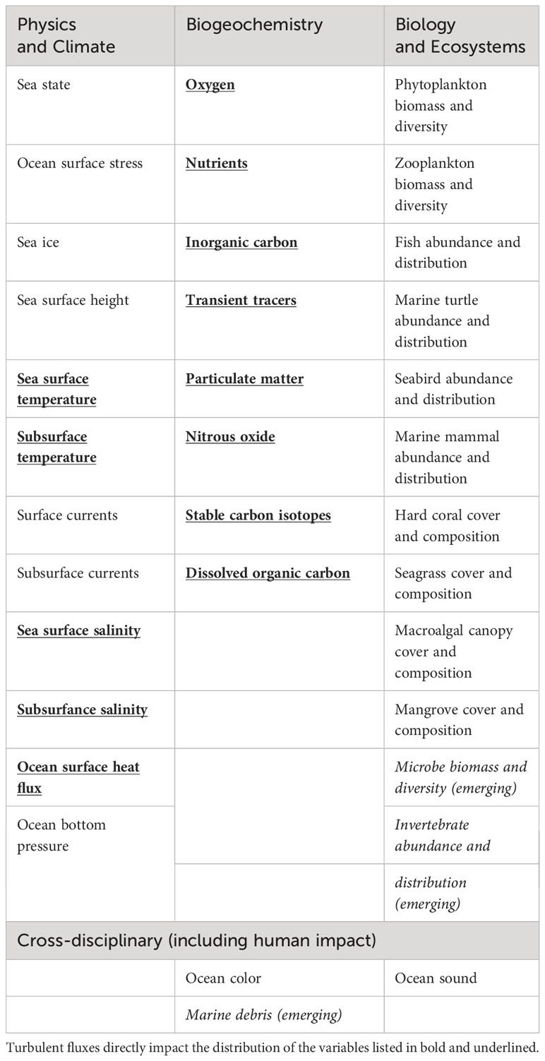
Table 2 Current list of Essential Ocean Variables.

3.2 Turbulent diapycnal fluxes as an Essential Ocean Variable

Our proposed variables (see Table 1) can be derived from the turbulent dissipation rate of kinetic energy (ϵ) and the turbulent dissipation rate of temperature (or another scalar) variance (χ), which are more easily measurable than direct covariance estimates from co-located velocity and tracer variance measurements (i.e., “eddy correlation” methods). Turbulent dissipation rates are obtained from measuring perturbations – ranging from a few centimeters to a few meters – of velocities and scalars such as temperature, conductivity (salinity), or dissolved oxygen. These variables are already part of the EOV list (Table 2), and ϵ is mentioned as a derived variable of Subsurface Currents in its EOV Specification Sheet. We argue, however, that GOOS should consider establishing an EOV specific to turbulent diapycnal fluxes for the following reasons:

1. Although turbulent diapycnal flux variables are related to existing EOVs (e.g., subsurface temperature and currents), they require different sampling protocols and instrument setups than traditional observations. Namely, selecting the time and spatial resolution depends on the turbulence theories invoked when deriving ϵ and/or χ from the observations, in addition to anticipated turbulence “energy” levels. The ultimate use for the observations also influences the choice of technique and sensors.

2. Turbulence variables depend on quadratic moments of existing EOVs at small spatial scales and fast time scales, so their calculation does not commute with averaging operations; crucially, this means that turbulence variables cannot simply be derived from existing EOV measurements, which sample at much lower frequencies and/or wavenumbers than needed to resolve J, ϵ, or χ (see Figure 3).

3. The EOV list should reflect the purpose of flux (J) or dissipation rate measurements (ϵ and χ) since they enable describing ocean dynamics beyond what can be documented from non-turbulent velocity and scalars. For instance, nutrient availability in the euphotic zone may be sporadically intense or input at a slower but more steady rate from turbulent exchanges. The magnitude of these turbulent exchanges, relative to other sources and sinks, cannot be gleaned solely by regularly monitoring currents and nutrients. Turbulent vertical fluxes may be the primary source for providing nutrients in the surface layer in many regions and they must be measured purposefully.

4. Global and sustained turbulent mixing observations are required to improve ocean mixing parameterizations in climate models. Ocean mixing is one of the three major uncertainties in climate models for sea level rise, along with ice sheet and cloud feedbacks (Melet and Meyssignac, 2015). Global climate models have begun using flow-dependent parameterizations for diffusivity, which require more direct diffusivity measurements to constrain them and assess the validity of their underlying assumptions.

Figure 3 From Bluteau et al. (2016b). Example spectral observations of shear spanning from ε ∼ 10⁻¹⁰ to ε ∼ 10⁻⁴ W kg⁻¹. The colored lines correspond to a theoretical shear spectra (e.g., Nasmyth spectrum) matching with the observations. Colored squares are placed at k_10, i.e., where 10% of the variance in the viscous range is resolved, while colored circles are placed at k₂₅. The thick lines delineate the wavenumber range that needs to be resolved to apply the integration method. The variance missing from the observation is corrected using the theoretical spectra. The bracket below the x-axis shows that the range of wavenumbers typically resolved by CTD and ADCP measurements is lower than the range required to resolve turbulent dissipation rates. A similar approach is used for the computation of χ with observed wavenumber spectra of temperature gradient matching the Batchelor spectrum. The reader should refer to the original study for the other features of the figure.

4 Measuring turbulent fluxes ($\overline{{\mathrm{U}}^{\prime }{C}^{\prime }}$) and turbulent diffusivity (K)

For turbulent diapycnal fluxes or mixing to occur, a source of energy must overcome the stable background stratification (e.g., through shear or convective instability) and create a growing overturning cell. A forward energy cascade occurs as the instability becomes non-linear and transitions to turbulence. As the cascade reaches scales where molecular processes become leading order, momentum, heat, salt, and passive tracers are diffused and get mixed between neighboring water masses, progressively lowering their total variance. In statistical equilibrium, the mean tracer variance $\overline{{(C^{\prime })}^2}$ is (on average) produced by fluctuating tracer fluxes acting upon mean gradients $\nabla \overline{C}$ at the same rate that it is dissipated by molecular diffusion:

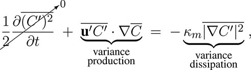(1)

where κ_m is the tracer’s molecular diffusivity and overbars denote averages. For the sake of simplicity, and mirroring the vast majority of previous ocean mixing studies, we have assumed here that the divergent transport terms can be neglected.

Turbulence is inherently a 3D process, but, at larger scales, it is constrained along isopycnals (approximately horizontal) by the overwhelming influences of rotation and stratification; only the relatively small, fast, and isotropic motions contribute to diapycnal (approximately vertical) fluxes. Thus, it is quite common to focus on the vertical component of Equation 1 which simplifies even further to

Here, w^′ and C^′ represent the microscale perturbations of vertical velocity and tracer concentration. In this formulation, the balance is between the average advective flux (i.e., turbulent diapycnal flux) of a tracer $(J_c\equiv \overline{w^{\prime }{C}^{\prime }})$ and the molecular dissipation of that tracer.

Focusing on the left hand side of equation 2, a bulk estimate of the turbulent diapycnal fluxes can be determined by invoking a Fick’s law approach, in which the flux is proportional to the concentration gradient of the tracer. The turbulent fluxes producing a tracer’s variance can be parameterized by the introduction of an effective turbulent diapycnal diffusivity K_C that shortcuts molecular dissipation by acting directly on mean tracer gradients, i.e.

The units of diffusivity are m²s⁻¹; it can be thought of as the rate at which the size of the tracer patch expands due to diffusion (Taylor, 1922; Ruan and Ferrari, 2021; Drake et al., 2022). While turbulent diffusivities can be separately defined for individual tracers (e.g., K_θ for potential temperature, K_S for salinity), it is often assumed that they are approximately equal in sufficiently turbulent environments – consistent with a mixing length argument (Prandtl, 1925).

The Fickian parameterization (equation 3) can be applied to the vertical fluxes of heat $(\rho c_p\overline{w^{\prime }{\theta }^{\prime }})$, salt $(\overline{w^{\prime }{S}^{\prime }})$ and any scalar $(\overline{w^{\prime }{C}^{\prime }})$, e.g., nutrients or dissolved gases (Gregg, 1987):

where J_q, J_S and J_C are the vertical fluxes of heat, salinity and a passive tracer C, respectively. This strategy enables the estimation of vertical fluxes for any parameter for which an accurate vertical gradient can be computed, provided K is known. There is no requirement to co-locate a fast-response sensor for the targeted parameter (e.g., oxygen) with a point-velocity sensor, which is the basis of existing “eddy correlation” field techniques (Pond et al., 1971; Lorrai et al., 2010; Bluteau et al., 2018).

Now focusing on the right hand side of equation 2, the molecular dissipation of a tracer can also be described by χ_C, which is the rate of dissipation of tracer variance, or the rate at which fluctuations in the tracer are smoothed out:

Using equations 2 and 3, the eddy diffusivity terms, K, can then be calculated directly from observations of χ:

with χ_θ and χ_S the dissipation of thermal and salinity variance, respectively. χ_C is the turbulent dissipation of tracer variance and quantifies the destruction of a tracer’s gradient through turbulence.

Similar relations can be derived for momentum from the turbulent kinetic energy equation (Osborn, 1980). Following the same assumption of statistical equilibrium and non-divergence of turbulent kinetic energy, the turbulent flux of momentum is balanced by the turbulent dissipation of kinetic energy ϵ and the turbulent buoyancy flux J_b, leading to:

with $N^2=-\frac{ɡ}{{\rho }_0}\frac{\partial \overline{\rho }}{\partial z}$ K_ρ as the turbulent diffusivity of buoyancy, and Γ as the mixing coefficient defined as a function of J_b and the momentum fluxes $\overline{w^{\prime }{u}^{\prime }}\frac{\partial \overline{\mathbf{u}}}{\partial z}$. In situations where temperature is the main control of the density distribution, it is possible to combine equations 4 and 8 to find that $\mathrm{\Gamma }=\frac{N^2}{2{\partial }_z{\overline{T}}^2}\frac{X_{\theta }}{\varepsilon }$. Typically, the mixing coefficient Γ is assumed to be ≈ 0.2 in the ocean, but its variability and dependence on flow properties remain the subject of continued research (Gregg et al., 2018). However, its variations are typically of order one, much less than the several orders of magnitude over which other turbulence quantities, such as ϵ and χ, vary in the ocean.

Turbulent flux equations (4) and (7) are simplified with diffusivity terms (6) and (8) by assuming that the production of variance is instantaneously balanced by the dissipation of variance (Osborn and Cox, 1972; Osborn, 1980). Although this assumption provides an indirect method of measuring turbulent diffusivities from ϵ or χ, values of K obtained in this manner are consistent with bulk diffusivities inferred from dye release experiments within accepted uncertainty ranges (Ledwell et al., 1998). Computing diffusivity by tracking dye provides a ground-truth of diffusivity, but measuring ϵ and χ is much more pragmatic for large-scale implementation in ocean observation networks.

As mentioned in section 3.2, measuring ϵ and χ requires data collection at centimeter-scale resolution or smaller. The required resolution cannot be obtain with most classic temperature, salinity and ocean velocity measurements, but with data collected at the appropriate resolution, ϵ and χ are “simply” the result of integrating the velocity and scalar (e.g., temperature) variations over the turbulence subranges – namely the inertial and the viscous subrange (Figure 3). The inertial subrange is a wavenumber band where the shear or temperature gradient increases toward smaller scale without being influenced by viscosity, and the viscous subrange corresponds to a wavenumber range where the signal is dissipated due to viscosity, creating a spectral roll-off. The shape and amplitude of the spectral signal can be modeled with theoretical spectra: the Batchelor spectrum for temperature gradient (Batchelor, 1959) and, among others, the Nasmyth spectrum for the shear (Nasmyth, 1970).

Practically, the integration of ϵ and χ is done assuming local isotropy, and integrating the one-dimensional spectrum in one direction, e.g., vertical direction for a vertical profiler or horizontal direction for a horizontal towed or moored sensor:

where ${\varphi }_{u_z}$ and ${\varphi }_{{\theta }_z}$ are the vertical (or horizontal) wavenumber spectra of velocity and temperature gradient (e.g., Lueck, 2022a, Lueck, 2022b), respectively. The spectra are integrated between k₀, the instrumentation-dependent lowest wavenumber accessible through the measurement observations, and k_c, a frequency cut-off separating the instrument noise from the signal. κ_T and ν are the thermal diffusivity and the kinematic viscosity, respectively. In the case of vertical profilers, we use the factors of 7.5 and 6 on the right-hand sides of Equation 9 and 10 to extrapolate the single observed dimension to three dimensions (note that these constants assume isotropic 3D turbulence).

Because ϵ and χ are spatial variance measurements, the sensors must record small variations in velocity and temperature within the microstructure range as a function of time while moving through the water. The time series can then be converted into spatial gradients using the mean flow passing the sensors. On profiling platforms, this is often taken as the instrument fall speed using the pressure data or nearby current data. Hence, measuring χ requires high-frequency thermistors (FP07) moving steadily through the water, i.e., a moving platform or flow passing through the sensor. Measuring ϵ can be done using shear probe (piezo-electric beams embedded in silicon) moving through the water, but is also achievable with other types of sensors and methods (Lueck et al., 2002; Le Boyer et al., 2021). For instance, ϵ can be determined from commercially available acoustic Doppler current profilers (ADCPs) using structure-function methods (e.g., Guerra and Thomson, 2017; McMillan and Hay, 2017), provided their sampling programs are specifically configured for turbulence measurements. Alternatively, point velocimeters that rapidly sample velocities at a fixed point in space can be used to obtain ϵ (Bluteau et al., 2011). Velocity-based methods typically rely on larger scales of turbulence within the inertial subrange, which are less taxing to measure but require the underlying assumptions in (9) to hold at larger scales. Hence, these techniques are typically limited to higher energy environments, but have the advantage of simultaneously providing information about the subsurface currents.

Applying eddy-correlation techniques to measurements from fast-sampling velocity-based instruments is the most direct way to obtain turbulent fluxes of a scalar (e.g., dissolved gases and salt). When paired with fast-response sensors such as dissolved oxygen (Bluteau et al., 2018) or temperature (Polzin et al., 2021), velocity-based instruments can be used to obtain turbulence quantities beyond ϵ and χ, such as the velocity-fluctuations (i.e., Reynolds stresses) or turbulent fluxes (〈w^′C^′〉). The scalar C^′ and the vertical velocities w^′ must be sampled sufficiently fast enough to resolve their time-averaged covariance over the flux-contributing time and length scales. In practice, this requires sensors that are sufficiently small and have response times of less than a second to measure the smallest flux-contributing scales while determining the largest flux-contributing scales to ensure the non-turbulent motions are excluded from the calculations (McGinnis et al., 2008; Lorrai et al., 2010). The relatively slow response times of most scalars (e.g., dissolved oxygen) hinder the application of the eddy-correlation method in high energy flows (high ϵ) because the flux-contributing scales are smaller with increasing ϵ. Because of these theoretical and technological difficulties, eddy-correlation methods have been limited to measurements from bottom landers in relatively quiescent environments; in particular, to examine near-bottom vertical fluxes of dissolved oxygen (e.g., Lorrai et al., 2010) and heat (e.g., Davis and Monismith, 2011). These difficulties are the reason that the scientific community has focused on collecting bulk turbulent flux measurements through ϵ and/or χ, rather than direct turbulent flux measurements.

Other methods also exist to estimate ϵ, which rely on even larger scale measurements than the velocitybased techniques above. Although easier to measure, they come with larger biases than measuring ϵ from shear probes or fast-sampling velocities. For example, using lower-resolution density profiles, ϵ can be computed from Thorpe scale overturns at meters scales. Thorpe scales highlight gravitationally unstable regions of the water column, indicating turbulence (Mater et al., 2015) with the caveat that, to do so, the overturn is assumed to be fully turbulent, which is not always the case and can induce bias in the estimation of ϵ. Alternatively, finescale parameterizations can also be used from lower resolution observations of shear, strain or kinetic energy (Polzin et al., 1995; Polzin et al., 2014; Whalen et al., 2015). Parameterizations estimate ϵ by comparing the observed internal wave field characteristics (e.g., shear, strain) with the Garrett and Munk spectrum – a description of an average internal wave field (Garrett and Munk, 1972). These estimates are known to differ by order of magnitude or more at some locations in the deeper ocean (Figure 4, Klymak et al., 2008; Waterman et al., 2014). Parameterizations rely on the assumption that most mixing is driven by internal waves, and is only applicable in the open ocean (Polzin et al., 2014). Until parameterizations can be built for more specific cases, there will always be a discrepancy between parameterized and measured turbulence values at ocean boundaries.

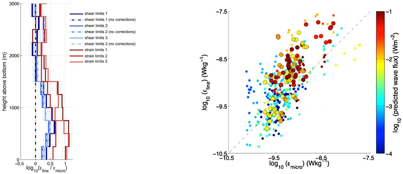
Figure 4 Evidence of discrepancies between fine-scale parameterization and direct observation from Waterman et al. (2014). Left: A comparison of the station-averaged vertical profiles of ϵ_fine/ϵ_micro (finescale parameterization for ϵ/measured microstructure ϵ) ratio as a function of height above the bottom for various implementations of the finescale parameterizations. The strain parameterization (red lines) is the only one that can be used with Argo float data. Right: Scatterplot of log₁₀(ϵ_micro) versus log₁₀(ϵ_fine) colored by the local predicted lee-wave energy flux.

5 Instrumentation maturity

Turbulence measurements require a high sampling frequency compared to the other EOVs. In this section, we present existing instrumentation allowing for the computation of ϵ or χ (section 5.1), for the direct measurement of turbulent fluxes (section 5.2, or for the integration of both methods on a single platform 5.4).

5.1 Microstructure-based measurements

The first in-situ observations of ocean turbulence were made by researchers at the Pacific Naval Laboratory of Canada’s Defence Research Board using hot film anemometers (Grant et al., 1962). Since then, the ocean mixing community has continued to design and improve instruments that are increasingly resilient and easy to deploy. The rapid evolution of instrumentation has enabled more autonomous measurements and the mobile electronics industry has progressed tremendously over the past decade, reducing the size and power of electronic components while increasing data storage capacity. The types of platforms used to measure turbulence have expanded from profilers and towed vehicles to moorings, gliders, AUVs, autonomous profilers, and Argo floats.

The basic sensor technology available to make direct mixing observations in the microstructure range has been in place since the 1970s (see exhaustive review by Lueck et al., 2002). Airfoil shear probes and FP07 thermistors sample small-scale gradients of velocity and temperature, respectively, at frequencies of 100-512 Hz, which equates to a spatial resolution of centimeters. FP07 thermistors and shear probes each have advantages and disadvantages for measuring turbulence. Shear probes measure small-scale velocity fluctuations, directly measuring the loss of kinetic energy associated with turbulent motions. FP07 thermistors measure small-scale temperature fluctuations and thus provide an indirect measurement of how turbulent motions affect background temperature gradients. Shear probes are more sensitive to platform speeds and vibrations than FP07 thermistors. Conversely, thermistors have a slower response time, limiting their ability to resolve the smallest eddies in areas of strong turbulence at reasonable fall speeds. Both types of sensors are very delicate and can be damaged if they encounter large zooplankton in the water column. A new type of plastic membrane (e.g., polyvinylidene fluoride, PVDF) with similar piezo-electric properties to the currently used ceramic materials has the potential to greatly improve the resilience of shear probes over the next five years. These plastic membranes are flexible and, therefore, more resilient to shocks and pressure forces.

Since the early turbulence measurements, the sensors themselves have not changed significantly, but the electronics and data acquisition systems have improved resulting in higher signal-to-noise ratios and reduced power consumption. Onboard data storage has also increased significantly, allowing the on-board processing of the turbulent dissipation rates (ϵ,χ). Autonomous platforms (e.g., gliders and floats) already use on-board processing schemes (e.g., Hughes et al., 2023). Using vibration sensors and data processing algorithms has also reduced signal contamination from sources such as platform vibrations (Goodman et al., 2006). One can also rely on the larger scales of the microstructure subrange to estimate ϵ (Bluteau et al., 2016b) and χ (Bluteau et al., 2018) to avoid vibration issues by sampling less rapidly. Furthermore, progress has been made in estimating the statistical uncertainty of a dissipation estimate and the quality of a spectrum objectively (Lueck, 2022a,b), which allows automated and reliable quality control of dissipation estimates. These improvements, combined with the recent progress in real-time data processing, have 1) allowed more compact instruments to be built, 2) enabled the transmission of data over satellite connections, and 3) allowed for instruments to be deployed for longer periods (e.g., Rainville et al., 2017). They also enable more data to be recovered from autonomous platforms deployed in high-traffic areas where platforms are sometimes damaged or lost.

5.2 Velocity-based measurements and platforms

Acoustic-Doppler Current Profilers (ADCPs) and point-velocity measurements are instruments routinely deployed on bottom landers and moorings. Estimating ϵ from these sensors requires measuring velocities at a sufficiently high rate to sample within the inertial subrange (seconds and several cms). The point-velocity measurements are more mature than using ADCPs to obtain ϵ as it relies on fitting the inertial subrange of spectra derived from time-series over a small sampling volume of a few centimeters. The first estimates of ϵ were from electro-magnetic sensors (Bowden and Fairbairn, 1956) or drag spheres (Lumley and Terray, 1983) until acoustic-Doppler velocimeters with sufficiently low measurement noise became common in the late 1990s (e.g., Voulgaris and Trowbridge, 1998; Kim et al., 2000). Initially, turbulence estimates were only possible from fixed platforms since high-frequency platform motion (e.g., vibrations) could not be easily removed from the velocity signals. Over time, techniques to handle the changes in expected spectral forms from surface waves were generalized (Lumley and Terray, 1983; Feddersen et al., 2007), while reducing the impact of motion contamination on moored point-velocity measurements (e.g., Bluteau et al., 2016a).

The use of ADCPs to derive ϵ, can provide estimates over a wider range of depths than one point-velocity meters. The technique was first introduced by Wiles et al. (2006) and relies on the structure-function first employed in meteorology in the late 1960s (Sauvageot, 1992). Deriving ϵ requires differencing instantaneous turbulent velocities at different separation distances along an ADCP beam. As with the point-velocities, the sampling rate must be sufficiently fast to measure within the inertial subrange (1-2 Hz typically). The noise and measurement quality must be much higher than for measuring mean currents, and so the ADCPs must be programmed in pulse-to-pulse coherent mode. This mode results in higher resolution measurements but over a small spatial range of typically less than 10m. The method also requires that the bin separation is sufficiently small so that a few bins are fully contained within the inertial subrange. For relatively weak turbulence levels of ϵ ∼ 10⁻⁸ Wkg⁻¹, a bin size of 20cm is sufficiently small. In more energetic flows, the inertial subrange extends to smaller scales but also to larger scales such that the bin size does not need to be reduced at the expense of the ADCP’s vertical sampling range.

Several commercial offerings currently exist to measure ϵ over a wide range of turbulence levels and spatial scales with the structure-function. For example, the structure-function has been applied to ADCPs available from Nortek and RDI Teledyne (see Guerra and Thomson, 2017, for comparisons between instruments). The structure-function method was been applied to moored ADCPs using off-the-shelf instruments (Lucas et al., 2014). Velocity profiles of sufficient quality for turbulence analysis are also possible from off-the-shelf instruments mounted on Lagrangian (drifting) floats (Shcherbina et al., 2018).

Another type of acoustic measurement uses travel-time velocimeter technology (TTV, Polzin et al., 2021). Similar to the point velocities, TTV instruments measure a small volume of water using a pair of transducers “pinging” at each other. This technology allows for a very fast sampling in low-scattering environments and can be used for direct observation of turbulent fluxes (eddy-correlation methods). The eddy-correlation method is relatively new in the deep ocean science community and requires a time-scale separation that could lead to bias in the turbulent fluxes computation.

5.3 Platforms

Microstructure measurements have been made using several different instruments mounted on a variety of platforms (Figure 5). The first measurements were made using horizontal profilers that were towed by a ship (e.g., Grant et al., 1962). By the late 1970s, most microstructure measurements were made using vertical profilers developed by over 10 different research groups around the world (Lueck et al., 2002). Currently, microstructure instruments are made commercially by Rockland Scientific International (Canada) and Sea and Sun Technology (Germany), and by research groups at Oregon State University (OSU), Scripps Institution of Oceanography (SIO), and Woods Hole Oceanographic Institution (WHOI).

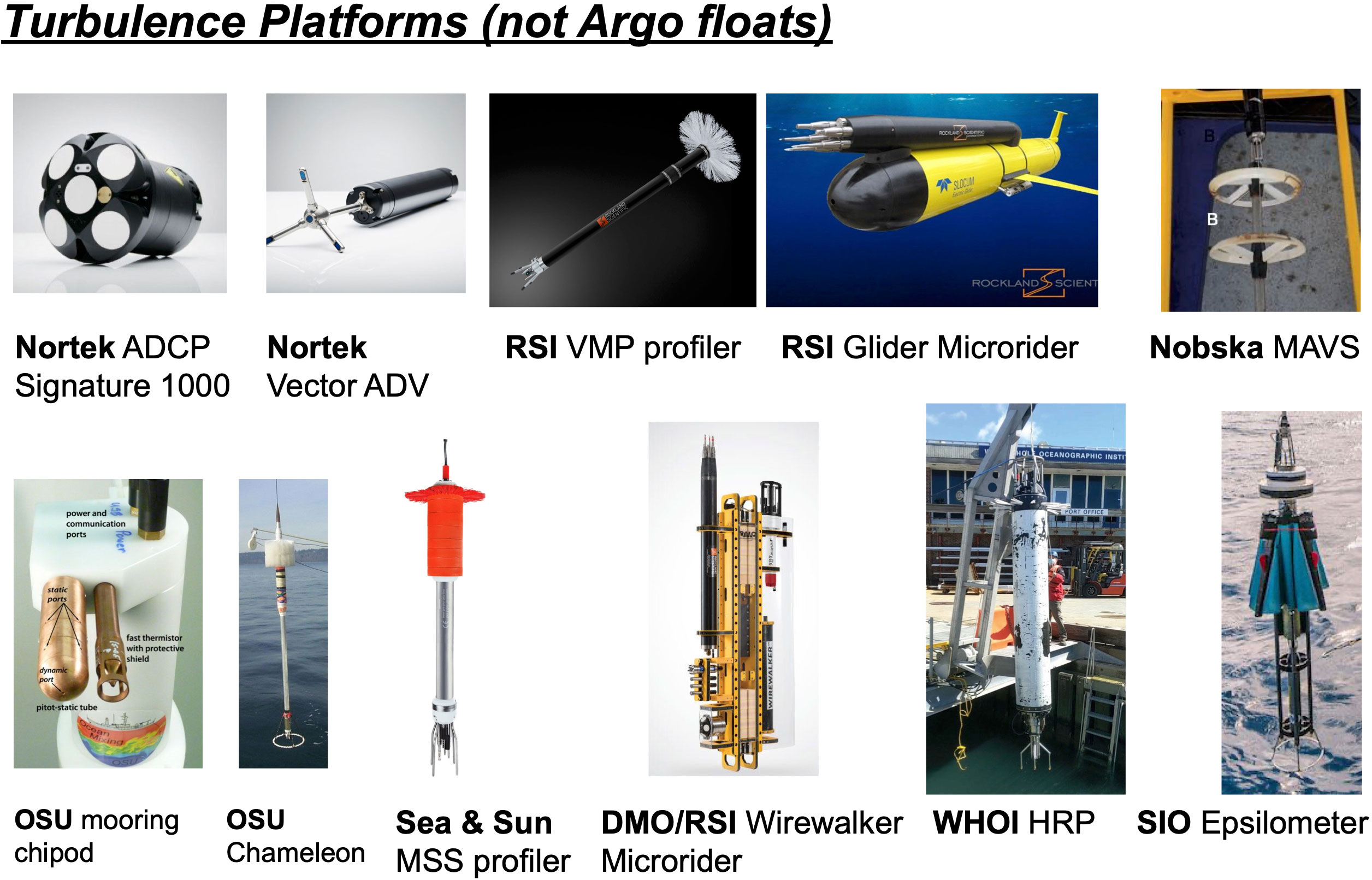
Figure 5 Examples of platforms measuring ϵ, χ or turbulent fluxes directly.

Most of these instruments are designed to make simultaneous measurements of both shear and temperature microstructure from vertical profilers (autonomous or tethered) for a variety of depth ratings (up to 11,000m) and modular instruments that can be mounted on autonomous platforms such as gliders, AUVs, and drifting or moored profilers (e.g., Argo floats or Wirewalkers). Vertical profilers remained the dominant method of obtaining microstructure measurements until the 2010s, when instruments began to be mounted on moorings, gliders, AUVs, and surface-following platforms (e.g., Moum and Nash, 2009; Fer et al., 2014; Hughes et al., 2020; Iyer et al., 2021; Zippel et al., 2021). These new platforms, combined with more versatile instruments, have led to a significant increase in the volume of data being collected and the duration of deployments. Deployments on autonomous platforms are power-limited and typically last up to 45 days. This equates to 300 glider profiles to 1000m.

Longer turbulence deployments are possible from moored platforms, although measurements are limited to discrete depths rather than the full water column. χpods, which contain FP07 sensors mounted horizontally, have provided near-continuous mixing measurements at the equator on several of the Tropical Atmosphere–Ocean (TAO) array moorings since late 2005 (Moum et al., 2013) in the Pacific Ocean, and later in the Atlantic Ocean (PIRATA array) and Indian Ocean (RAMA array). The TAO/TRITON (Triangle Trans-Ocean Buoy Network) program evolved from the original TAO project started in 1985 and was sponsored by CLIVAR, GOOS, and SCOR (https://www.pmel.noaa.gov/gtmba/, McPhaden et al. (2010)). PIRATA launched in 1997 (Bourlès et al., 2008), RAMA evolved from the Indian Ocean Observing System (IndOOS) with original deployment in 2006 (McPhaden et al., 2009; Beal et al., 2020). Only a few sensors allowing for direct measurements of turbulent fluxes (e.g., MAVS Figure 5 using TTV technology) can be mounted on mooring and record velocity-tracers fluctuations over a wide range of frequencies.

CTD-χpods – an adaptation of χ-pods suitable for mounting on a standard rosette (Figure 6) – have been deployed on cruises that are part of the international GO-SHIP Repeat Hydrography Program since 2014. Through this effort, CTD-χpods have provided χ and turbulence measurements across sections in the Pacific, Atlantic, Indian, and Arctic Oceans with the intent to obtain repeated full-depth measurements on a global scale.

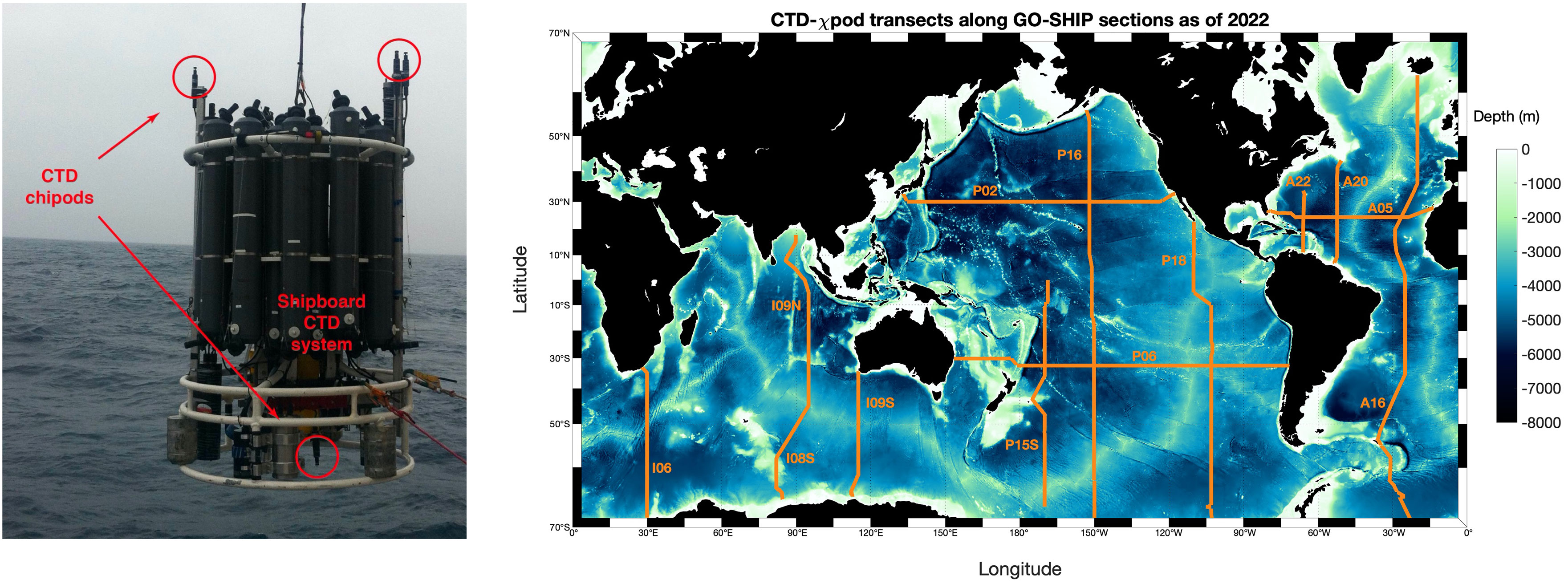
Figure 6 Left: CTD-rosette equipped with CTD-χpods deployed during a recurrent GO-SHIP transect. Right: CTD-χpod transects as of 2022.

5.4 Argomix

One of the most relevant programs to our discussion is the international Argo program, which collects ocean data using a fleet of autonomous instruments that drift with the ocean currents and move up and down between the surface and a mid-water level. The Argo floats are part of a global coordinated effort of over 30 nations with more than 3500 autonomous ocean-observing profilers currently active in the network (http://www.jcommops.org/). The floats provide the scientific community with near-real-time ocean measurements including temperature and salinity profiles, so they are already an important platform for physics EOVs. The ongoing integration of turbulence sensors on Argo floats has the potential to provide turbulent dissipation rate measurements on a daily basis at a global scale. The present discussion recognizes the need for the ocean mixing community to further coordinate its efforts to measure and distribute data, taking advantage of the means provided by the GOOS.

Mixing measurements from Argo floats (Argo-mix) are one of the emerging branches of the Argo program (Roemmich et al., 2019). This new branch, will provide the scientific community repeated microstructure measurements at a global scale. These measurements would offer insights into the impact of ocean mixing on water mass transformations, air-sea interactions and a plethora of other processes (Naveira Garabato and Meredith, 2022). Technological improvement needs to provide resilient and low-power new sensors so their integration does not modify the life expectancy or the core mission of a float– namely long-term deployments profiling the upper 2000 m.

An early effort obtained more than 1000 profiles over two weeks in the Bay of Bengal from two χSOLO floats, which are Argo floats equipped with fast thermistors (Shroyer et al., 2016). This instrument motivated development of the Flippin’ χSOLO (FCS), which has shear probes and fast thermistors at one end of the float and a communication antenna at the other (Moum et al., 2023). By flipping around at the top and bottom of a cast, turbulence profiling of undisturbed fluid is achieved on both down- and up-casts all the way through the sea surface. Similar to glider performances, FCS missions can last 45 days when profiling to 120m at a rate of roughly 100 profiles per day. Missions are controlled from a shore station by remote communications.

While χSOLOs have reached a mature level of operation, additional microstructure floats are under development (Figure 7). The microstructure sensors developed by Rockland Scientific International and SIO are currently being integrated in the MRV ALTO and APEX floats, respectively. Both of these floats are part of the Argo fleet. The deployments of these floats began in 2022 during a few pilot experiments that profiled to 2000 m. The first results show a good sensitivity range despite the slow motion of the floats. The integration of these turbulence sensors on Deep-SOLO floats – Argo float profiling down to 6000 m depth – is also underway. The probes used on the sensors are expected to survive the challenging pressure at such a depth since they show normal sensitivity and behavior after multiple bench-tested pressure cycles up to 10000 PSI (>7000 m depth).

Figure 7 Examples of Argo floats equipped with microstructure packages: An Apex float from the University of Washington with an Epsilometer from SIO (Left), A MicroAlto float from MRV equipped with a Rockland MAPLe™ (middle) and a SOLO float equipped with turbulence sensors from Oregon State University.

A new project from the National Oceanographic Partnership Program (NOPP) aims to improve the global simulation of internal waves and their impacts on ocean mixing. As part of this effort, the SQUID (“Sampling QUantitative Internal-wave Distributions”) sub-project sponsored by NSF will deploy 50 EMAPEX microstructure floats measuring velocity, temperature, salinity, and χ from cruises of opportunity throughout the world in 2023–2025 (Figure 8). Sampling will differ from the Argo paradigm by making bursts of 4-6 profiles to 2000 meters over two days, allowing the estimation of a statistical average and high-frequency perturbations in shear, strain, and dissipation, as well as energy flux by dominant internal wave components through low-mode fitting and harmonic analysis. Bursts will be separated by multi-day drifting at 1000m, with a target duration of one year per float. The overall SQUID array, while not covering the globe by any means, will aim to span the range of major internal wave forcing parameters (including internal tide amplitude as estimated from altimetry, bathymetric roughness, high-frequency wind forcing, mesoscale eddies, and latitude).

Figure 8 Map of possible deployment sites for 50 EM-APEX floats from cruises of opportunity in 2023 2025. These floats make up the SQUID (Sampling QUantitative Internal-wave Distributions) contribution to the NOPP Global Internal Waves experiment, aimed at validating internal wave models and their implications for mixing by internal waves. Courtesy of James Girton, APL-UW.

5.5 Error bar and uncertainties

Practical measurements of ϵ (and fluxes derived from these) have unavoidable uncertainties. Even an instrument with multiple (redundant) sensors will not necessarily produce the same values. Further, turbulence has short spatial and temporal scales and therefore point measurements are not necessarily representative of that part of the ocean on longer (e.g., >weekly) or larger (e.g., >10km) scales and requires multiple realizations to address the time and space variability turbulent diapycnal fluxes.

Lueck (2022a) showed that ϵ values measured by individual shear sensors on the same instrument agree in an average sense but that there is typically variability up to a factor of two. Specifically, for 90-cm segments, agreement between sensors was worse than a factor of two in 10% of cases. Shorter segments have larger variability and longer segments have smaller variability. Similar levels of agreement are described by Oakey (1982) who compared ϵ derived from a shear probe to that derived from a thin film thermometer, and by Kolås et al. (2022) who compared outputs from two shear probes installed on an AUV. (Further examples are given in Section 3.1 of the turbulence methodology review by Burchard et al. (2008)).

Averaged over hours to days, turbulence measurements from independent instruments—but from the same nominal part of the ocean—should give the same results. Moum et al. (1995) tested this with two free-falling profilers from two ships spaced within 11km of each other on the equator (0°, 140°W). At most depths, the agreement between the full 3.5-day means were within a factor of two. Agreement between individual data pairs was typically within a factor of three but sometimes beyond a factor of 10. In other words, the natural variability of geophysical turbulence over kilometer scales is comparable to, or larger than, the uncertainty associated with each point measurement of ϵ.

Clearly, if turbulence measurements at a given spot are to be considered representative, averaging is needed and/or uncertainty levels need to be quantified. As with any measurement, but especially for turbulence, more samples are better for achieving accurate statistics. Observed distributions of ϵ are often approximately lognormal. Hence, distributions of log(ϵ) are approximately Gaussian, which makes standard statistical quantities such as mean and standard deviation easy to calculate (e.g., Baker and Gibson, 1987). However, one can avoid assuming a Gaussian distribution by using bootstrapping, a statistical method that is agnostic to distribution shape. Indeed, bootstrapping is a standard procedure in turbulence analysis (e.g., Shay and Gregg, 1986; Lu et al., 2000; Greenan et al., 2001; Nash and Moum, 2001; Inall and Rippeth, 2002; Klymak and Moum, 2007; St Laurent and Thurnherr, 2007; Perlin and Moum, 2012; Whalen et al., 2012; Sutherland et al., 2013; Waterhouse et al., 2014; Wenegrat and McPhaden, 2015).

This discussion of uncertainties, which so far only considers ϵ, can be extended to turbulent fluxes, albeit with caution. As Moum (1997) emphasizes, microstructure measurements are not flux measurements, and the assumptions linking the two are ‘fraught with uncertainty’. That said, direct numerical simulations show that the Osborn and Cox (1972) and Osborn (1980) relations outperform their underlying assumptions in predicting diffusivity and hence the irreversible buoyancy flux (Taylor et al., 2019). This is consistent with the widely held notion from observations that Γ = 0.2 (see Gregg et al., 2018, and elsewhere in this paper).

6 Data processing and international coordination

The ocean mixing community is increasingly committed to integrating observation efforts and standardizing methods for data quality control and distribution. An archive for turbulence data is maintained by the CLIVAR’s Carbon Hydrographic Data Office (microstructure.ucsd.edu). This database was created by the Climate Process Team (CPT), funded by NSF and NOAA between 2010 and 2015. The team’s mission was to develop and test mixing parameterizations for climate models. To this end, they created an archive for turbulence data that compiles processed datasets of dissipation rates from research programs in a single repository. The format of the data included in this archive is standardized so that observed turbulent dissipation rates can be easily incorporated into models or process studies.

Creating a common dataset is a complex undertaking due, in part, to the sensitivity of the observed dissipation rates to the different algorithms independently developed and customized for the different platforms (up to five in the CPT database). The ATOMIX working group was founded in 2020 to establish a consensus regarding best practices for the derivation of ϵ from observed shear microstructure and acoustic measurements. These efforts come on the heels of a nearly 20-year history of official coordinated efforts of the ocean mixing community; a prior SCOR working group (Working group 121) began in 2002 with a goal to summarize the state of knowledge about ocean mixing and to identify the steps that would be required to improve mixing parameterizations in global climate models. Going forward, ATOMIX will establish and communicate measurement standards through a wiki and propose a set of validated data to build calibrated global turbulence measurements.

7 Feasibility and cost effectiveness

Besides the scientific relevance of observing subsurface turbulent fluxes at a global scale, the feasibility and the cost-effectiveness of these measurements are two of the main criteria that must be met to show that turbulent fluxes belong in the EOV list. In the EOV context,

● Feasibility implies that observing or deriving turbulent fluxes on a global scale is technically feasible using proven, scientifically understood methods.

● Cost effectiveness means that generating and archiving turbulence data is affordable, mainly relying on coordinated observing systems using proven technology, taking advantage where possible of historical datasets.

7.1 Feasibility and pilot programs

The TAO and CTD-χpods projects mentioned earlier have demonstrated the feasibility of collecting basinwide datasets of microstructure observations (Figure 6). These projects integrated turbulence measurements into the structure and culture of repeat hydropgraphy cruises and developed a methodology for processing and interpreting the acquired ocean mixing data. CTD-χpods are also being tested in coastal environments to possibly widen the scope of their usage. Expanding to global observations is a matter of putting more instruments in the ocean.

Measurements of ϵ are reaching a similar level of maturity within the Argo-mix context and the ongoing integration of turbulence packages measuring ϵ and χ inside Argo floats. The float controls a unique low-power electronic board that can collect data from analog channels and has the required memory space to compute the dissipation rates and a few quality flags. Such packages, as well as the use of easy-toreplace shear and FP07 probes, simplify the integration of microstructure sensors greatly. Once they are an integrated part of the Argo fleet, microstructure measurements at a global scale will automatically be available to a wide community. Before their full integration, a few regional pilot experiments (e.g., the SQUID project mentioned in section 5.4) will be performed to validate and prove that measurements from autonomous Argo floats are fit-for-purpose.

The recent success of the biogeochemical community in incorporating sensors onto global observation platforms like Argo floats can be used as a roadmap for the ocean mixing community. Autonomous floats or vehicles able to sample the turbulent fluxes and diffusivities during the lifetime of coherent oceanic structures (e.g., mesoscale eddies or equatorial cold tongue) can provide insights about local energy transfers inside structures impacting the global circulation. The scales (time and space) of these structures makes them ideal candidates for pilot experiments that will demonstrate that Argomix floats are also fit-for-purpose of the core Argo mission.

Argomix floats, ϵ measurements from already existing platforms (e.g., gliders, profilers, high-resolution ADCPs or ADVs), and current efforts to develop a consistent methodology for processing and interpreting measurements (e.g., ATOMIX SCOR group) all converge toward integrating turbulent flux observations into the structure and culture of repeated hydrography cruises and observing systems.

7.2 Cost-effectiveness

The cost-effectiveness of repeated microstructure measurements represents a balance between 1) the price of the turbulence sensors, 2) the cost of the platforms used for these measurements and 3) the funds dedicated to coordinate observing systems and ship opportunities in charge of maintaining these measurements. Over the past 40 years, many regional research projects have been funded by national research agencies in attempts to quantify turbulent dissipation (Waterhouse et al., 2014). Regional scale experiments provide high-resolution time series of ocean turbulence that shed light on its variability and the multi-scale interaction between ocean energy sources and energy dissipation. Understanding these interactions is of primary importance for future human activities (e.g., deep sea mining, energy harvesting, sea level rise). As the connection between ocean mixing and human activities has become more apparent, private organizations have begun supporting studies that include microstructure measurements (e.g., Schmidt Family Foundation and the Benioff Foundation, Muñoz-Royo et al., 2021). In 2018, the physical oceanography program at NASA identified ocean mixing as one of its three priority areas and funded several projects, including efforts associated with the χ measurements made on the international GO-SHIP hydrography program, described above.

The cost of autonomous platforms like Argo floats spans from $20k for a core (Temperature-SalinityPressure) float to about $100k for a biogeochemical Argo float with six additional sensors. As of today, the microstructure packages considered for the Argo float integration range around $30k–$40k in their current form. Progress in the electronics industry is triggering the development of new generations of turbulence sensors and new fabrication techniques are lowering the fabrication cost of these packages by a factor of three (Le Boyer et al., 2021). This will bring the cost of an “Argomix” float well within the price range of a core Argo float and a biogeochemical float. The necessary simplification of turbulence packages to fit into the tight space of the float, as well as any production scaling, will further reduce the price of Argo-mix floats.

Consequently, the ocean mixing community will be able to design regional scale experiments with sampling strategies using a small fleet of ∼10 microstructure sensors measuring both ϵ and χ from a variety of easy-to-deploy platforms with a<$500k budget within the next five years (e.g., SQUIDD project mentioned above).

8 Conclusions

Currently, global climate models do not resolve turbulent mixing, and instead use turbulent diffusivity schemes to parameterize turbulent fluxes using the physics of processes (e.g., internal waves, mesoscale and submesoscale processes) that are thought to drive part of the ocean mixing. In regions where turbulent production is dominated by the internal wave field, the finescale parameterization can be used to predict the patterns of ocean mixing based on the resolved model state. However, strong ocean mixing signals occur near the boundaries (surface and bottom) and in regions where mesoscale and submesoscale processes are important. The dynamics of these processes modify the internal wave field and violate the assumptions required to use the parameterization. As a result, models poorly represent ocean mixing where it matters the most, and the turbulent diffusivity scheme needs to be improved by observational inputs.

Not only are parameterizations of ocean mixing failing to estimate dissipation rates in key regions, but evidence is mounting that the picture drawn in the 1960s, presenting turbulent diffusivities as a largely dynamically passive phenomenon, does not provide an adequate explanation of many climatically important aspects of the ocean’s behavior. Major elements of the oceanic circulation are governed by dynamic interactions between ocean mixing processes and the large-scale ocean state, and are thus not well captured by the current generation of state-of-the-art Earth system–class ocean models. The conclusion seems inevitable that to generate a step change in our understanding and modeling capability, sustainable and global turbulence observations are required to describe and quantify the circulation-shaping role of ocean mixing (Naveira Garabato and Meredith, 2022).

The instrumentation for such observations has been developed since the 1960s and recently benefited greatly from the mobile technology revolution and the chip-miniaturization that went with it. Storage capacity, processing speeds and reduced power consumption allow for cheaper and modular instruments that can be embedded in autonomous platforms like Argo floats, gliders or AUVs. With their extended range and life expectancy, these platforms can now be used for large-scale and long-term experiments. The obvious and on-going next step for the ocean mixing community is to develop methods and coordinate efforts between research groups to ensure the creation of a sustained global observing system for mixing (Naveira Garabato and Meredith, 2022). The instruments and platforms mentioned in this document can be sorted, using the UNESCO readiness level grid, in terms of maturity for being deployed on a global scale. All of them are past the proof of concept level and are deployed in the context of pilot experiments (Figure 9).

Figure 9 Levels of maturity of turbulent diapycnal flux observations mapped onto the EOV framework: Requirements (i.e., instrumentation, Methods), Coordination (i.e., strong community) and Data management (i.e., database and processing best practices). The Framework for Ocean Observing evaluates possible new components to be included in the Global Ocean Observing System (GOOS) based on their readiness level (UNESCO, 2012). A variable in levels 1-3 is identified as societally important and observations have been made at basin scale levels. A variable in levels 4-6 has a verified sampling strategy with autonomous deployment and international collaboration. A fully mature variable is validated through peer review and has sustained measurements at global scales. Data products are routinely publicly available. Turbulent diapycnal fluxes fall in the range of “Pilot” level maturity (Levels 4-6), during which instruments and coordination are tested and made ready for large-scale implementation. The components are well on their way to the “Mature” range of readiness (Levels 7-9).

A number of initiatives and experiments participate in that goal. The Scientific Committee on Oceanic Research is supporting ATOMIX, a working group creating a universal set of standards for measuring and distributing ocean mixing data with appropriate quality control flags. Similarly, the National Science Foundation and National Oceanic and Atmospheric Administration supported the climate process team on internal-wave driven ocean mixing, which improved diffusivity parameterizations in global climate models (MacKinnon et al., 2017). A consequence of these efforts to coordinate research groups was the creation of an ocean turbulence database (Waterhouse et al., 2014). Along with these community efforts to centralize and standardize data production, sustained large-scale observation programs, like GO-SHIP and the Argo program, have either already integrated or are currently integrating turbulent mixing instrumentation.

Several research groups and companies are currently working on the integration of turbulent sensors in the Argo program. Floats with integrated turbulence packages are already part of regional experiments (Shroyer et al., 2016). The engineering challenges of sensor resilience, energy consumption and costs are being overcome thanks to new technologies and materials. At the time of writing, the turbulence sensing community is about five years away from producing instruments that can be easily deployed and survive hundreds of profiles, collecting quality-controlled estimates of ocean mixing. Keeping the pace of current development, major programs (e.g., Argo, NASA) are acknowledging that ocean mixing is relevant to climate and ocean health, as discussed in Section 1. Consistent global scale measurements will have an positive impact on the reliability of global climate models, our understanding of global circulation patterns, and our ability to map and predict physical, chemical, and biological parameter distributions on regional and global scales. As feasibility challenges are overcome through emerging technologies and the cost per unit comes down, the inclusion of ocean turbulent mixing as an Essential Ocean Variable should be on the horizon.

Author contributions

Lead authors AB and NC, designated by the symbol “*” and listed first in the list of authors, had primary responsibility for writing all sections of the manuscript. The other co-authors contributed in the following: Introduction – All co-authors with strong participation from HD, KH, CB; section 2 – HD, KH, CB, AN, MM, IF; section 3 – HD, CB, AN, TP, EF, AMa, LC, AMe, IF; section 4 – CB, KH, MA, CS, MD, IF; section 5 – MA, CB, IF, MD, AMo; section 6 – CB, KH, AMo; section 7 – AN, CB, AMo; Conclusion: All co-authors. All authors contributed to the article and approved the submitted version.

Funding

The author(s) declare that no financial support was received for the research, authorship, and/or publication of this article.

Acknowledgments

All co-authors, and especially the lead authors acknowledge the tremendous input from J. Moum who helped re-oriented the main topic of this white paper toward what the ocean community is now considering the best option for turbulence data to become an EOV. We are also in debt of all the pioneers who participated in the development of today’s turbulence technology.

Conflict of interest

The authors declare that the research was conducted in the absence of any commercial or financial relationships that could be construed as a potential conflict of interest.

Publisher’s note

All claims expressed in this article are solely those of the authors and do not necessarily represent those of their affiliated organizations, or those of the publisher, the editors and the reviewers. Any product that may be evaluated in this article, or claim that may be made by its manufacturer, is not guaranteed or endorsed by the publisher.

References

Adcroft A., Anderson W., Balaji V., Blanton C., Bushuk M., Dufour C. O., et al. (2019). enThe GFDL global ocean and sea ice model OM4.0: model description and simulation features. J. Adv. Modeling Earth Syst. 11, 3167–3211. doi: 10.1029/2019MS001726
Baker M. A., Gibson C. H. (1987). Sampling turbulence in the stratified ocean: statistical consequences of strong intermittency. J. Phys. Oceanogr. 17, 1817–1836. doi: 10.1175/1520-0485(1987)017<1817:STITSO>2.0.CO;2
Batchelor G. (1959). Small-scale variations of convected quantities like temperature in turbulent fluid. J. Fluid Mech. 5, 113–133. doi: 10.1017/S002211205900009X
Beal L. M., Vialard J., Roxy M. K., Li J., Andres M., Annamalai H., et al. (2020). A road map to IndOOS-2: Better observations of the rapidly warming Indian Ocean. Bull. Am. Meteorol. Soc. 101, 1891–1913. doi: 10.1175/BAMS-D-19-0209.1
Bindoff N., Cheung W., Arístegui J., Guinder V., Hallberg R., Hilmi N., et al. (2019). Chapter 5: Changing ocean, marine ecosystems, and dependent communities, IPCC special report oceans and cryospheres in changing climate eds. Pörtner H.-O. D., Roberts C., Masson-Delmotte V., Zhai P., Tignor M., Poloczanska E., et al (Cambridge, UK and New York, NY, USA: Cambridge University Press), 447–587.
Bluteau C. E., Galbraith P. S., Bourgault D., Villeneuve V., Tremblay J.-É. (2021). Winter observations alter the seasonal perspectives of the nutrient transport pathways into the lower St. Lawrence estuary. Ocean Sci. 17, 1509–1525. doi: 10.5194/os-17-1509-2021
Bluteau C. E., Ivey G. N., Donis D., McGinnis D. F. (2018). Determining near-bottom fluxes of passive tracers in aquatic environments. Geophysical Res. Lett. 45, 2716–2725. doi: 10.1002/2017GL076789
Bluteau C. E., Jones N. L., Ivey G. N. (2011). Estimating turbulent kinetic energy dissipation using the inertial subrange method in environmental flows. Limnol. Oceanography: Methods 9, 302–321. doi: 10.4319/lom.2011.9.302
Bluteau C. E., Jones N. L., Ivey G. N. (2016a). Acquiring long-term turbulence measurements from moored platforms impacted by motion. J. Atmos Oceanic Technol. 33, 2535–2551. doi: 10.1175/JTECH-D-16-0041.1
Bluteau C. E., Jones N. L., Ivey G. N. (2016b). Estimating turbulent dissipation from microstructure shear measurements using maximum likelihood spectral fitting over the inertial and viscous subranges. J. Atmospheric Oceanic Technol. 33, 713–722. doi: 10.1175/JTECH-D-15-0218.1
Bopp L., Lévy M., Resplandy L., Sallée J.-B. (2015). Pathways of anthropogenic carbon subduction in the global ocean. Geophysical Res. Lett. 42, 6416–6423. doi: 10.1002/2015GL065073
Bourgault D., Cyr F., Galbraith P. S., Pelletier E. (2012). Relative importance of pelagic and sediment respiration in causing hypoxia in a deep estuary. J. Geophysical Res.: Oceans 117, C08033. doi: 10.1029/2012JC007902
Bourlès B., Lumpkin R., McPhaden M. J., Hernandez F., Nobre P., Campos E., et al. (2008). The PIRATA program. Bull. Am. Meteorol. Soc. 89, 1111–1125. doi: 10.1175/2008BAMS2462.1
Bowden K. F., Fairbairn L. A. (1956). Measurements of turbulent fluctuations and Reynolds stresses in a tidal current. Proc. R. Soc. London Ser. A. Math. Phys. Sci. 237, 422–438. doi: 10.1098/rspa.1956.0188
Burchard H., Craig P. D., Gemmrich J. R., van Haren H., Mathieu P.-P., Meier H. M., et al. (2008). Observational and numerical modeling methods for quantifying coastal ocean turbulence and mixing. Prog. Oceanogr. 76, 399–442. doi: 10.1016/j.pocean.2007.09.005
Chen S.-Y. S., Ouillon R., Muñoz-Royo C., Peacock T. (2023). Oceanic bottom mixed layer in the Clarion-Clipperton zone: potential influence on deep-seabed mining plume dispersal. Environ. Fluid Mechanics 23, 579–602. doi: 10.1007/s10652-023-09920-6
Cheng L., Abraham J., Trenberth K. E., Fasullo J., Boyer T., Locarnini R., et al. (2021). Upper ocean temperatures hit record high in 2020 (Washington, D.C.: National Academies Press). doi: 10.17226/26278
D’Asaro E. A. (2014). Turbulence in the upper-ocean mixed layer. Annu. Rev. Mar. Sci. 6, 101–115. doi: 10.1146/annurev-marine-010213-135138
Davis K. A., Monismith S. G. (2011). The modification of bottom boundary layer turbulence and mixing by internal waves shoaling on a barrier reef. J. Phys. Oceanogr. 41, 2223–2241. doi: 10.1175/2011JPO4344.1
de Lavergne C., Vic C., Madec G., Roquet F., Waterhouse A. F., Whalen C. B., et al. (2020). A parameterization of local and remote tidal mixing. J. Adv. Modeling Earth Syst. 12, e2020MS002065. doi: 10.1029/2020MS002065
Deppenmeier A.-L., Haarsma R. J., LeSager P., Hazeleger W. (2020). The effect of vertical ocean mixing on the tropical Atlantic in a coupled global climate model. Clim. Dyn. 54, 5089–5109. doi: 10.1007/s00382-020-05270-x
Dorrell R. M., Lloyd C. J., Lincoln B. J., Rippeth T. P., Taylor J. R., Caulfield C.-c., et al. (2022). Anthropogenic mixing in seasonally stratified shelf seas by offshore wind farm infrastructure. Front. Mar. Sci. 9, 124. doi: 10.3389/fmars.2022.830927
Drake H. F., Henderson G. (2022). A defense of usable climate mitigation science: how science can contribute to social movements. Climatic Change 172, 10. doi: 10.1007/s10584-022-03347-6
Drake H. F., Ruan X., Ferrari R. (2022). Diapycnal displacement, diffusion, and distortion of tracers in the ocean. J. Phys. Oceanography 52, 3221–3240. doi: 10.1175/JPO-D-22-0010.1
Ehlert D., Zickfeld K., Eby M., Gillett N. (2017). The sensitivity of the proportionality between temperature change and cumulative CO2 emissions to ocean mixing. J. Climate 30, 2921–2935. doi: 10.1175/JCLI-D-16-0247.1
Ellison E., Mashayek A., Mazloff M. (2023). The sensitivity of southern ocean air-sea carbon fluxes to background turbulent diapycnal mixing variability. J. Geophysical Res.: Oceans 128, e2023JC019756. doi: 10.1029/2023JC019756
Exarchou E., Prodhomme C., Brodeau L., Guemas V., Doblas-Reyes F. (2018). Origin of the warm eastern tropical Atlantic SST bias in a climate model. Clim. Dyn. 51, 1819–1840. doi: 10.1007/s00382-017-3984-3
Feddersen F., Trowbridge J. H., Williams A. J. III (2007). Vertical structure of dissipation in the nearshore. J. Phys. Oceanogr. 37, 1764–1777. doi: 10.1175/JPO3098.1
Fer I., Peterson A. K., Ullgren J. E. (2014). Microstructure measurements from an underwater glider in the turbulent Faroe Bank Channel overflow. J. Atmospheric Oceanic Technol. 31, 1128–1150. doi: 10.1175/JTECH-D-13-00221.1
Fernández L. (2023) Cumulative installed wind power capacity in the United States and the european union from 2011 to 2022. Available at: https://www.statista.com/statistics/215646/cumulative-installed-wind-power-capacity-in-the-us-and-the-eu/statisticcontainer.
Frankignoul C., Hasselmann K. (1977). Stochastic climate models, Part II Application to sea-surface temperature anomalies and thermocline variability. Tellus 29, 289–305. doi: 10.3402/tellusa.v29i4.11362
Frisch U. (1995). Turbulence: The Legacy of A. N. Kolmogorov (Cambridge: Cambridge University Press). doi: 10.1017/CBO9781139170666
Garrett C., Munk W. (1972). Space-time scales of internal waves. Geophysical Fluid Dynamics 3, 225–264. doi: 10.1080/03091927208236082
Giannini A., Salack S., Lodoun T., Ali A., Gaye A., Ndiaye O. (2013). A unifying view of climate change in the Sahel linking intra-seasonal, interannual and longer time scales. Environ. Res. Lett. 8, 024010. doi: 10.1088/1748-9326/8/2/024010
Goodman L., Levine E. R., Lueck R. G. (2006). On measuring the terms of the turbulent kinetic energy budget from an AUV. J. Atmospheric Oceanic Technol. 23, 977–990. doi: 10.1175/JTECH1889.1
Grant H. L., Stewart R. W., Moilliet A. (1962). Turbulence spectra from a tidal channel. J. Fluid Mechanics 12, 241–268. doi: 10.1017/S002211206200018X
Greenan B. J. W., Oakey N. S., Dobson F. W. (2001). Estimates of dissipation in the ocean mixed layer using a quasi-horizontal microstructure profiler. J. Phys. Oceanogr. 31, 992–1004. doi: 10.1175/1520-0485(2001)031<0992:EODITO>2.0.CO;2
Gregg M. C. (1987). Diapycnal mixing in the thermocline: A review. J. Geophysical Res.: Oceans 92, 5249–5286.
Gregg M., D’Asaro E., Riley J., Kunze E. (2018). Mixing efficiency in the ocean. Annu. Rev. Mar. Sci. 10, 443–473. doi: 10.1146/annurev-marine-121916-063643
Guerra M., Thomson J. (2017). Turbulence measurements from five-beam acoustic doppler current profilers. J. Atmospheric Oceanic Technol. 34, 1267–1284. doi: 10.1175/jtech-d-16-0148.1
Hazeleger W., Haarsma R. J. (2005). Sensitivity of tropical Atlantic climate to mixing in a coupled ocean–atmosphere model. Clim. Dyn. 25, 387–399. doi: 10.1007/s00382-005-0047-y
Heuzé C., Ridley J., Calvert D., Stevens D., Heywood K. (2015). Increasing vertical mixing to reduce southern ocean deep convection in NEMO3.4. Geoscientific Model. Dev. 8, 3119–3130. doi: 10.5194/gmd-8-3119-2015
Hieronymus M., Nycander J., Nilsson J., Döös K., Hallberg R. (2019). Oceanic overturning and heat transport: The role of background diffusivity. J. Climate 32, 701–716. doi: 10.1175/JCLI-D-18-0438.1
Hope C. (2015). The $10 trillion value of better information about the transient climate response. Philos. Trans. Ser. A Mathematical Physical Eng. Sci. 373, 373. doi: 10.1098/rsta.2014.0429
Hughes K. G., Moum J. N., Rudnick D. L. (2023). A turbulence data reduction scheme for autonomous and expendable profiling floats. Ocean Sci. 19, 193–207. doi: 10.5194/os-19-193-2023
Hughes K. G., Moum J. N., Shroyer E. L. (2020). Heat transport through diurnal warm layers. J. Phys. Oceanogr. 50, 2885–2905. doi: 10.1175/JPO-D-20-0079.1
Inall M. E., Rippeth T. P. (2002). Dissipation of tidal energy and associated mixing in a wide fjord. Environ. Fluid Mech. 2, 219–240. doi: 10.1023/A:1019846829875
Iyer S., Drushka K., Rainville L. (2021). Estimating turbulent kinetic energy dissipation rate using microstructure data from the ship-towed surface salinity profiler. J. Atmos Oceanic Tech. 38, 77–89. doi: 10.1175/JTECH-D-20-0002.1
Jones C. S., Abernathey R. P. (2019). Isopycnal mixing controls deep ocean ventilation. Geophysical Res. Lett. 46, 13144–13151. doi: 10.1029/2019GL085208
Kim S.-C., Friedrichs C. T., Maa J. P.-Y., Wright L. D. (2000). Estimating bottom stress in tidal boundary layer from acoustic doppler velocimeter data. J. Hydraul. Eng. 126, 399–406. doi: 10.1061/(ASCE)0733-9429(2000)126:6(399
Klymak J. M., Moum J. N. (2007). Oceanic isopycnal slope spectra. Part II: Turbulence. J. Phys. Oceanogr. 37, 1232–1245. doi: 10.1175/JPO3074.1
Klymak J. M., Pinkel R., Rainville L. (2008). Direct breaking of the internal tide near topography: Kaena Ridge, Hawaii. J. Phys. Oceanography 38, 380–399. doi: 10.1175/2007JPO3728.1
Kolås E. H., Mo-Bjørkelund T., Fer I. (2022). Turbulence measurements from a light autonomous underwater vehicle. Ocean Sci. 18, 389–400. doi: 10.5194/os-18-389-2022
Kuhlbrodt T., Gregory J. (2012). Ocean heat uptake and its consequences for the magnitude of sea level rise and climate change. Geophysical Res. Lett. 39, L18608. doi: 10.1029/2012GL052952
Kuhlbrodt T., Griesel A., Montoya M., Levermann A., Hofmann M., Rahmstorf S. (2007). On the driving processes of the Atlantic meridional overturning circulation. Rev. Geophysics 45, RG2001. doi: 10.1029/2004RG000166
Le Boyer A., Alford M. H., Couto N., Goldin M., Lastuka S., Goheen S., et al. (2021). Modular, flexible, low-cost microstructure measurements: the epsilometer. J. Atmospheric Oceanic Technol. 38, 657–668. doi: 10.1175/JTECH-D-20-0116.1
Ledwell J. R., Watson A. J., Law C. S. (1998). Mixing of a tracer in the pycnocline. J. Geophysical Res.: Oceans 103, 21499–21529. doi: 10.1029/98JC01738
Lorrai C., McGinnis D. F., Berg P., Brand A., Wüest A. (2010). Application of oxygen eddy correlation in aquatic systems. J. Atmospheric Oceanic Technol. 27, 1533–1546. doi: 10.1175/2010JTECHO723.1
Lu Y., Lueck R. G., Huang D. (2000). Turbulence characteristics in a tidal channel. J. Phys. Oceanogr. 30, 855–867. doi: 10.1175/1520-0485(2000)030<0855:TCIATC>2.0.CO;2
Lucas N., Simpson J., Rippeth T. P., Old C. P. (2014). Measuring turbulent dissipation using a tethered ADCP. J. Atmos Oceanic Technol. 31, 1826–1837. doi: 10.1175/JTECH-D-13-00198.1
Lueck R. G. (2022a). The statistics of oceanic turbulence measurements. part i: Shear variance and dissipation rates. J. Atmospheric Oceanic Technol. 39, 1259–1271. doi: 10.1175/JTECH-D-21-0051.1
Lueck R. G. (2022b). The statistics of oceanic turbulence measurements. part ii: Shear spectra and a new spectral model. J. Atmospheric Oceanic Technol. 39, 1273–1282. doi: 10.1175/JTECH-D-21-0050.1
Lueck R. G., Wolk F., Yamazaki H. (2002). Oceanic velocity microstructure measurements in the 20th century. J. Oceanography 58, 153–174. doi: 10.1023/A:1015837020019
Lumley J. L., Terray E. A. (1983). Kinematics of turbulence convected by a random wave field. J. Phys. Oceanogr. 13, 2000–2007. doi: 10.1175/1520-0485(1983)013<2000:KOTCBA>2.0.CO;2
Luneva M. V., Wakelin S., Holt J. T., Inall M. E., Kozlov I. E., Palmer M. R., et al. (2019). Challenging vertical turbulence mixing schemes in a tidally energetic environment: 1. 3-d shelf-sea model assessment. J. Geophysical Res.: Oceans 124, 6360–6387. doi: 10.1029/2018JC014307
Lutsko N. J., Popp M. (2019). Probing the sources of uncertainty in transient warming on different timescales. Geophysical Res. Lett. 46, 11367–11377. doi: 10.1029/2019GL084018
MacKinnon J. A., Zhao Z., Whalen C. B., Waterhouse A. F., Trossman D. S., Sun O. M., et al. (2017). Climate process team on internal wave–driven ocean mixing. Bull. Am. Meteorol. Soc. 98, 2429–2454. doi: 10.1175/BAMS-D-16-0030.1
Mater B. D., Venayagamoorthy S. K., St. Laurent L., Moum J. N. (2015). Biases in Thorpe-scale estimates of turbulence dissipation. Part I: Assessments from large-scale overturns in oceanographic data. J. Phys. Oceanography 45, 2497–2521. doi: 10.1175/JPO-D-14-0128.1
Matthews H. D., Gillett N. P., Stott P. A., Zickfeld K. (2009). enThe proportionality of global warming to cumulative carbon emissions. Nature 459, 829–832. doi: 10.1038/nature08047
Matthews H. D., Tokarska K. B., Nicholls Z. R. J., Rogelj J., Canadell J. G., Friedlingstein P., et al. (2020). Opportunities and challenges in using remaining carbon budgets to guide climate policy. Nat. Geosci. 13, 769–779. doi: 10.1038/s41561-020-00663-3
McGinnis D. F., Berg P., Brand A., Lorrai C., Edmonds T. J., Wüest A. (2008). Measurements of eddy correlation oxygen fluxes in shallow freshwaters: Towards routine applications and analysis. Geophysical Res. Lett. 35, L04403 2007GL032747. doi: 10.1029/2007GL032747
McMillan J. M., Hay A. E. (2017). Spectral and structure function estimates of turbulence dissipation rates in a high-flow tidal channel using broadband ADCPs. J. Atmospheric Oceanic Technol. 34, 5–20. doi: 10.1175/JTECH-D-16-0131.1
McPhaden M. J., Busalacchi A. J., Anderson D. L. (2010). A TOGA retrospective. Oceanography 23, 86–103. doi: 10.5670/oceanog.2010.26
McPhaden M. J., Meyers G., Ando K., Masumoto Y., Murty V., Ravichandran M., et al. (2009). RAMA the Research Moored Array for African-Asian-Australian monsoon analysis and prediction. Bull. Am. Meteorol. Soc. 89, 459–480. doi: 10.1175/2008BAMS2608.1
Melet A. V., Hallberg R., Marshall D. P. (2022). “The role of ocean mixing in the climate system,” in Ocean mixing (Amsterdam: Elsevier), 5–34.
Melet A., Legg S., Hallberg R. (2016). Climatic impacts of parameterized local and remote tidal mixing. J. Climate 29, 3473–3500. doi: 10.1175/JCLI-D-15-0153.1
Melet A., Meyssignac B. (2015). Explaining the spread in global mean thermosteric sea level rise in CMIP5 climate models. J. Climate 28, 9918–9940. doi: 10.1175/JCLI-D-15-0200.1
Moum J. (1997). Quantifying vertical fluxes from turbulence in the ocean. Oceanography 10, 111–5. doi: 10.5670/oceanog.1997.02
Moum J. N. (2021). Variations in ocean mixing from seconds to years. Annu. Rev. Mar. Sci. 13, 201–226. doi: 10.1146/annurev-marine-031920-122846
Moum J. N., Gregg M. C., Lien R. C., Carr M. E. (1995). Comparison of turbulence kinetic energy dissipation rate estimates from two ocean microstructure profilers. J. Atmos Oceanic Technol. 12, 346–366. doi: 10.1175/1520-0426(1995)012<0346:COTKED>2.0.CO;2
Moum J., Nash J. (2009). Mixing measurements on an equatorial ocean mooring. J. Atmospheric Oceanic Technol. 26, 317–336. doi: 10.1175/2008JTECHO617.1
Moum J. N., Perlin A., Nash J. D., McPhaden M. J. (2013). Seasonal sea surface cooling in the equatorial Pacific cold tongue controlled by ocean mixing. Nature 500, 64–67. doi: 10.1038/nature12363
Moum J. N., Rudnick D. L., Shroyer E. L., Hughes K. G., Reineman B. D., Grindley K., et al. (2023). Flippin’ χsolo, an upper ocean autonomous turbulence profiling float. J. Atmos Oceanic. Tech. 40, 629–644. doi: 10.1175/JTECH-D-22-0067.1
Muñoz-Royo C., Peacock T., Alford M. H., Smith J. A., Le Boyer A., Kulkarni C. S., et al. (2021). Extent of impact of deep-sea nodule mining midwater plumes is influenced by sediment loading, turbulence and thresholds. Commun. Earth Environ. 2, 1–16. doi: 10.1038/s43247-021-00213-8
Musial W., Spitsen P., Beiter P., Duffy P., Marquis M., Cooperman A., et al. (2021). Offshore wind market report: 2021 edition (Washington, DC (United States: Tech. rep., EERE Publication and Product Library).
Nash J. D., Moum J. N. (2001). Internal hydraulic flows on the continental shelf: High drag states over a small bank. J. Geophys. Res. 106, 4593–4611. doi: 10.1029/1999jc000183
Nasmyth P. (1970). Oceanic turbulence. Ph.D. thesis (Vancouver, Cananda: University of British Columbia). doi: 10.14288/1.0084817
National Academies of Sciences, Engineering, and Medicine (2021). A research strategy for ocean-based carbon dioxide removal and sequestration.
Naveira Garabato A., Meredith M. (2022). “Ocean mixing: oceanography at a watershed,” in Ocean Mixing (Amsterdam: Elsevier), 1–4.
Nicholson S.-A., Whitt D. B., Fer I., du Plessis M. D., Lebéhot A. D., Swart S., et al. (2022). Storms drive outgassing of CO2 in the subpolar Southern Ocean. Nat. Commun. 13, 158. doi: 10.1038/s41467-021-27780-w
Oakey N. S. (1982). Determination of the rate of dissipation of turbulent energy from simultaneous temperature and velocity shear microstructure measurements. J. Phys. Oceanogr. 12, 256–271. doi: 10.1175/1520-0485(1982)012<0256:DOTROD>2.0.CO;2
Osborn T. R. (1980). Estimates of the local rate of vertical diffusion from dissipation measurements. J. Phys. Oceanography 10, 83–89. doi: 10.1175/1520-0485(1980)010<0083:EOTLRO>2.0.CO;2
Osborn T. R., Cox C. S. (1972). Oceanic fine structure. Geophysical Fluid Dynamics 3, 321–345. doi: 10.1080/03091927208236085
Peacock T., Alford M. (2018). Is deep-sea mining worth it? Sci. Am. 318, 72–77. doi: 10.1038/scientificamerican0518-72
Peacock T., Ouillon R. (2023). The fluid mechanics of deep-sea mining. Annu. Rev. Fluid Mechanics 55, 403–430. doi: 10.1146/annurev-fluid-031822-010257
Perlin A., Moum J. N. (2012). Comparison of thermal variance dissipation rates from moored and profiling instruments at the equator. J. Atmos Oceanic Technol. 29, 1347–1362. doi: 10.1175/JTECH-D-12-00019.1
Polzin K. L., Naveira Garabato A. C., Huussen T. N., Sloyan B. M., Waterman S. (2014). Finescale parameterizations of turbulent dissipation. J. Geophysical Res.: Oceans 119, 1383–1419. doi: 10.1002/2013JC008979
Polzin K. L., Toole J. M., Schmitt R. W. (1995). Finescale parameterizations of turbulent dissipation. J. Phys. Oceanography 25, 306–328. doi: 10.1175/1520-0485(1995)025<0306:FPOTD>2.0.CO;2
Polzin K. L., Wang B., Wang Z., Thwaites F., Williams A. J. III (2021). Moored flux and dissipation estimates from the northern deepwater gulf of Mexico. Fluids 6, 237. doi: 10.3390/fluids6070237
Pond S., Phelps G., Paquin J., McBean G., Stewart R. (1971). Measurements of the turbulent fluxes of momentum, moisture and sensible heat over the ocean. J. Atmospheric Sci. 28, 901–917. doi: 10.1175/1520-0469(1971)028<0901:MOTTFO>2.0.CO;2
Pörtner H.-O., Roberts D. C., Masson-Delmotte V., Zhai P., Tignor M., Poloczanska E., et al. (2019). The ocean and cryosphere in a changing climate. IPCC Special Rep. Ocean Cryosphere Changing Climate 1155, 1–10. doi: 10.1017/9781009157964
Prandtl L. (1925). 7. bericht über untersuchungen zur ausgebildeten turbulenz. ZAMM-J. Appl. Mathematics Mechanics/Zeitschrift Fur¨ Angewandte Mathematik Und Mechanik 5, 136–139.
Rahmstorf S. (2006). “Thermohaline ocean circulation,” in Encyclopedia of Quaternary Sciences ed. Elias A. (Amsterdam: Elsevier).
Rainville L., Gobat J., Lee C., Shilling G. (2017). Multi-month dissipation estimates using microstructure from autonomous underwater gliders. Oceanography 30, 49–50. doi: 10.5670/oceanog.2017.219
Redi M. H. (1982). Oceanic isopycnal mixing by coordinate rotation. J. Phys. Oceanography 12, 1154–1158. doi: 10.1175/1520-0485(1982)012<1154:OIMBCR>2.0.CO;2
Rippeth T. P., Wiles P., Palmer M. R., Sharples J., Tweddle J. (2009). The diapcynal nutrient flux and shear-induced diapcynal mixing in the seasonally stratified western Irish Sea. Continental Shelf Res. 29, 1580–1587. doi: 10.1016/j.csr.2009.04.009
Roemmich D., Alford M. H., Claustre H., Johnson K. S., King B., Moum J., et al. (2019). On the future of Argo: An enhanced global array of physical and biogeochemical sensing floats. Front. Mar. Sci. 6, 439. doi: 10.3389/fmars.2019.00439
Ruan X., Ferrari R. (2021). Diagnosing diapycnal mixing from passive tracers. J. Phys. Oceanography 51, 757–767. doi: 10.1175/JPO-D-20-0194.1
Savelyev I., Martin P., Fan Y., Savidge D., Shearman R., Haack T., et al. (2022). An empirical evaluation of turbulence closure models in the coastal ocean. J. Geophysical Res.: Oceans 127, e2021JC017588. doi: 10.1029/2021JC017588
Schmittner A., Urban N. M., Keller K., Matthews D. (2009). Using tracer observations to reduce the uncertainty of ocean diapycnal mixing and climate–carbon cycle projections. Global Biogeochem. Cycles 23, GB4009. doi: 10.1029/2008GB003421
Shay T. J., Gregg M. C. (1986). Convectively driven turbulent mixing in the upper ocean. J. Phys. Oceanogr. 16, 1777–1798. doi: 10.1175/1520-0485(1986)016<1777:CDTMIT>2.0.CO;2
Shcherbina A. Y., D’Asaro E. A., Nylund S. (2018). Observing finescale oceanic velocity structure with an autonomous Nortek Acoustic Doppler Current Profiler. J. Atmospheric Oceanic Technol. 35, 411–427. doi: 10.1175/jtech-d-17-0108.1
Shroyer E. L., Rudnick D. L., Farrar J. T., Lim B., Venayagamoorthy S. K., St. Laurent L. C., et al. (2016). Modification of upper-ocean temperature structure by subsurface mixing in the presence of strong salinity stratification. Oceanography 29, 62–71. doi: 10.5670/oceanog.2016.39
St Laurent L. C., Thurnherr A. M. (2007). Intense mixing of lower thermocline water on the crest of the Mid-Atlantic ridge. Nature 448, 680–683. doi: 10.1038/nature06043
Sutherland G., Ward B., Christensen K. H. (2013). Wave-turbulence scaling in the ocean mixed layer. Ocean Sci. 9, 597–608. doi: 10.5194/os-9-597-2013
Talley L. D. (2013). Closure of the global overturning circulation through the Indian, Pacific, and Southern Oceans: Schematics and transports. Oceanography 26, 80–97. doi: 10.5670/oceanog.2013.07
Tatebe H., Tanaka Y., Komuro Y., Hasumi H. (2018). Impact of deep ocean mixing on the climatic mean state in the Southern Ocean. Sci. Rep. 8, 1–9. doi: 10.1038/s41598-018-32768-6
Taylor G. I. (1922). Diffusion by continuous movements. Proc. London Math. Soc. s2-20, 196–212. doi: 10.1112/plms/s2-20.1.196
Taylor J. R., de Bruyn Kops S. M., Caulfield C. P., Linden P. F. (2019). Testing the assumptions underlying ocean mixing methodologies using direct numerical simulations. J. Phys. Oceanogr. 49, 2761–2779. doi: 10.1175/JPO-D-19-0033.1
Trossman D. S., Whalen C. B., Haine T. W. N., Waterhouse A. F., Nguyen A. T., Bigdeli A., et al. (2022). Tracer and observationally derived constraints on diapycnal diffusivities in an ocean state estimate. Ocean Sci. 18, 729–759. doi: 10.5194/os-18-729-2022
UNESCO (2012). “A framework for ocean observing,” in By the Task Team for an Integrated Framework for Sustained Ocean Observing UNESCO 2012 (revised in 2017), IOC/INF-1284 rev.2, doi: 10.5270/OceanObs09-FOO
Verdy A., Mazloff M. R. (2017). A data assimilating model for estimating Southern Ocean biogeochemistry. J. Geophysical Res.: Oceans 122, 6968–6988. doi: 10.1002/2016JC012650
Voulgaris G., Trowbridge J. H. (1998). Evaluation of the acoustic doppler velocimeter (ADV) for turbulence measurements. J. Atmos Oceanic Technol. 15, 272–289. doi: 10.1175/1520-0426(1998)015<0272:EOTADV>2.0.CO;2
Waterhouse A. F., MacKinnon J. A., Nash J. D., Alford M. H., Kunze E., Simmons H. L., et al. (2014). Global patterns of diapycnal mixing from measurements of the turbulent dissipation rate. J. Phys. Oceanography 44, 1854–1872. doi: 10.1175/JPO-D-13-0104.1
Waterman S., Polzin K. L., Naveira Garabato A. C., Sheen K. L., Forryan A. (2014). Suppression of internal wave breaking in the Antarctic Circumpolar Current near topography. J. Phys. Oceanography 44, 1466–1492. doi: 10.1175/JPO-D-12-0154.1
Wenegrat J. O., McPhaden M. J. (2015). Dynamics of the surface layer diurnal cycle in the equatorial Atlantic Ocean (0°, 23°W). J. Geophys. Res. Oceans 120, 563–581. doi: 10.1002/2014JC010504
Whalen C. B., MacKinnon J. A., Talley L. D., Waterhouse A. F. (2015). Estimating the mean diapycnal mixing using a finescale strain parameterization. J. Phys. Oceanography 45, 1174–1188. doi: 10.1175/JPO-D-14-0167.1
Whalen C. B., Talley L. D., MacKinnon J. A. (2012). Spatial and temporal variability of global ocean mixing inferred from Argo profiles. Geophys. Res. Lett. 39, L18612. doi: 10.1029/2012GL053196
Wiles P. J., Rippeth T. P., Simpson J. H., Hendricks P. J. (2006). A novel technique for measuring the rate of turbulent dissipation in the marine environment. Geophys. Res. Lett. 33, L21608. doi: 10.1029/2006GL027050
Wunsch C., Ferrari R. (2004). Vertical mixing, energy, and the general circulation of the oceans. Annu. Rev. Fluid Mechanics 36, 281–314. doi: 10.1146/annurev.fluid.36.050802.122121
Xie S.-P. (2004). Satellite observations of cool ocean–atmosphere interaction. Bull. Am. Meteorol. Soc. 85, 195–208. doi: 10.1175/BAMS-85-2-195
Xie S.-P., Deser C., Vecchi G. A., Collins M., Delworth T. L., Hall A., et al. (2015). Towards predictive understanding of regional climate change. Nat. Climate Change 5, 921–930. doi: 10.1038/nclimate2689
Zhu Y., Zhang R.-H. (2019). A modified vertical mixing parameterization for its improved ocean and coupled simulations in the tropical Pacific. J. Phys. Oceanogr. 49, 21–37. doi: 10.1175/JPO-D-18-0100.1
Keywords: turbulent fluxes, ocean turbulence, turbulent diffusivity, turbulent dissipation, mixing efficiency, dissipation rate, GOOS, EOV
Citation: Le Boyer A, Couto N, Alford MH, Drake HF, Bluteau CE, Hughes KG, Naveira Garabato AC, Moulin AJ, Peacock T, Fine EC, Mashayek A, Cimoli L, Meredith MP, Melet A, Fer I, Dengler M and Stevens CL (2023) Turbulent diapycnal fluxes as a pilot Essential Ocean Variable. Front. Mar. Sci. 10:1241023. doi: 10.3389/fmars.2023.1241023
Received: 15 June 2023; Accepted: 30 October 2023;
Published: 28 November 2023.
Edited by:
Junhong Liang, Louisiana State University, United StatesReviewed by:
Greg Ivey, University of Western Australia, AustraliaQingxuan Yang, Ocean University of China, China
Belén Martín Míguez, World Meteorological Organization, Switzerland
Copyright © 2023 Le Boyer, Couto, Alford, Drake, Bluteau, Hughes, Naveira Garabato, Moulin, Peacock, Fine, Mashayek, Cimoli, Meredith, Melet, Fer, Dengler and Stevens. This is an open-access article distributed under the terms of the Creative Commons Attribution License (CC BY). The use, distribution or reproduction in other forums is permitted, provided the original author(s) and the copyright owner(s) are credited and that the original publication in this journal is cited, in accordance with accepted academic practice. No use, distribution or reproduction is permitted which does not comply with these terms.
*Correspondence: Arnaud Le Boyer, aleboyer@ucsd.edu; Nicole Couto, ncouto@ucsd.edu