Zooplankton size composition and production just after drastic ice coverage changes in the northern Bering Sea assessed via ZooScan

1 Introduction

The northern Bering Sea lies on a shallow shelf and has a maximum depth of 50 m. This region is influenced by the inflow of three different water masses: warm Alaskan Coastal Water (ACW) with low salinity and nutrient levels; cold Anadyr Water (AnW) with high salinity and nutrient levels; and Bering Shelf Water (BSW), the characteristics of which are between those of the ACW and AnW (Coachman et al., 1975). The continuous inflow of AnW supports high primary productivity, resulting in high biomass and trophic levels in this area (Springer et al., 1993).

Decreases in both the period and area of seasonal ice coverage in northern Being Sea have been recently reported (Grebmaier et al., 2015). In the winter of 2018, the area of sea ice coverage reached an historical minimum based on satellite observations recorded over 40 years (Cornwall, 2019), and the reduced sea ice extent resulted in early sea ice melting (Stabeno and Bell, 2019). The early sea-ice retreat has been largely attributed to relatively warm winds from the south accompanied by a westward shift of the Aleutian Low from its typical position (Stabeno and Bell, 2019; Basyuk and Zuenko, 2020). Irregular phenomena associated with early sea melt have been observed at several trophic levels: phytoplankton bloom delay (Kikuchi et al., 2020), the northward migration of subarctic fish such as pollack and Pacific cod (Stevenson and Lauth, 2019), and a decrease in the number of sea birds (Cornwall, 2019).

Zooplankton connect primary production and higher trophic levels. The abundance of small copepods increased during the summer of 2018 (Duffy-Anderson et al., 2019) because the delayed phytoplankton bloom resulted in delayed reproduction and large copepods did not reach their late developmental stage (Kimura et al., 2022). However, although the community structure of zooplankton and the population structure of copepods have been reported, changes in the size composition of zooplankton have not been reported. As another problem, copepod production is only estimated in the paper, but production of whole zooplankton taxa is not assumed due to lack of size data.

The size of zooplankton is reflective of the trophic level, and once the biomass of one size range is known, the abundance of other size ranges can be estimated (Sheldon et al., 1977). Obtaining such information is therefore important for understanding the ecosystem structure. In addition, fish select prey based on zooplankton size, and differences in prey species affect the growth rates of juveniles and the overwintering rates (Sheldon et al., 1977; O’Brien, 1979; Meeren and Næss, 1993). Therefore, determining the zooplankton size composition is not only important for assessing the ecosystem structure but also for determining its potential as a food resource for higher trophic levels.

Normalized Biomass Size Spectra (NBSS) were developed to analyze the size composition of marine organisms (Sheldon et al., 1977). They have been used in various oceans to analyze marine ecosystem structures and food chains (i.e. Garcia-Comas et al., 2011; Forest et al., 2012; Cornils et al., 2022). Characteristics of NBSS analysis can be explained by its slope and intercepts. Slope reflects abundance of zooplankton, and production and energy transportation can be explained by the slopes (Zhou, 2006). This is because NBSS slope explains ratio of large particles and small particles. When NBSS slope is steep, is means small particles are lots more than large particles. Therefore, NBSS slope can reflects energy transfer from zooplankton to fish (Sprules et al., 1988). The optical plankton counter (OPC) and laser optical plankton counter (LOPC) are the most common instruments used in NBSS analysis (e.g., Herman and Harvey, 2006; Barid et al., 2008); however, these instruments are only used to measure the size of zooplankton, and conducting an analysis of size alone may not correlate with the actual trophic level in the food web structure (e.g., large jellyfish feeding on phytoplankton). In addition, if NBSS analysis based only on size is used to interpret energy transfer within the food chain, the function of the food chain may be misinterpreted due to the opacity of the prey-predator relationship (Yurista et al., 2014). In contrast, ZooScan can be used to acquire and classify digital images of zooplankton (Gorsky et al., 2010), and the combination of size data and taxon information obtained from image analysis makes it suitable for use in conducting food chain analyses, such as those described above (Grosjean et al., 2004; Gorsky et al., 2010; Garcia-Comas et al., 2011).

Therefore, in this study, the zooplankton community structure and size composition in 2017 (normal sea ice melt year) and 2018 (early sea ice melt year) were investigated using ZooScan, and the results obtained from ZooScan for both years were compared to assess the effect of sea ice reduction on zooplankton size composition. Production of whole taxa was then estimated using size, taxon information, and in situ temperature, with the aim of clarifying whether production was passed on to higher trophic levels.

2 Materials and methods

2.1 Satellite data

Sea ice concentration (10-km resolution) was downloaded from the Advanced Microwave Scanning Radiometer 2 (ASMR2) supplied by the Japan Aerospace Exploration Agency via the Arctic Data Archive System (ADS), with the cooperation of the National Institute of Polar Research and Japan Aerospace Exploration Agency (JAXA). The data were then used to evaluate the sea ice coverage extent. Based on these data, the melt day (MD) was defined as the last date on which the sea ice concentration fell below 20% prior to the observed annual sea-ice minimum across the study region. Time since sea-ice melt (TSM) was also defined as the number of open-water days from the MD to the sampling date at each station.

2.2 Field samplings

Sampling was conducted by the 40^th and 56^th cruises of the T/S Oshoro-maru in the northern Bering Sea (62˚10’–66˚44’N, 166˚30’–174˚05’W) during July 11–22, 2017, and July 2–12, 2018 (Figure 1). Zooplankton samples were collected by towing a NORPAC net (0.45 m mouth diameter, 150 μm mesh) vertically from 5 m (22–71 m) just above the seafloor to the surface. The volume of water filtered through the net was estimated using a one-way flow meter (Rigosha Co., Ltd., Bunkyo-ku, Tokyo, Japan) attached to the center of the mouth. The collected zooplankton samples were immediately filled with 5% buffered formalin and transported to the laboratory. At the same station, the water temperature, salinity, and chlorophyll-a fluorescence values were measured using CTD (Conductivity Temperature Depth Profiler; Sea-Bird Electronics Inc., SBE911 plus).

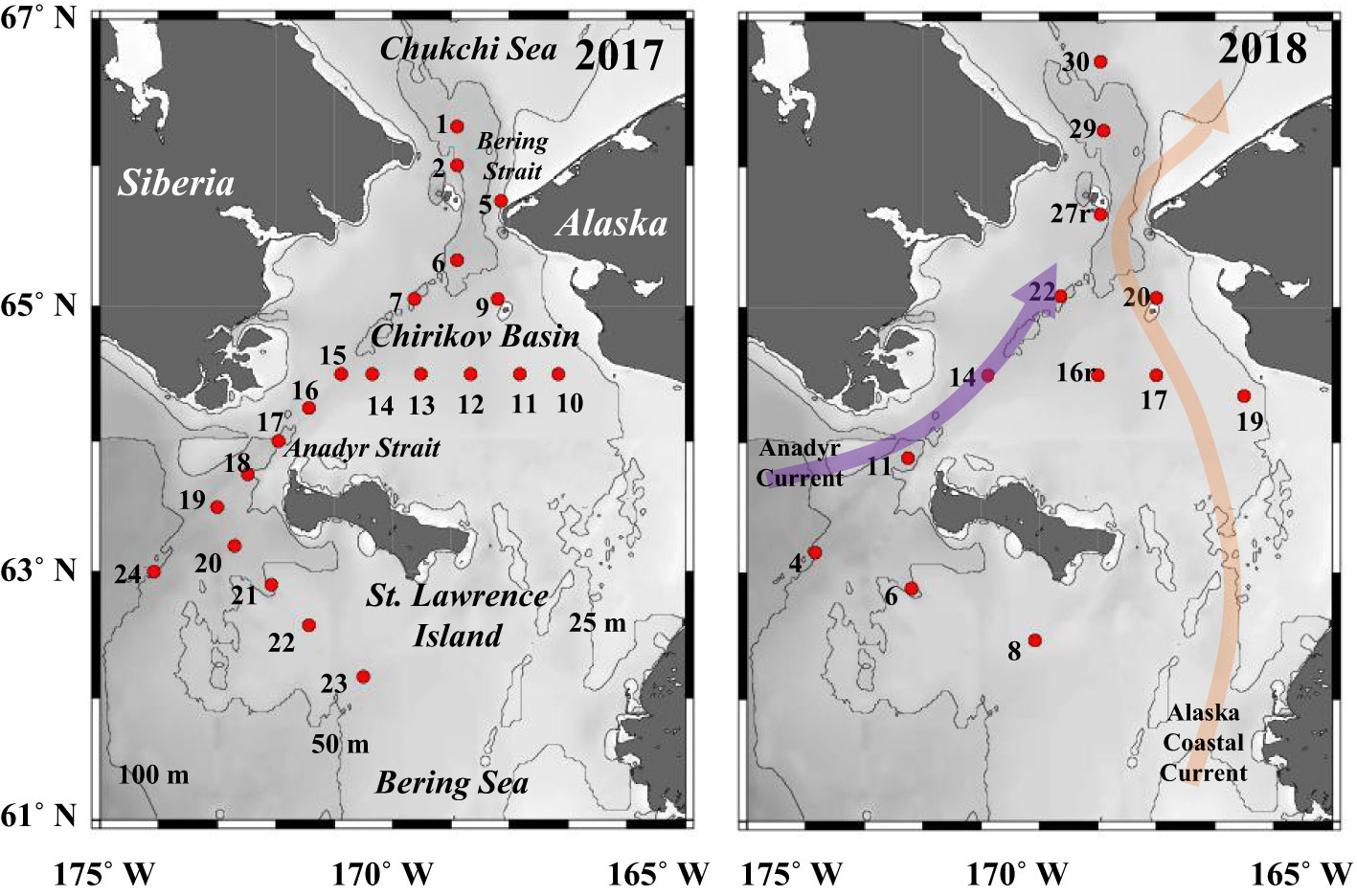
Figure 1 Location of stations in the northern Bering Sea during 11–22 July 2017and 2–12 July 2018. The numbers indicate station ID. Color arrows indicate main currents in this region.

2.3 Sample analysis

A total of 34 zooplankton samples were divided into 1/16–64 sections using a Motoda splitter (Motoda, 1959) and image data were obtained using ZooScan (Hydrooptic Inc.). First, the ZooScan scanning cell was filled with deionized water to scan the background image using VueScan (Version 9.5.24), and the divided zooplankton samples were then poured into the cell and scanned using VueScan. The scans of the samples were digitized using a minute function at 2400 dpi, where one pixel corresponded to 10.6 μm. Image data were semi-automatically separated per object using ZooProcess (Version 7.23) in Image J software (Version 1.410). All images scanned through ZooScan were uploaded onto the website Ecotaxa, where the gene level was semi-automatically identified based on datasets made from five manually identified samples per sampling year. All the images were manually checked to ensure that they had been correctly identified. Copepods were identified up to the genus level, and all other species were identified at the taxonomic level (from Order to Phylum). Images that could not be identified were classified as “unidentified organisms,” and those containing more than one object were classified as “multiple.” Images identified as “multiple” and “detritus” were excluded from further analysis. Copepods were divided into three groups: Calanus spp., Other large copepods (Eucalanus spp., Metridia spp., and Neocalanus spp.), and small copepods (Acartia spp., Centropages spp., Microcalanus spp., Microsetella spp., Oithona spp., Oncaea spp., Pseudocalanus spp., and Copepoda nauplii).

The size of each zooplankton was measured based on the study of Vandromme et al. (2012), using the ellipse major axis (L major, μm) and minor axis length (L minor, μm), which best fit the zooplankton image shape, and the volume of the ellipse (volume, mm³) and an equivalent spherical diameter (ESD, μm) with the same volume as the ellipse were identified using the following respective equations,

The biovolume (B: mm³ m^-2) was calculated using the filtered water volume (F: m^-3) calculated by using data of flowmeter, the tow distance (L), split ratio (s) and the elliptical volume (Volume, mm³) via the following equation.

2.4 Data analysis

Based on vertical profiles in temperature and salinity, thickness of water mass (according to Danielson et al., 2020) was calculated at each station.

Zooplankton biovolumes (mm³ m^-2) of 34 stations were used to conduct a cluster analysis, and they were transformed into fourth roots (∜X) to reduce the bias of abundant species. The similarities between the samples were examined using the Bray-Curtis similarity index. Dendrograms were created using the mean linkage method (unweighted pair group method using arithmetic means) and were classified into multiple groups by separating them at specific similarity levels (Field et al., 1982). Accompanying this analysis, similarity profile analysis (SIMPROF) was added to determine if groupings of the stations were statistically significant (at 5% significance level).The relationship between each sample and normalized hydrographic data (water temperature, salinity, chlorophyll-a fluorescence, MD, TSM and thickness in water masses) was evaluated using DistLM (distance based linear modeling) and a redundancy analysis (RDA). The parameters were selected by procedures consisting of Step-wise, r² and 999 permutations were used. The cluster analysis, DistLM, and RDA were conducted using the Primer 7 software (PRIMER-E Ltd., Albany, Auckland, New Zealand).

Differences in hydrographic (water temperature, salinity, chlorophyll-a fluorescence, and MD) and zooplankton size spectra parameters among the groups (identified by the cluster analysis based on zooplankton biovolume) were tested using the max-t method with a heteroscedastic consistent covariance estimation (HC3) (Herberich et al., 2010). The tests were conducted using R software with the packages “multcomp” and “sandwich” (version 4.1.2, R Core Team, 2021).

The NBSS analysis was conducted based on the size composition data obtained from ZooScan. Size data were used later analysis in the 300–3400 μm ESD range. Zooplankton larger than 3400 μm ESD (i.e., Cnidaria) were excluded from the analysis because they were not quantitatively sampled by net and were easily underestimated in ZooScan (Naito et al., 2019). Three ranges were set to categorize the sizes of zooplankton: small size (ESD 267–1024 μm), medium size (ESD 1024–2673 μm), and large size (ESD 2673–5759 μm). The NBSS X-axis is a log10 transformation of the biovolume for every log10 (0.25) ESD, (X: log10 zooplankton biovolume, [mm³ ind.^-1]) and the Y-axis is the log10 transformation of the integrated biovolume of the size classes classified by 100 μm ESD divided by the biovolume difference between adjacent size classes (Δbiovolume [mm³]) (Y: log10 zooplankton biovolume [mm³ m^-3]/Δbiovolume [mm³]). From X and Y, the linear equation of the NBSS is defined as Y = aX + b. Comparing the NBSS between the clustered groups, ANCOVA was performed using StatView, with the NBSS slope (a) applied as a response variable and intercept and (b) cluster groups applied as explanatory variables.

Zooplankton biomass and production were determined using ZooScan image data. First, the individual dry weight (DWind: mg DW ind^-1) was calculated from the biovolume per individual (mm³ ind.^-1), assuming that the density was equivalent to water (mm³ = mg), and the result was multiplied by the water content for each taxon (cf. Omori, 1969; Kiørboe, 2013; Nakamura et al., 2017; Matsuno unpublished data). The biomass per taxon was calculated using the following equation,

where s is the split ratio, F is the volume of filtered water (m³), and L is the towing distance (m). To estimate production (mg C m^-2 day^-1), the respiration rate (R: μL O₂ ind.^-1 h^-1) was calculated using the following equation (cf. Ikeda, 1985),

where DWind is the dry weight per individual, and T is the integrated mean water temperature at the sampling station. From the respiration rate, the production per individual, Pind (μg C ind^-1 day ²) was estimated using the following equation (cf. Ikeda and Motoda, 1978),

To calculate production (mg C m^-2 day^-1), Pind was summed for each taxon, divided by the volume of filtered water (m³), and then multiplied by the towing depth.

3 Results

3.1 Hydrography

In both years, there were similar variations in water temperature and salinity from east to west and with cold saline waters distributed on the western side (cf. Figure 2 and 3 in Kimura et al., 2022). On the other hand, water mass distributions were slightly different between the years (Figure 2). Warm Shelf Water (wSW) covered at surface layer in both years, and cold Shelf Water (cSW) and Anadyr Water (AnW) occupied below the water mass. However, Modified Winter Water (MWW) and Winter Water (WW) were only observed in the south of the St. Lawrence Island during 2017. Chlorophyll a fluorescence was higher in the Bering Strait during both years (cf. Figure 2 and 3 in Kimura et al., 2022). The MD occurred from March 23 to April 29 in 2018, which was earlier than in 2017 (April 4 to May 11) (cf. Figure 2 and 3 in Kimura et al., 2022).

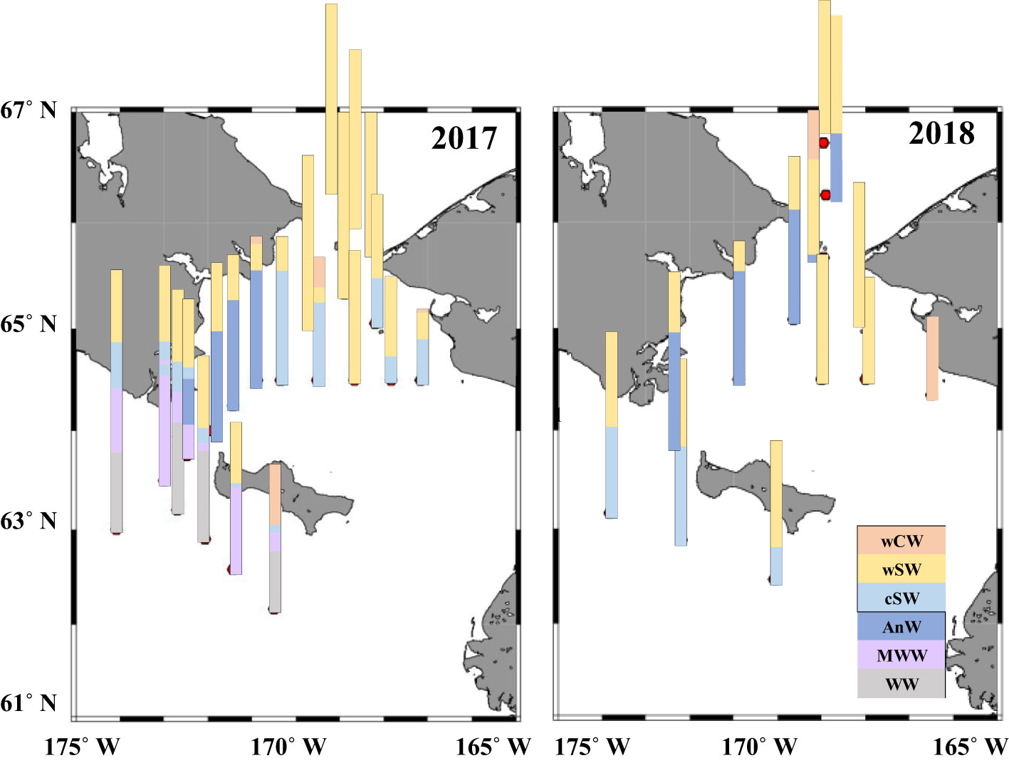
Figure 2 Spatial distribution of water masses in the northern Bering Sea during 11–22 July 2017 and 2–12 July 2018. Definition of water mass is according to Danielson et al. (2020). wCW, warm Coastal Water; wSW, warm Shelf Water; cSW, cool Shelf Water; AnW, Anadyr Water; MWW, Modified Winter Water; WW, Winter Water.

3.2 Zooplankton community

Cluster analysis based on the biovolumes of all zooplankton taxa revealed three groups (Y2017N, Y2017S, Y2018) with similarities of 62% and 65% (Figure 3A). By plotting the groups on a geological map, their spatial and interannual distributions were separated (Figure 3B). Y2017N was found from the Bering Strait to the Chirikov Basin in 2017 (Figure 3B); Y2017S was distributed along the Alaskan coast and southwest of St. Lawrence Island during both years; and Y2018 was spread widely from the Bering Strait to the southwest of St. Lawrence Island in 2018. Y2017N was dominated by Calanus spp. and other large copepods in similar proportions (Figure 3C); Y2017S (with the highest observed biovolume) was dominated by Calanus spp. and characterized by the contribution of Euphausiacea, small copepods, and Chaetognatha; and Y2018 contained the lowest biovolume but was dominated by small copepods and other large copepods. Each group was separately distributed in the RDA (Figure 4). Comparing hydrographic data among the groups, only salinity exhibited significant difference; higher value was seen in the Y2017N (32.3) than in the Y2018 (31.9) (Table 1).

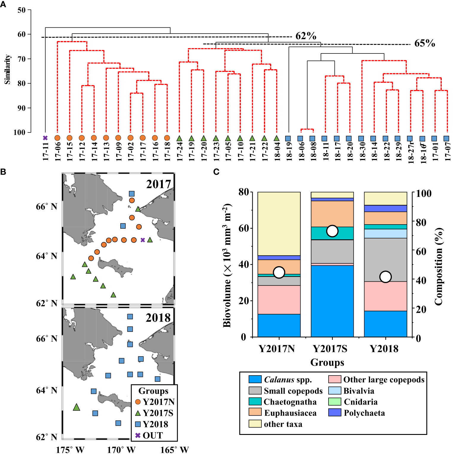
Figure 3 (A) Results of cluster analysis based on mesozooplankton biovolume using Bray–Curtis similarity connected with UPGMA in the northern Bering Sea during July 2017 and 2018. Three groups (Y2017N, Y2017S, Y2018) were identified with a similarity of 62% and 65% (dashed lines). The samples were named using the year and station ID. (B) Horizontal distribution of the three groups in the northern Bering Sea during July 2017 and 2018 identified by cluster analysis (cf. A). (C) Total biovolume and composition of each group.

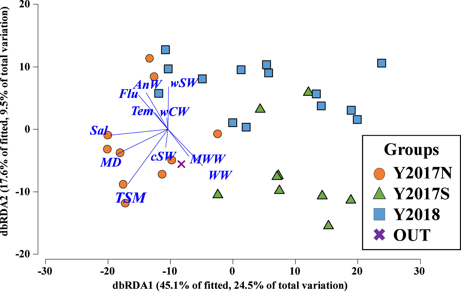
Figure 4 dbRDA plot of the three groups with environmental parameters. The direction of the lines indicate the relationship between environmental parameters and groups identified by cluster analysis (cf. Figure 3A) in the northern Bering Sea during July in 2017 and in 2018. Tem, water-column integrated mean temperature; Sal, water-column integrated mean salinity; Flu, water-column integrated fluorescence; MD, melt day; TSM, time since melt day to field sampling; wCW, warm Coastal Water; wSW, warm Shelf Water; cSW, cool Shelf Water; AnW, Anadyr Water; MWW, Modified Winter Water; WW, Winter Water.

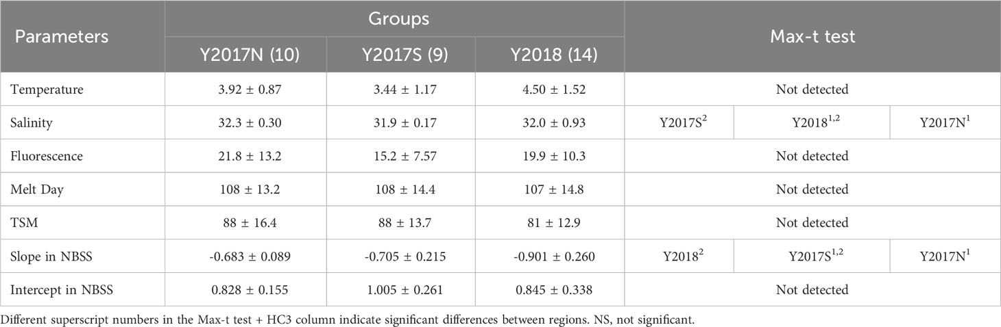
Table 1 Inter-group comparison of hydrographic and zooplankton size spectra parameters in the northern Bering Sea during July in 2017 and in 2018.

An NBSS analysis based on size composition was performed for the three groups classified by the cluster analysis. The results showed that the slope of Y2018 was significantly steeper (-0.8241) than that of Y2017N (-0.6843) (Figure 5, Table 1). Intercepts in NBSS were not different among the group significantly (Table 1). Biovolumes were summarized by 0.25 on the log10 axis and compared to NBSS plots, which clearly showed the contribution of each taxon to size classes (Figure 6). For all taxa, ESD 311–771 μm (-1.75–0 in log10 (mm³ ind.^-1)) with small copepods dominated, but Calanus spp. showed a high contribution at an ESD range of 1132–2439 μm (0–1 in log10 (mm³ ind.^-1)). In Y2018, with the significantly steeper NBSS slope), Bivalvia highly contributed to the size class of ESD 300–311 μm (-2 to -1.75, log10 (mm³ ind.^-1)) (Figure 6). other large copepods were dominant in the larger size classes of groups A and C, whereas Chaetognatha was dominant in the same size class of Y2017S. Euphausiacea was particularly abundant in the middle size class of groups Y2017N and Y2018.

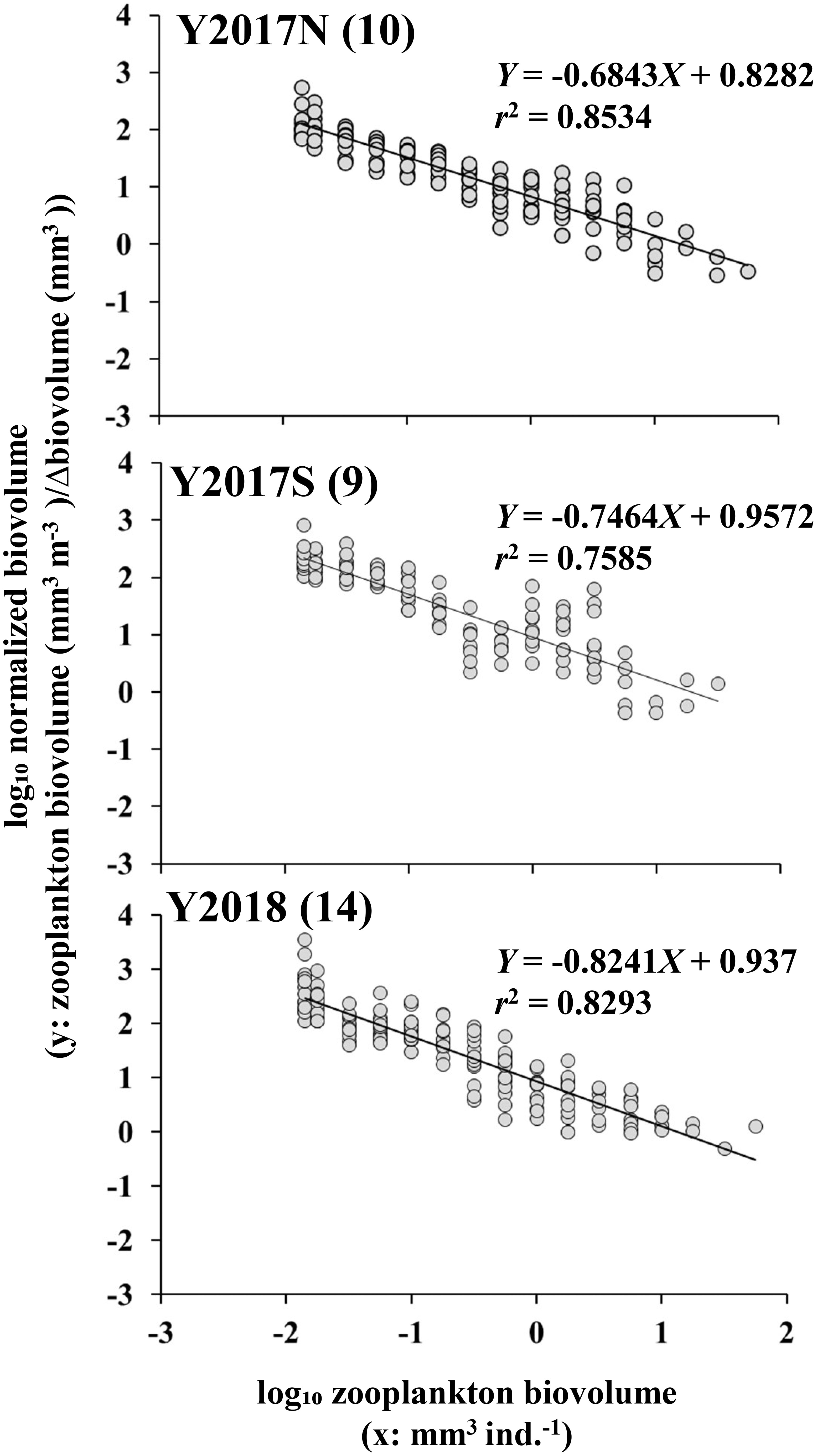
Figure 5 NBSS of three groups identified from cluster analysis of mesozooplankton biovolume (cf. Figure 3A) in the northern Bering Sea during July 2017 and 2018. Numbers in parenthesis indicate the number of stations belonging to each group.

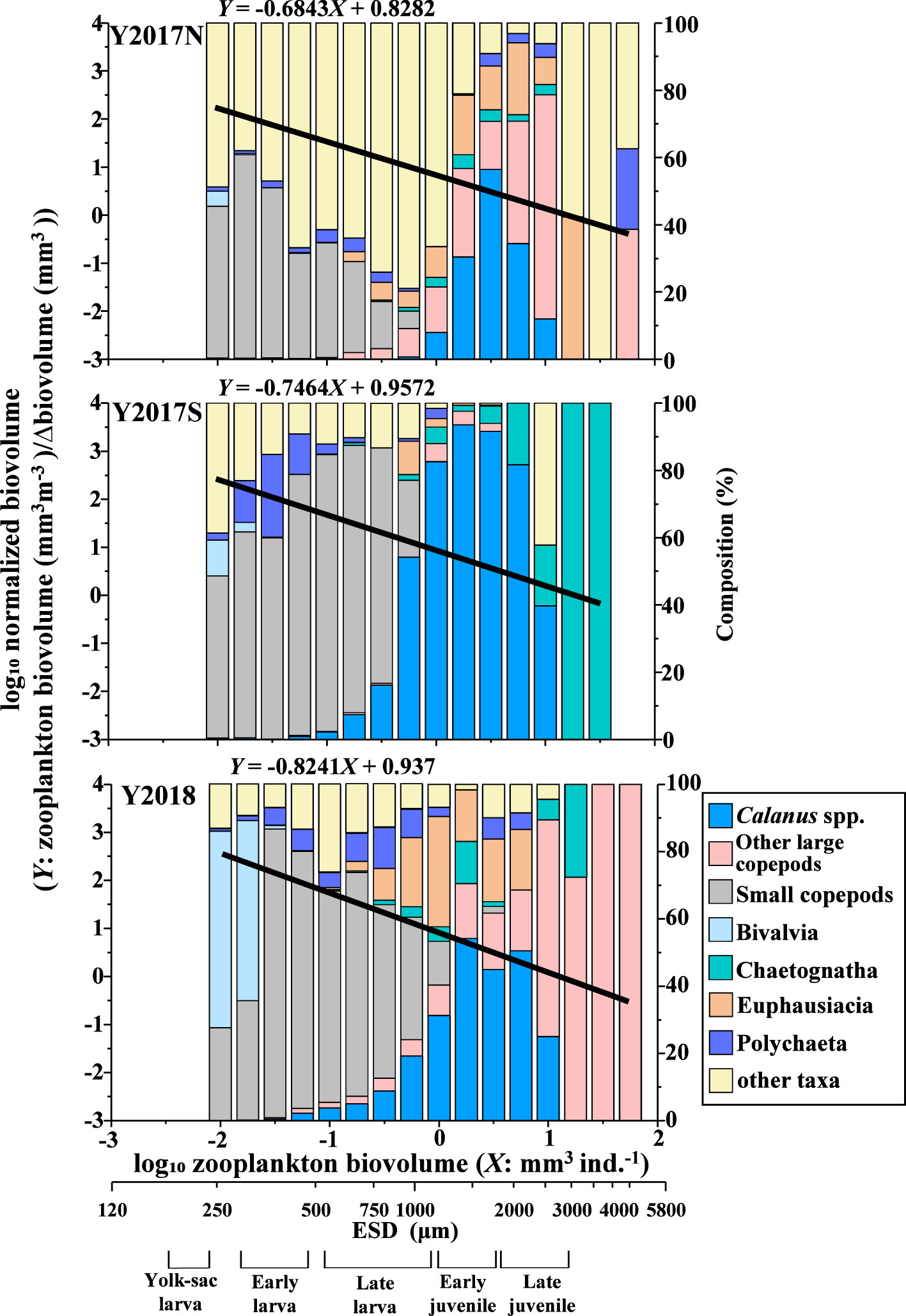
Figure 6 Species composition and biovolume within the interval of 0.25 in log10, and the NBSS line of the three groups identified from conducting a cluster analysis of mesozooplankton biovolume (cf. Figure 3C) in the northern Bering Sea during July 2017 and 2018. The species composition was calculated by summarizing the biovolume for all specimens in each size class. Prey size range for each stage of fish are shown at the bottom horizontal axis (cf. Jacobsen et al., 2020).

A comparison between the size range and the available prey for fish (Pacific cod) (cf. Jacobsen et al., 2020) revealed no yolk-sac larvae specimens in the predator size classes (Figure 6). In Y2017N, other large copepods and Euphausiacea dominated the late larval and early juvenile stage predator size class; in Y2017S, large Calanus spp. dominated the late larvae to early juveniles predator size class but Chaetognatha was dominant in the late juvenile stage; and in Y2018, small copepods were dominant in the late larval stage predator size class.

Biomass ranged from 4.60–11.49 g DW m^-2 and was the highest and lowest in Y2017S and Y2017N, respectively (Figure 7A, Supplementary Table 1). Y2017N was characterized by a high proportion of Calanus spp., other large copepods, and Euphausiacea (Figure 7A). Y2017S, which had the highest biomass among the three groups, was dominated by Calanus spp. In Y2018, small copepods dominated, followed by Calanus spp. and other large copepods (Figure 7A), and the proportion of Bivalvia was higher (9.14%) than that of the other groups (0.05–0.2%). Production ranged from 52.6–119 mg C m^-2 day^-1 in the three groups, with the highest in Y2017S and the lowest in Y2017N (Figure 7B; Supplementary Table 2). Y2017N, which showed the lowest production rates, showed a high contribution from Calanus spp., other large copepods, and Euphausiacea. Production was dominated by copepods in Y2017S (66%), whereas small copepods supported the production of Y2018, which was also characterized by the production of Bivalvia. Euphausiacea showed the second highest production following copepods in all three groups, ranging from 6.68–13.93 mg C m^-2.

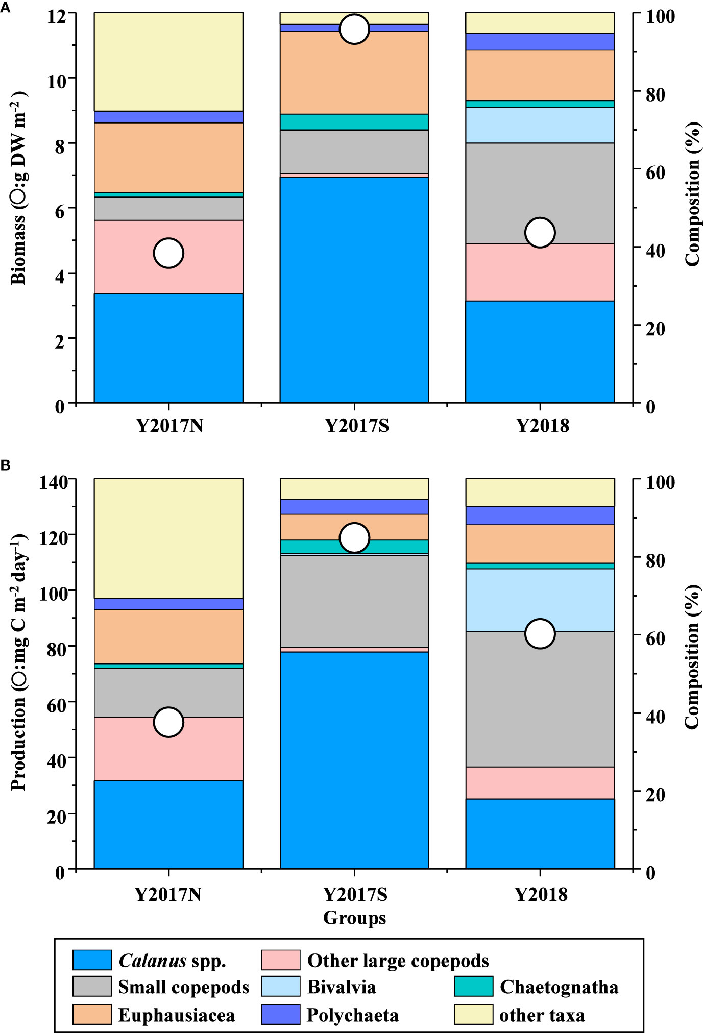
Figure 7 (A) Species composition and mean biomass and (B) production in each group as identified from conducting a cluster analysis of mesozooplankton biovolume (cf. Figure 3A) in the northern Bering Sea during July 2017 and 2018.

4 Discussion

4.1 Limitation of ZooScan

It is not always possible to classify small objects (especially below 200 µm ESD) via image analysis with ZooScan, as it has a pixel resolution of 10.6 µm (Gorsky et al., 2010). Many studies using ZooScan have focused on > 300 µm ESD zooplankton (i.e., Colas et al., 2017), and we therefore also only analyzed this size range. The parameters of abundance and biovolume accuracy obtained using ZooScan are largely consistent with the microscopic counts and size measurements of copepods (Gorsky et al., 2010; Garcia-Comas et al., 2011; Cornils et al., 2022), and significant regression is present for ESD 1–6 mm-sized copepods, in particular (Forest et al., 2012). However, abundance and biomass based on ZooScans of Chaetognatha, Appendicularia, and Cnidaria are likely to be underestimated because it is difficult to analyze transparent objects using ZooScan and there is large variability in the organic matter content of gelatinous zooplankton (Lehette and Hernandez-Leon, 2009; Naito et al., 2019; Cornils et al., 2022). Also, they are not efficiently caught by nets. Therefore, a considerable amount of attention to detail is required when analyzing such taxa with ZooScan.

4.2 NBSS analysis

The slope and intercept of the NBSS explain the zooplankton size composition characteristics: the NBSS intercept is reflected by zooplankton standing stock and primary production, whereas the slope is reflected by productivity and trophic levels (Zhou, 2006). In a typical marine ecosystem, the NBSS slope approaches -1 (Platt and Denman, 1977; Kerr and Dickie, 2001). In this study, all slopes were less than -1: this indicated that larger objects were dominant, which is commonly observed after phytoplankton blooms (Vandromme et al., 2014). NBSS slopes can be easily altered by top-down and bottom-up effects within an ecosystem (Suthers et al., 2006). In the top-down case, the slope of the NBSS becomes steeper as middle-to large-sized plankton decrease with predation by mammals and fishes. Therefore, a negative relationship is assumed between predator abundance and slope (Suthers et al., 2006). In a bottom-up effect, the slope becomes steeper as primary production increases, consequently increasing the size of small zooplankton (Moore and Suthers, 2006). When discussing top-down and bottom-up effects, it is important to clarify the actual prey-predator relationship (Yurista et al., 2014). As a result, an increasing number of reports have combined NBSS analysis with ZooScan to reveal taxonomic information (i.e., Cornils et al., 2022).

4.3 Characteristics of clustering groups

A cluster analysis based on the biovolume was used to reveal regional and interannual changes in zooplankton communities (Matsuno et al., 2012). The distribution and composition showed similar tendencies to those of microscopic analyses (cf. Figure 4 and 5 in Kimura et al., 2022), which suggests that identification at the taxon level (genus level for copepods) using the ZooScan approach can be used to detect trends at a level similar to that detected via microscopic analysis.

In northern Bering Sea, zooplankton community changes under the influence of water masses (Kimura et al., 2020). The water masses changes seasonally (Danielson et al., 2020), so it is well reported that zooplankton communities are different between months. However, since there is no report about difference between shorter time scale, such as week. Thus, in this study, sampling time between two years differ only 11 days, which potentially influences zooplankton community, but quantitative evaluation (or back calculation) is not possible due to the lack of information.

Y2017N was observed in 2017 from the Bering Strait to the Chirikov Basin, and it corresponds to the Y2017N presented in our previous study (Kimura et al., 2022). This group was characterized by low abundance (Table 2 in Kimura et al., 2022) and biomass, and small copepods dominated the small size classes. The group showed higher salinity than the other group, which means AnW mainly occupied with water column at the station observed Y2017N. The middle class of this group was dominated by other large copepods and Euphausiacea transported from Anadyr Bay (Springer et al., 1989; Ashjian et al., 2010; Moore et al., 2010). Euphausiacea dominated 60%–90% of the stomach contents of cetaceans in the study area; they are considered to play an important role in the food web but are not likely to establish expatriates in the present state (Moore et al., 2010). In Euphausiacea, Thysanoessa inermis, T. raschii, Meganyctiphanes norvegica are carnivorous, which can limit the abundance of Calanus spp. (Bamstedt and Karlson, 1998). The occurrence of other large copepods (composed of Eucalanus spp., Metridia spp., and Neocalanus spp.) was consistent with the characteristics of a community found during the summer in a previous study (Eisner et al., 2013). In the Chirikov Basin, the zooplankton community structure showed monthly changes accompanying surface water mass changes from June to September (Kimura et al., 2020). During June and July, other large copepods and Euphausiacea were abundant due to the inflow of AnW, Calanus spp., and Euphausiacea. In contrast, in August, the number of Bivalvia larvae, barnacle larvae, and Appendicularia increased significantly. The community was then dominated by Calanus nauplii and other small copepods (Centropages spp. and Cyclopoida) (Kimura et al., 2020). The NBSS slope of Y2017N is gentle due to the dominance of Calanus spp., other large copepods, and Euphausiacea in the middle- and large-size classes, and it has been suggested that the slope of the NBSS will become steeper with an increase in benthic larvae (Matsuno et al., 2012; Kimura et al., 2020).

The NBSS slopes of Y2017N and Y2017S (seen south of St. Lawrence Island) were similar, but their compositions differed: Calanus spp. were dominant in the middle-sized class in Y2017S, but not in Y2017N. South of St. Lawrence Island, winter water is distributed in the lower layers where Calanus glacialis is abundant (Pinchuk and Eisner, 2017). It is also known that in cold years (late sea-ice retreat), the abundance of large copepods (C. glacialis) increases while that of small copepods and Cnidaria decreases (Ershova et al., 2015). In 2017, late sea ice melt (compared to 2018) induced ice-edge blooms in late April (Kikuchi et al., 2020); therefore, large copepods had grown to the C5 stage by July when our survey was conducted (Kimura et al., 2022). In other words, Y2017S, as seen in this study, is the community generally found south of St. Lawrence Island during the summer of cold years. According to the results of the size analysis, the zooplankton abundance in the middle-sized class was low, and the large-sized class was dominated by Chaetognatha. Chaetognatha is a typical copepod predator (Feigenbaum, 1982; Kimmel et al., 2006); it is therefore likely that it fed on middle-sized copepods in Y2017S, which resulted in their decreased abundance. This suggests that the food chain was functional in Y2017S.

The small size glass of Y2018 (which produced the steepest NBSS slope) was dominated by Bivalvia larvae, and this is consistent with the large seasonal occurrence of Bivalvia larvae observed in the study area (Moore et al., 2003; Moore et al., 2006). Changes in the slope of the NBSS due to the dominance of small copepods have also been reported in the Chukchi Sea (Matsuno et al., 2012) and Atlantic sector of the Arctic Ocean (Basedow et al., 2010). As Bivalvia larvae typically settle 2–6 weeks after emergence (Steidinger and Walker, 1984), the steep slope of the NBSS in Y2018 does not indicate high productivity, but it rather indicates the seasonal recruitment of meroplankton.

4.4 Impact of early sea-ice melt on higher trophic levels

Sea ice melted from April to May in 2017, resulting in an ice-edge bloom and early copepod reproduction that induced a high abundance of large (late stage) copepods during summer (Kimura et al., 2022). However, sea ice melted earlier (from March to April) in 2018; therefore, an ice-edge bloom did not occur, and an open-water bloom occurred instead (Kikuchi et al., 2020). The reproduction of copepods was delayed in relation to the late open-water bloom, which resulted in a decreased abundance of large copepods during summer (Duffy-Anderson et al., 2019; Kimura et al., 2022). In this study, the results of the ZooScan analysis showed clear annual variations, with groups Y2017N and Y2017S dominating in 2017 and Y2018 dominating in 2018.

Y2017S, observed in 2017, exhibited the highest biomass. Calanus spp. largely contributed to this group, and this was attributed to late sea ice melting in cold years, as mentioned above (Ershova et al., 2015; Kimura et al., 2022). A high abundance of benthic larvae (Grebmeier et al., 2006) and a high biomass of copepods have been observed South of St. Lawrence Island (Kimura et al., 2022). According to the NBSS results, Y2017S was the most productive community with a functioning food chain among the three groups. This result means that the south of St. Lawrence Island is not only an important area for maintaining the zooplankton population, but also for efficiently transferring production to higher trophic levels.

Y2018 had the lowest biovolume, and this group corresponded to group D reported by Kimura et al. (2022). The biomass of Y2018 in this study was similar to that of Y2017N. However, production was higher than that of Y2017N because of the high production of small copepods. Large copepods in the study area are efficient prey for higher trophic levels, as they store rich lipids in their body (Lee, 1974), whereas small copepods rarely store lipids because of their low nutrient content (Norrbin et al., 1990). The small copepods in this study contained minimal amounts of lipids (Kimura et al., 2022). This group was also characterized by the dominance of Bivalvia larvae in the small class due to the seasonal reproduction of meroplankton. The carbon content of Bivalvia larva was 1.4–1.5%, which was much lower than that of copepods (Viverberg and Frank, 1976; Steidinger and Walker, 1984) and indicated that the food quality was too low for higher trophic levels. Lowering the nutrients and fats of prey decreases the winter survival rate of fish such as salmon or Arctic cod (Heintz et al., 2013). Therefore, it is suggested that in Y2018, the production of low fat meroplankton and small zooplankton was not transferred sufficiently to higher trophic levels, which might have affected their abundance (Springer et al., 1989; Huntington et al., 2020).

Fish generally exhibit grazing selectivity (for example, O’Brien, 1979). It is difficult for fish to detect small prey (and they contain low levels of nutrients); therefore, they tend to prey on larger foods (O’Brien, 1979). Walleye pollack (Theragra chalcogramma) is an abundant species in the study area and it preys on small copepods when they dominate in warm years, whereas it prays on large copepods and Euphausiacea when they dominate in cold years. This is likely because they graze on larger species during summer to efficiently store lipids for overwintering (Coyle et al., 2011; Heintz et al., 2013). Therefore, the prey-size composition provides important information about the survival rate of fish. To compare the growth stage of the fish larvae with the prey size, we determined the available prey size range for each growth stage. In this study, the available prey size for yolk-sac larvae was not detected, possibly because ZooScan could not analyze copepod eggs, which are the main food source for yolk-sac larvae. From late larvae to early juveniles, the most important period for survival (Jacobsen et al., 2020), the available food differed across the groups. Fat-rich other large copepods and Euphausiaceae with rich fats were relatively abundant in Y2017N and Y2018; however, their biovolumes were low. Therefore, because the rate at which fish encountered these foods was low and they experienced low food availability. When fish do not receive sufficient energy, their populations and survival rates are affected (Springer et al., 1989; Heintz et al., 2013; Huntington et al., 2020). In contrast, large and fat-rich Calanus spp. was found to be abundant in Y2017S, which suggested that it was readily available to fish. In addition, sufficient Chaetognatha populations for fish were seen in Y2017S; therefore, production by small and large copepods was efficiently transferred to fish in Y2017S.

In conclusion, the zooplankton community and size compositions in the northern Bering Sea differed between 2018 (an early sea ice melt year) and 2017 (a normal sea ice melt year). In 2017, Y2017N (dominated by other large copepods and Euphausiacea) was observed in the Chirikov Basin and was influenced by ACW, whereas Y2017S (dominated by Calanus spp. and Chaetognatha) was distributed to the south of St. Lawrence Island. In 2018, however, Y2017S was observed in the same area as that in 2017, and Y2018 (dominated by small copepods and Bivalvia) was distributed widely in the northern Bering Sea. The NBSS analysis showed that the slopes of groups Y2017N and Y2017S were similar; however, the species composition differed between the groups. Y2017N was dominated by medium- or large-sized plankton (other large copepods and Euphausiacea) transported from Anadyr Bay. In contrast, the middle-sized class of Y2017S was dominated by Calanus spp., which is consistent with the community observed during summer in cold years. The abundance of the middle-sized class in this group was low, and this may have been due to Chaetognatha grazing on middle-sized copepod classes. The NBSS slope of Y2018 was the steepest in relation to the seasonal occurrence of Bivalvia larvae. In 2018, secondary production in the study area increased due to the increased abundance of small copepods, and production was contributed to by small copepods and Bivalvia larvae. As these small zooplankton are considered low-nutritional prey, the number of higher trophic levels may have decreased.

Data availability statement

The original contributions presented in the study are included in the article/Supplementary Material. Further inquiries can be directed to the corresponding author.

Ethics statement

The manuscript presents research on animals that do not require ethical approval for their study.

Author contributions

KM and AY designed the study; AY performed field sampling; SK analyzed the samples; SK and KM analyzed the data; and SK and KM wrote the paper with contributions from all authors. All authors contributed to the article and approved the submitted version.

Funding

The author(s) declare financial support was received for the research, authorship, and/or publication of this article. This study was funded by the Arctic Challenge for Sustainability (ArCS) (Program Grant Number JPMXD1300000000) and the Arctic Challenge for Sustainability II (ArCS II) (Program Grant Number JPMXD1420318865) projects. This work was also supported by the Environment Research and Technology Development Fund (JPMEERF20214002) of the Environmental Restoration and Conservation Agency of Japan. Furthermore, this work was partially supported by the Japan Society for the Promotion of Science (JSPS) KAKENHI, Grant Numbers JP21H02263 (B), JP20K20573 (Pioneering), JP20H03054 (B), JP20J20410 (B), JP19H03037 (B), JP18K14506 (Early Career Scientists), and JP17H01483 (A).

Acknowledgments

We thank the captain, officers, crew, and researchers onboard the T/S Oshoro-Maru (Hokkaido University) for their crucial contributions to field sampling. The archived ADS dataset was provided by the Arctic Data archive System (ADS) developed by the National Institute of Polar Research.

Conflict of interest

The authors declare that the research was conducted in the absence of any commercial or financial relationships that could be construed as a potential conflict of interest.

Publisher’s note

All claims expressed in this article are solely those of the authors and do not necessarily represent those of their affiliated organizations, or those of the publisher, the editors and the reviewers. Any product that may be evaluated in this article, or claim that may be made by its manufacturer, is not guaranteed or endorsed by the publisher.

Supplementary material

The Supplementary Material for this article can be found online at: https://www.frontiersin.org/articles/10.3389/fmars.2023.1233492/full#supplementary-material

References

Ashjian C. J., Braund S. R., Campbell R. G., George J. C. C., Kruse J., Maslowski W., et al. (2010). Climate variability, oceanography, bowhead whale distribution, and iñupiat subsistence whaling near barrow, Alaska. arctic institute North America 63, 179–194. doi: 10.14430/arctic973
Bamstedt U., Karlson K. (1998). Euphausiid predation on copepods in coastal waters of the Northeast Atlantic. Mar. Ecol. Prog. Ser. 172, 149–168. doi: 10.3354/meps172149
Barid M. E., Timko P. G., Middleton T. J., Cox D. R., Suthers I. M. (2008). Biological properties across the Tasman Front off southeast Australia. Deep Sea Res. 55, 1438–2455.
Basedow S. L., Tande K. S., Zhou M. (2010). Biovolume spectrum theories applied: spatial patterns of trophic levels within a mesozooplankton community at the polar front. J. Plankton Res. 32, 1105–1119. doi: 10.1093/plankt/fbp110
Basyuk E., Zuenko Y. (2020). Extreme oceanographic conditions in the northwestern Bering Sea in 2017–2018. Deep-Sea Res. II 181–182, 104909. doi: 10.1016/j.dsr2.2020.104909
Coachman L. K., Aagaard K., Tripp E. B. (1975). Bering Strait the Regional Physical Oceanography Vol. 172 (Seattle, Washington: University of Washington Press).
Colas F., Tardivela M., Perchocb J., Lunvenb M., Foresta B., Guyaderc G., et al. (2017). The ZooCAM, a new in-flow imaging system for fast onboard counting, sizing and classification of fish eggs and metazooplankton. Prog. Oceanogr. 166, 54–65. doi: 10.1016/j.pocean.2017.10.014
Cornils A., Thomisch K., Hase J., Hildebrandt N., Auel H., Niehoff B. (2022). Testing the usefulness of optical data for long-term monitoring of zooplankton: taxonomic composition, abundance, biomass, and size spectra from ZooScan image analysis. Limnol. Oceanogr-Meth. 20, 428–450. doi: 10.1002/lom3.10495
Cornwall W. (2019). Vanishing Bering Sea ice poses a climate puzzle. Science 364, 616–617. doi: 10.1126/science.364.6441.616
Coyle K. O., Eisner L. B., Mueter F. J., Pinchuk A. I., Janout M. A., Cieciel K. D., et al. (2011). Climate change in the southeastern Bering Sea: impacts on pollock stocks and implications for the oscillating control hypothesis. Fish. Oceanogr. 20, 139–156. doi: 10.1111/j.1365-2419.2011.00574.x
Danielson S. L., Ahkinga O., Ashjian C., Basyuk E., Cooper L. W., Eisner L., et al. (2020). Manifestation and consequences of warming and altered heat fluxes over the Bering and Chukchi Sea continental shelves. Deep. Sea. Res. II. 177, 104781. doi: 10.1016/j.dsr2.2020.104781
Duffy-Anderson J. T., Stabeno P., Andrews A. G. III, Cieciel K., Deary A., Farley E., et al. (2019). Responses of the northern Bering Sea and southeastern Bering Sea pelagic ecosystems following record-breaking low winter sea ice. Geophys. Res. Lett. 46, 9833–9842. doi: 10.1029/2019GL083396
Eisner L., Hillgruber N., Martinson E., Maselko J. (2013). Pelagic fish and zooplankton species assemblages in relation to water mass characteristics in the northern Bering and southeast Chukchi Seas. Polar Biol. 36, 87–113. doi: 10.1007/s00300-012-1241-0
Ershova E. A., Hopcroft R. R., Kosobokova K. N. (2015). Inter-annual variability of summer mesozooplankton communities of the western Chukchi Sea: 2004–2012. Polar Biol. 38, 1461–1481. doi: 10.1007/s00300-015-1709-9
Feigenbaum D. (1982). Feeding by the chaetognath, Sagitta elegans, at low temperatures in Vineyard Sound, Massachusetts. Am. Soc. Limnology Oceanography 27, 699–6706. doi: 10.4319/lo.1982.27.4.0699
Field J. G., Clarke K. R., Warwick R. M. (1982). A practical strategy for analyzing multispecies distribution patterns. Mar. Ecol. 8, 37–52. doi: 10.3354/meps008037
Forest A., Stemmann L., Picheral M., Burdorf L., Robert D., Fortier L., et al. (2012). Size distribution of particles and zooplankton across the shelf basin system in southeast Beaufort Sea: combined results from an Underwater Vision Profiler and vertical net tows. Biogeoscience 9, 1301–1320. doi: 10.5194/bg-9-1301-2012
Garcia-Comas C., Stemmann L., Icanez F., Berline L., Mazzocchi M. G., Gasparini S., et al. (2011). Zooplankton long-term changes in the NW Mediterranean Sea: Decadal periodicity forced by winter hydrographic conditions related to large-scale atmospheric changes? J. Mar. Syst. 87, 216–226. doi: 10.1016/j.jmarsys.2011.04.003
Gorsky G., Ohman M. D., Picheral M., Gasparini S., Stemmann L., Romagnan J., et al. (2010). Digital zooplankton image analysis using the ZooScan integrated system. J. Plankton Res. 32, 285–303. doi: 10.1093/plankt/fbp124
Grebmaier J. M., Bluhm B. A., Cooper L. W., Danielson S. L., Arrigo K. R., Blanchard A. L., et al. (2015). Ecosystem characteristics and processes facilitating persistent macrobenthic biomass hotspots and associated benthivory in the Pacific Arctic. Prog. Oceanogr 136, 92–114. doi: 10.1016/j.pocean.2015.05.006
Grebmeier J. M., Cooper L. W., Feder H. M., Sirenko B. I. (2006). Ecosystem dynamics of the pacific-influenced northern Bering and Chukchi seas in the Amerasian Arctic. Prog. Oceanogr. 71, 331–361. doi: 10.1016/j.pocean.2006.10.001
Grosjean P., Picheral M., Warembourg C., Gorsky G. (2004). Enumeration, measurement, and identification of net zooplankton samples using the ZOOSCAN digital imaging system. ICES. J. Mar. Sci. 61, 518–525. doi: 10.1016/j.icesjms.2004.03.012
Heintz R. A., Siddon E. C., Farley J. E.V., Napp. J. (2013). Correlation between recruitment and fall condition of age-0 pollock (Theragra chalcogramma) from the eastern Bering Sea under varying climate conditions. Deep-Sea Res. II 94, 150–156. doi: 10.1016/j.dsr2.2013.04.006
Herberich E., Sikorski J., Hothorn T. (2010). A Robust procedure for comparing multiple means under heteroscedasticity in unbalanced designs. PLoS One 5, e9788. doi: 10.1371/journal.pone.0009788
Herman A. W., Harvey M. (2006). Application of normalized biomass size spectra to laser optical plankton counter net intercomparisons of zooplankton distributions. J. Geophy. Res. 111, C05S05.
Huntington H. P., Danielson S. L., Wiese F. K., Baker M., Boveng P., Citta J. J., et al. (2020). Evidence suggests potential transformation of the Pacific Arctic ecosystem is underway. Nat. Clim. Change 10, 342–348. doi: 10.1038/s41558-020-0695-2
Ikeda T. (1985). Metabolic rates of epipelagic marine zooplankton as a function of body mass and temperature. Mar. Biol. 85, 1–11. doi: 10.1007/BF00396409
Ikeda T., Motoda S. (1978). Zooplankton production in the Bering Sea calculated from 1957-1970 Oshoro-Maru data. Mar. Sci. Comms. 4, 329–346.
Jacobsen S., Nielsel K. K., Kristiansen R., Grønkjær P., Gaard E., Steingrund P. (2020). Diet and prey pregerences of larval and pelagic juvenile Faroe Plateau cod (Gadus morhua). Mar. Biol. 167, 122. doi: 10.1007/s00227-020-03727-5
Kikuchi G., Abe H., Hirawake T., Samhythm M. (2020). Distinctive spring phytoplankton bloom in the Bering Strait in 2018: A year of historically minimum sea ice extent. Deep-Sea Res. II 181–182, 104905. doi: 10.1016/j.dsr2.2020.104905
Kimmel D. G., Roman M. R., Zhang X. (2006). Limnol. Oceangr. 51, 131–141. doi: 10.4319/lo.2006.51.1.0131
Kimura F., Abe Y., Matsuno K., Hopcroft R. R., Yamaguchi A. (2020). Seasonal changes in the zooplankton community and population structure in the northern Bering Sea from June to September 2017. Deep-Sea Res. II 181–182, 104901. doi: 10.1016/j.dsr2.2020.104901
Kimura F., Matsuno K., Abe Y., Yamaguchi A. (2022). Effects of early sea-ice reduction on zooplankton and copper pod population structure in the northern Bering Sea during the summers of 2017 and 2018. Front. Mar. Sci. 9, 808910. doi: 10.3389/fmars.2022.808910
Kiørboe T. (2013). Zooplankton body composition. Limnol. Oceanogr. 58 (5), 1843–1850. doi: 10.4319/lo.2013.58.5.1843
Lehette P., Hernandez-Leon S. (2009). Zooplankton biomass estimation from digitized images: a comparison between subtropical and Antarctic organisms. Limnol. Oceanogr.: Methods 7, 304–308. doi: 10.4319/lom.2009.7.304
Matsuno K., Yamaguchi A., Imai I. (2012). Biomass size spectra of mesozooplankton in the Chukchi Sea during the summers of 1991/1992 and 2007/2008: and analysis using optical plankton counter data. ICES J. Mar. Sci. 69, 1205–1217.
Meeren T. D., Næss T. (1993). How does cod (Gadus morhua) cope with variability in feeding conditions during early larval stages? Mar. Biol. 116, 637–647. doi: 10.1007/bf00355482
Moore S. E., George J. C. C., Sheffield G., Bacon J., Ashjian C. J. (2010). Bowhead whale distribution and feeding near barrow, Alaska, in late summer 2005–06. Arctic Institute North America. 63, 195–205. doi: 10.14430/arctic974
Moore S. E., Grebmeier J. M., Davis J. R. (2003). Gray whale distribution relative to forage habitat in the northern Bering Sea: current conditions and retrospective summary. Can. J. Zool. 81, 734–742. doi: 10.1139/z03-043
Moore S. E., Stafford K. M., Mellinger D. K., Hildebrand J. A. (2006). Listen to large whales in the offshore waters of Alaska. Bioscience 56, 49–55. doi: 10.1139/z03-043
Moore S. K., Suthers I. M. (2006). Evaluation and correction of subresolved particles by the optical plankton counter in three Australian estuaries with pristine to highly modified catchments. J. Geophys. Res. 111, 148–227. doi: 10.1029/2005JC002920
Naito A., Abe Y., Matsuno K., Nishizawa B., Kanna N., Sugiyama S., et al. (2019). Surface zooplankton size and taxonomic composition in Bowdoin Fjord, north-western Greenland: a comparison of ZooScan, OPC, and microscopic analyses. Polar Sci. 19, 120–129. doi: 10.1016/j.polar.2019.01.001
Nakamura Y., Somiya R., Suzuki N., Hidaka-Umetsu M., Yamaguchi A., Lindsay D. J. (2017). Optics-based surveys of large unicellular zooplankton: a case study on radiolarians and paederines. Plankton Benthos Res. 12, 95–103. doi: 10.3800/pbr.12.95
Norrbin M. F., Olsen R. E., Tande K. S. (1990). Seasonal variation in lipid class and fatty acid composition of two small copepods in Balsqorden, northern Norway. Mar. Biol. 105, 205–211. doi: 10.1007/BF01344288
O’Brien W. J. (1979). The predator–prey interaction of planktivorous fish and zooplankton: Recent research with planktivorous fish and their zooplankton prey shows the evolutionary thrust and parry of the predator-prey relationship. Am. Sci. 67, 572–581.
Omori M. (1969). Weight and chemical composition of important oceanic zooplankton in the north Pacific Ocean. Mar. Biol. 3, 2–10. doi: 10.1007/BF00355587
Pinchuk A. I., Eisner L. B. (2017). Spatial heterogeneity in zooplankton summer distribution in the eastern Chukchi Sea in 2012–2013 as a result of large-scale interactions of water masses. Deep-Sea Res. II 1135, 27–39. doi: 10.1016/j.dsr2.2016.11.003
Platt T., Denman K. (1977). Organisation in the pelagic ecosystem. Helgoländer Wiss. Meeresunters 30, 575–581. doi: 10.1007/BF02207862
R Core Team. (2021). R: a language and environment for statistical computing (Vienna, Australia: R Foundation for Statistical Computing). Available at: https://www.R-project.org/.
Sheldon R. W., Sutcliffe J. W.H., Parajape M. A. (1977). Structure of pelagic food chain and relationship between plankton and fish production. J. Fish. Res 34, 2344–2353. doi: 10.1139/f77-314
Springer A. M., McRoy C. P., Turco K. R. (1989). The paradox of pelagic food webs in the northern Bering Sea – II Zooplankton communities. Cont. Shelf Res. 9, 359–386. doi: 10.1016/0278-4343(89)90039-3
Springer A. M., McRoy C. P., Turco K. R. (1993). The paradox of pelagic food webs in the northern Bering Sea-II. Zooplankton communities. Cont. Shelg Res. 9, 359–386. doi: 10.1016/0278-4343(89)90039-3
Sprules W. G., Munawar M., Jin E. H. (1988). Plankton community stducture and size spectra in the Georgian Bay and North Channel ecosystems. Hydrobiologia 163, 135–140. doi: 10.1007/BF00026925
Stabeno P. J., Bell S. W. (2019). Extreme conditions in the Bering Sea, (2017–2018): record-breaking low sea-ice extent. Geophys. Res. Lett. 46, 8952–8959. doi: 10.1029/2019GL083816
Steidinger K. A., Walker M. L. (1984). Marine plankton life cyclestrategies (Boca Raton, Florida: CRC Press).
Stevenson D. E., Lauth R. R. (2019). Bottom trawl surveys in the northern Bering Sea indicate recent shifts in the distribution of marine species. Polar Biol. 42, 407–421. doi: 10.1007/s00300-018-2431-1
Suthers I. M., Taggart C. T., Rissik D., Baird M. E. (2006). Day and night ichthyoplankton assemblages and zooplankton biomass size spectrum in a deep ocean island wake. Mar. Ecol. Prog. Ser. 322, 225–238. doi: 10.3354/meps322225
Vandromme P., Nogueira E., Huret M., Lopez-Urrutia A., Gonzalez G. G., Sourisseau M., et al. (2014). Springtime zooplankton size structure over the continental shelf of the Bay of Biscay. Ocean Sci. 10, 821–835. doi: 10.5194/os-10-821-2014
Vandromme P., Stemmann L., Garcia-Comas C., Berline L., Sun X., Gorsky G. (2012). Assessing biases in computing size spectra of automatically classified zooplankton from imaging systems: A case study with the ZooScan integrated system. Methods Oceanogr. 1–2, 3–21. doi: 10.1016/j.mio.2012.06.001
Viverberg J., Frank T. H. H. (1976). The chemical composition and energy contents of copepods and cladocerans in relation to their size. Freshw. Biol. 6, 333–345. doi: 10.1111/j.1365-2427.1976.tb01618.x
Yurista P. M., Yule D. L., Balge M., VanAlstine J. D., Thompson J. A., Gamble A. E., et al. (2014). A new look at the Lake Superior biomass size spectrum. Can. J. Fish. Aquat. Sci. (NRC Research Press), Vol. 71, 1324–1333.
Keywords: sea-ice reduction, zooplankton biomass, normalized biomass size spectra, predator-prey interactions, secondary production
Citation: Kumagai S, Matsuno K and Yamaguchi A (2023) Zooplankton size composition and production just after drastic ice coverage changes in the northern Bering Sea assessed via ZooScan. Front. Mar. Sci. 10:1233492. doi: 10.3389/fmars.2023.1233492
Received: 02 June 2023; Accepted: 13 November 2023;
Published: 29 November 2023.
Edited by:
Letterio Guglielmo, Anton Dohrn Zoological Station Naples, ItalyReviewed by:
Vladimir G Dvoretsky, Murmansk Marine Biological Institute, RussiaEmilia Trudnowska, Polish Academy of Sciences, Poland
Gvm Gupta, Centre for Marine Living Resources and Ecology (CMLRE), India
Copyright © 2023 Kumagai, Matsuno and Yamaguchi. This is an open-access article distributed under the terms of the Creative Commons Attribution License (CC BY). The use, distribution or reproduction in other forums is permitted, provided the original author(s) and the copyright owner(s) are credited and that the original publication in this journal is cited, in accordance with accepted academic practice. No use, distribution or reproduction is permitted which does not comply with these terms.
*Correspondence: Shino Kumagai, shino2189@eis.hokudai.ac.jp