The role of humic-type ligands in the bioavailability and stabilization of dissolved iron in the Western Tropical South Pacific Ocean

1 Introduction

Iron (Fe) bioavailability is crucial for marine life and across a large part of the ocean, primary producers are Fe limited or co-limited (Moore et al., 2013). In seawater, dissolved Fe (DFe) geochemistry is governed by complex redox chemistry limiting the solubility of inorganic DFe at subnanomolar levels (e.g., Sung and Morgan, 1980; Millero et al., 1987; Martin and Fitzwater, 1988; Martin and Gordon, 1988; Martin et al., 1989; Martin et al., 1991; Byrne et al., 2000; Rose and Waite, 2003a; Santana-Casiano et al., 2005; Croot and Heller, 2012). Large-scale measurements of oceanic DFe concentrations conducted in the context of the GEOTRACES program (Schlitzer et al., 2018) evidenced that DFe can be found at higher concentrations than the subnanomolar solubility limit predicted by Liu and Millero (2002). These observations indicate that other processes are involved in controlling Fe solubility in the dissolved phase: organic complexation and colloidal precipitation. Colloidal DFe (0.02 µm< cFe< 0.450 µM) represents a significant fraction (up to > 50%) of oceanic total DFe and has a pivotal role in DFe dynamics (Nishioka et al., 2001; Wu et al., 2001; Boye et al., 2010; Fitzsimmons and Boyle, 2014; Kunde et al., 2019). Chelation with organic ligands enhances Fe solubility and almost all DFe is thought to be complexed by natural ligands in seawater (Gledhill and van den Berg, 1994; Rue and Bruland, 1995; van den Berg, 1995; Wu and Luther, 1995) including in the colloidal phase (Boye et al., 2010; Fitzsimmons et al., 2015). The sources, distributions, chemical functions and reactivity of these ligands need to be assessed to improve our understanding of DFe biogeochemistry (Macrellis et al., 2001; Hunter and Boyd, 2007; Benner, 2011; Gledhill and Buck, 2012; Bundy et al., 2015; Hassler et al., 2017). Organic iron-binding ligands (L_Fe) are themselves part of the dissolved organic carbon (DOC) pool, the largest organic carbon pool in the ocean (Guo et al., 1995), but the wide variety of ligand types is a barrier for detailed characterization of these organic compounds. Discrimination of ligand classes using cathodic stripping voltammetry with competing ligand exchange (CLE-CSV) is the most commonly used method to quantify L_Fe (Gledhill and Buck, 2012). CLE-CSV methods permit an operational classification of ligands depending on their binding strength. According to the Gledhill and Buck (2012) classification, there are the strong (L₁, log K_Fe’L1 > 12), the intermediate (L₂, 11 ≤ log K_Fe’L2 ≤ 12) and the weak classes (L₃, log K_Fe’L3< 11). Another weaker class (L₄ log K_Fe’L3< 10) can even be introduced for L_Fe of very low strength. Nevertheless, CLE-CSV have methodological caveats (Gerringa et al., 2021) and the presence of non-labile DFe species for complexation with the competing ligand can lead to over- and underestimations of L_Fe. Futhermore, relying solely on Log K_Fe’L for the classification of L_Fe may yield inaccurate results due to the heterogeneity of ligand binding sites. It may be more relevant to consider reactivity coefficients (αFeL(Fe′)= log K_{Fe’L *}.LFe′), as suggested by Gledhill and Gerringa (2017). Reactivity coefficients express the probability that any added metal will be complexed by the ambient free ligands. Advances in mass spectrometry open perspectives for the study of siderophores, a class of strong ligands (Gledhill, 2001; McCormack et al., 2003; Mawji et al., 2008; Boiteau and Repeta, 2015). Environmental studies have shown that siderophore compounds are present at picomolar levels in seawater (Bundy et al., 2018; Hawco et al., 2021), far lower than nanomolar ambient L_Fe concentrations recorded in seawater (Buck et al., 2018). Thereby, efforts must be conducted to study other ligand types such as polyphenol compounds, extracellular polymeric substances (EPS) and humic substances (HS). In this work we will focus on the role of HS in the stabilization and bioavailability of DFe.

Maillard (1912) described the chemistry of HS for the first time, and this terminology encompasses several definitions, depending on the type of measurement applied to the particulate or dissolved fraction (Davies and Ghabbour, 2003; Riso et al., 2021). HS can be operationally separated into their soluble (fulvic acids) and insoluble (humic acids) parts under acidic conditions (MacCarthy et al., 1979; Thurman and Malcolm, 1981; De Paolis and Kukkonen, 1997). Marine HS are believed to originate from the decomposition of (macro)biomolecules (derived from phytoplankton) microbially-degraded in the ocean interior (Hedges et al., 1992; Tranvik, 1993; Hertkorn et al., 2006). The importance of HS in the stabilization of trace metals in the dissolved phase is known since the early 80’s (Boggs et al., 1985) but the difficulties to isolate HS from seawater prevented the study of these compounds and their interactions with Fe for decades.

Recent studies demonstrate the ubiquity of HS in the ocean accounting for more than half of the DOC oceanic concentrations (Zigah et al., 2017; Fourrier et al., 2022). Among the different compounds contributing to HS, some are “electroactive” (called eHS) and able to complex trace elements. The electroactivity is a property of HS measurable by electrochemical methods (Whitby and van den Berg, 2015; Dulaquais et al., 2018a; Sukekava et al., 2018). Electroactivity of HS is representative of the density of the functional groups involved in metal complexation. For Fe and other metals such as copper (Cu), the latter seem to be oxygen-containing functional groups such as carboxyl and phenol moieties (Blazevic et al., 2016). Electroactivity can be converted into concentration of iron-binding ligand of humic nature (L_FeHS) providing a quantification of this ligand class. Field measurements show that electroactivity strongly decreases from fresh to marine waters (Riso et al., 2021) and from subsurface to deep waters in the ocean (Dulaquais et al., 2018a; Fourrier et al., 2022). In situ experiments conducted by Whitby et al. (2020a) showed that microbial degradation results in a release of eHS, but at high POC degradation rate, there was also concurrent eHS removal. As a result, the impacts of biogeochemical processes (e.g. mineralization, photobleaching) on this property (e.g. electroactivity) remain unclear. In regard to CLE-CSV data, L_FeHS are mainly assigned to the intermediate class of ligand (e.g. L₂; Laglera and van den Berg, 2009; Gledhill and Buck, 2012) but this complex mixture possibly includes components of other classes (Perdue and Lytle, 1983; Laglera et al., 2019; Gledhill et al., 2022). Field observations (Buck et al., 2018) and numerical simulations (Misumi et al., 2013) suggest that L₂ type ligands regulate the DFe distribution as well as its residence time in the deep ocean (Hunter and Boyd, 2007). Interactions between Fe and L_FeHS were previously investigated by measuring both parameters independently (Laglera and van den Berg, 2009; Batchelli et al., 2010; Bundy et al., 2014; Bundy et al., 2015; Krachler et al., 2015; Slagter et al., 2017; Dulaquais et al., 2018a) raising ever more questions on the links between the biogeochemistry of both parameters. Considering the occurrence of L_FeHS throughout the water column (Dulaquais et al., 2018a; Laglera et al., 2019; Whitby et al., 2020b; Fourrier et al., 2022), the role of L_FeHS in the Fe marine biogeochemistry needs to be further considered.

Thanks to the optimization of electrochemical methods, there is now the possibility to quantify the effective amount of Fe complexed by L_FeHS (DFe-HS) in a natural sample (Sukekava et al., 2018). The first application of this methodology on samples from the Arctic Ocean evidenced that DFe-HS represents ~80% of total DFe in this basin impacted by riverine inputs (Laglera et al., 2019). This has large implications for our understanding of DFe export from the surface Arctic to the deep Atlantic and encourages the scientific community to extend these kinds of measurements to other oceanic basins submitted to different forcing. Indeed, to confirm the importance of L_FeHS in Fe biogeochemistry, we need new data from contrasting environments such as deep environments where data are still scarce (Whitby et al., 2020b). In particular, studies of hydrothermal systems – that provide a large amount of DFe to the deep ocean (e.g. Tagliabue et al., 2010; Resing et al., 2015) – have so far not established a link between L_FeHS and DFe. In these extreme environments with low pH and low O₂, a significant large fraction of DFe can can exist in its reduced form as Fe(II) (González-Santana et al., 2021; González-Santana et al., 2023). It has been observed that humic type DOM catalyse the oxidation of Fe(II) (Santana-Casiano et al., 2022) and that some polyphenols reduce Fe(III) into Fe(II) (González et al., 2019; Pérez-Almeida et al., 2022). However, the capacity of L_FeHS to form stable complexes with Fe(II) in marine waters remains poorly explored.

In this context, we explored the spatial distributions of L_FeHS and DFe-HS in the oligotrophic waters of the Western Tropical South Pacific Ocean (WTSP). With the aim to shed light on the role of L_FeHS in the stabilization of hydrothermal DFe, samples were collected along a 6100 km transect partly impacted by shallow hydrothermal vents (TONGA GEOTRACES GPr14 expedition; https://doi.org/10.17600/18000884). As Fe oxyhydroxides (FeOx) can be massively released by hydrothermal systems and can persist under colloidal form in the distal plume (Fitzsimmons et al., 2017; Lough et al., 2019), we conducted complementary kinetic experiments to shed light on the capacity of L_FeHS to solubilize FeOx in seawater.

2 Materials and methods

2.1 Sampling strategy and collection of samples

Samples were collected during the TONGA GEOTRACES GPpr14 expedition onboard the R/V L’Atalante in November 2019 (20°S – 24°S; -166°W – 165°W). This 6100 km-long transect encountered three biogeochemical zones (Figure 1). As described in Tilliette et al. (2022), two types of stations were sampled during the expedition: eight short-duration stations (SD 2, 3, 4, 6, 7, 8, 11, and 12) and two long-duration stations (LD 5 and 10), the latter two dedicated to the study of the dispersion of hydrothermal fluids. These two LD stations included 5 (for LD 5) and 4 (for LD 10) subcasts, named from T5 to T1, with T5 being the closest to the hydrothermal source. Hydrothermal sources were detected from the acoustic anomalies (Bonnet et al., 2023) using a multibeam echosounder (hull-mounted EM-710 echosounder of R/V L’Atalante), operating at a frequency of 70–100 kHz for depths shallower than 1000 m. As described in Tilliette et al. (2022), the T5 substations were positioned where the highest acoustic anomalies were recorded at 200 and 300 m for LD 5 and 10, respectively. At both LD 5 and 10, the other substations (T1, T2, T3, T4 for LD 5 and T1, T2, T3 for LD 10) were positioned west of “T5” according to the main surface current direction in order to investigate the longitudinal impact of hydrothermal fluids released from T5 (see Supporting informations in Tilliette et al., 2022 for further details of positions). At LD 10, an additional substation called “Proxnov” (i.e., Metis Shoal; 19.18°S, 174.87°W) located further north of this site (15 km from LD 10-T5) was sampled to capture the eruption of the Late’iki submarine volcano that occurred one month prior to the expedition (Plank et al., 2020).

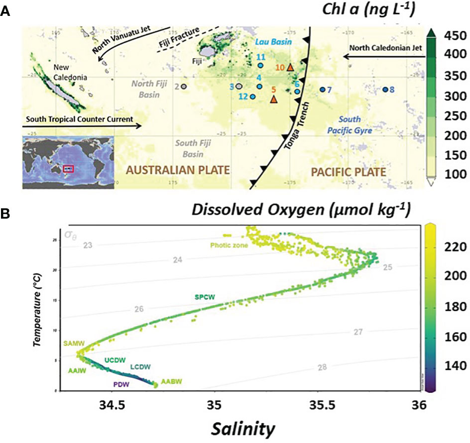
Figure 1 (A) Location of the TONGA GPpr14 expedition superimposed on a time average map of chlorophyll a concentrations from satellite data (ng L^-1; 8-daily 4-km over 2019-11-09 – 2019-12-09) in the Western Tropical South Pacific Ocean (WTSP). Figure generated using Giovanni (giovanni.gsfc.nasa.gov). Numbers represent sampled stations. Grey dot indicates the station sampled in the Melanesian waters (SD 2 and 3), light blue dots the stations sampled in the Lau Basin (stations SD 4, 11 and, 12) and dark blue dots for the stations of the South Pacific Gyre (SD6, 7 and 8). Orange triangles show the location of the two volcanic sites identified (LD 5 and 10). Main surface currents are indicated by black arrows which also mark the Tonga Trench. (B) Temperature-Salinity diagram of the study area with the color corresponding to associated dissolved oxygen concentrations (O₂ expressed in µmol kg^-1). Grey lines indicate the potential densities (referenced to a pressure of 0 dbar). Water masses defined on T-S diagrams are indicated (see text for abbreviations). Figure generated using ODV software (Schlitzer, 2022).

Sampling was operated using a trace metal clean polyurethane powder-coated aluminum frame rosette (TMR) equipped with twenty-four 12 L Teflon-lined GO-FLO bottles (General Oceanics) and attached to a Kevlar® wire. Potential temperature (θ), salinity (S) and dissolved oxygen (O₂) were retrieved from the conductivity–temperature–depth (CTD) sensors (SBE9+) deployed on the TMR. The cleaning protocols of all the sampling equipment followed the guidelines of the GEOTRACES Cookbook (http://www.geotraces.org). After recovery, the TMR was directly transferred into a clean container equipped with a class 100 laminar flow hood. Samples were then taken from the filtrate of particulate samples (collected on acid-cleaned polyethersulfone filters, 0.45 μm supor). For L_FeHS, L_Fe and DOC, the filtrate was collected into acid-cleaned and sample-rinsed high density polyethylene (HDPE) 125 mL bottles. Immediately after collection, samples were double-bagged and stored at -20°C until analysis in a shore-based laboratory. For DFe, the filtrate was collected into acid-cleaned and sample-rinsed 60 mL HDPE Nalgene bottles, acidified to pH ∼1.7 with Ultrapure HCl (0.2% v/v, Supelco®) within 24 h of collection and stored double-bagged pending analysis at Laboratoire d’Océanographie de Villefranche (full protocol and data in Tilliette et al., 2022).

2.2 Reagents

All aqueous solutions and cleaning procedures used ultrapure water (resistivity > 18.2 MΩ.cm^-1, MilliQ Element, Millipore®). An acidic solution (hydrochloric acid, HCl, 0.01 M, Suprapur®, >99%) of 1.24 µmol L^-1 Fe (III) was prepared daily from a stock solution (1 g L^-1, VWR, Prolabo, France). The borate buffer (H₃BO₃, 1M, Suprapur®, Merck, Germany, 99.8%) was prepared in 0.4 M ammonium solution (NH₄OH, Ultrapure normatom, VWR Chemical, USA, 20-22%). The potassium bromate solution (KBrO₃, 0.3 M, VWR Chemical, USA, ≥ 99.8%) was prepared in ultrapure water. Suwannee River Fulvic Acids (SRFA, 1S101F) were purchased at the International Humic Substances Society (IHSS). The SRFA standard stock solution (22.86 mg SFRA L^-1) was prepared in ultrapure water and saturated with iron according to its iron binding capacity in seawater determined by Sukekava et al. (2018). Saturated SRFA solution was equilibrated overnight before its use. Exact concentration of the SRFA stock solution was determined by size exclusion chromatography analysis (Dulaquais et al., 2018b). A 10^-3 M Gallic Acid (GA) stock solution (Sigma-Aldrich) was prepared in HPLC grade methanol, as described in González et al. (2019). The second GA stock solution (10^-6 M) was prepared in ultrapure water. The second stock solution of GA was divided into two portions, with one portion saturated with Fe (final concentration of 5 10^-6 M Fe). Following an overnight equilibration, the Fe-saturated solution was filtered through a 0.02 µm filter to remove any excess iron that precipitated as FeOx.

FeOx dissolution experiments. Artificial seawater (Salinity = 35; pH = 8.2 ± 0.05) was prepared by dissolving sodium chloride (NaCl, 6.563 g, ChemaLab NV, Belgium, 99.8%), potassium chloride (KCl, 0.185 g, Merck, Germany, 99.999%), calcium chloride (CaCl₂, 0.245 g, Prolabo, France, > 99.5%), magnesium chloride (MgCl₂, 1.520 g, Merck, Germany, 99-101%), magnesium sulfate (MgSO₄, 1.006 g, Sigma-Aldrich, USA, ≥99%) and sodium bicarbonate (NaHCO₃, 0.057 g, ChemaLab NV, Belgium, >99.7%) in ultrapure water (250 mL). Artificial seawater was then UV irradiated for 2 hours in order to remove all traces of organic compounds.The UV system consisted of a 125-W mercury vapor lamp with 4 30-mL PTFE-capped quartz tubes (http://pcwww.liv.ac.uk/~sn35/Site/UV_digestion_apparatus.html).

2.3 Analysis of iron-binding ligands of humic type and of dissolved iron-humic concentrations

The determination of L_FeHS was performed on 213 samples from the eight SD and on the two LD stations, including all LD substations, with half the depth resolution. L_FeHS is based on the determination of electroactive humic substances (eHS). Analyses were operated by cathodic stripping voltammetry (CSV) using a polarographic Methrom 663VA stand connected to a potentiostat/galvanostat (µautolab 2, Methrom®) and to an interface (IME 663, Methrom®). Data acquisition was done using the NOVA software (version 10.1). The method used in this study was initially developed by Laglera et al. (2007) and adapted by Sukekava et al. (2018). The method is based on the adsorption at pH 8 of a Fe-humic complex at the surface of a mercury drop electrode under a potential fixed at -0.1 V (vs Ag/AgCl) and its reduction during linear stripping of potentials (0.1 to 0.8 V). In the presence of 30 mmol L^-1 bromate, the reduction of the Fe-humic complex provides a quantitative peak at -0.5 V (vs Ag/AgCl) with an intensity proportional to the concentration. In this study, the samples were defrosted at 4°C and 100 mL were poured in a 250 mL Teflon® bottle. pH was then set to 8.00 ± 0.05 by addition of a borate buffer (final concentration = 10 mM) and adjusted by small additions of an ammonia solution. A first aliquot of the sample was poured into Teflon® vials (Savillex®) in order to detect the natural iron-humic complex (Sukekava et al., 2018). The sample (remaining in the 250 mL Teflon® bottle) was then spiked with 10 nmol L^-1 of Fe to saturate all eHS (and others L_Fe) in the initial sample. After equilibration (1h), 3 others aliquots (15 mL) of the sample were placed into 3 Teflon® vials (Savillex®). Among them, two were spiked with a SRFA standard (1S101F; standard additions of 50 and 100 µg L^-1, respectively) and left for overnight equilibration. After equilibration, the 4 aliquots of samples (1 without Fe, 1 with Fe and 2 with Fe and SRFA additions)were successively placed into a Teflon® voltammetric cell and analyzed by linear sweep voltammetry as described above after 180 s of nitrogen (N₂) purge (Alphagaz®, Air liquide) and a 90 s deposition step at – 0.1V. The absence of quantitative signals in MilliQ water ensured no contamination along the entire analytical process. Peak heights were extracted to determine the electroactive humic concentrations (determined in µg eq-SRFA L^-1). Errors of these measurements were determined using a least-squares fit function. We converted eHS concentrations into L_FeHS, as described by Sukekava et al. (2018), using the binding capacity of the model humic-type ligand SRFA used (1S101F) for DFe in seawater (14.6 ± 0.7 nmol Fe mgSRFA^-1; Sukekava et al., 2018). Similar conversions have been previously used in the recent literature (Dulaquais et al., 2018a; Laglera et al., 2019; Whitby et al., 2020b; Fourrier et al., 2022). The limit of detection (LOD) for 90 s of deposition time was calculated as three times the mean standard deviation of all samples analyzed (n = 213). LOD was estimated at 0.11 nmol eq-Fe L^-1. After data treatment, 12 samples were below the calculated LOD. These samples were mostly within the 200-1000 m depth range where L_FeHS displays their minimal concentrations (Figure 2). They were discarded from the dataset resulting in 201 datapoints for L_FeHS.

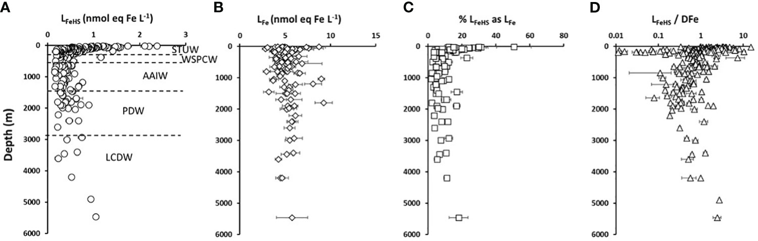
Figure 2 Vertical distribution with depth of (A) humic type ligands (circles, L_FeHS, n = 203), (B) Iron binding ligands (diamonds, LFe, n = 103) and (C) % L_Fe of humic nature (squares,n = 103) measured along the water column during the TONGA expedition. (D) L_FeHS over DFe ratio (triangles, L_FeHS/DFen = 203). Water masses identified by multiparametric optimal analysis and their associated depths are indicated in (A) see text for water masses acronyms.

Voltammetric peaks of the first (i0, pH adjusted sample) and second (i1, pH adjusted and Fe saturated) aliquots permits the determination of the initial amount of DFe bound to humic-type ligands in the sample. This was determined according to equation (1), first introduced by Sukekava et al., 2018.

As no DFe-HS blank signal can be determined (several samples with no i0 signal), the LOD was defined as three times the standard deviation of the lowest DFe-HS concentration ([DFe-HS]) measured (0.01 ± 0.01 nmol eqFe L^-1) and was estimated to be 0.03 nmol eq-Fe L^-1. After data treatment, 14 samples had a [DFe-HS] below the calculated LOD; they were removed from the dataset resulting in 187 datapoints for DFe-HS.

Further discussion about the the relevance of the methodology to determine L_FeHS can be found in the Supplementary Information.

2.4 Dissolution of iron oxyhydroxide by L_FeHS

Experimental dissolutions of FeOx by humic-type ligands were carried out as a function of time and age of FeOx. 250 mL of UV irradiated artificial seawater was spiked with 100 nmol L^-1 Fe. In the absence of organic ligands, the limit of solubility of DFe is subnanomolar (Liu and Millero, 2002), thereby DFe would rapidly form Fe oxyhydroxides (Rose and Waite, 2003b). Fe-spiked artificial seawater was then placed on an agitation table (320 rpm, IKA^®KS basic) all along the duration of the experiment. After intense shaking by hand (10 s), a single aliquot (1.5 mL) of Fe-spiked artificial seawater was sampled at 1 min, 1 h, 6 h and every day over the course of one week and then at two weeks after FeOx initial formation. Aliquots of the FeOx solution were directly transferred to 13.5 mL of a SRFA solution (buffered pH = 8.00 ± 0.05, final concentration 0.5 mg-SRFA L^-1 in UV irradiated artificial seawater) in a Teflon voltammetric cell. After an initial N₂ purge of 180 s, the dissolution kinetic of FeOx by SRFA was followed by CSV during 30 cycles using the same voltametric conditions as described in section 2.3 with N₂ purge and deposition times set at 15 s and 90 s, respectively. The experiment was run in duplicate and was reproducible ensuring reproducibility of the experiment. Measurement of pH at the end of the experiment indicated no significant variation, confirming the stability of the pH within the voltammetric cell throughout the duration of the experiment (1 hour).

2.5 Competition between natural humic-type ligands with gallic acid for iron complexation

The Fe-binding strength of natural humic-type ligands was determined by ligand competition experiments between natural samples and gallic acid (GA). Experiments were conducted on (1) surface seawater collected at 25 m at station 6 (outside the Lau Basin). The experiment (see design of experiment in supplementary information) is based on the measurement of the FeHS voltammetric signal in the same sample that has undergone different additions of DFe and/or GA. The binding properties of GA for Fe (III) used are those described in González et al. (2019) (L_FeGA = 2.75 nmol Fe nmol GA^-1; LogK_FeGa = 9.1).

The competition for Fe’ is based on the equilibrium between DFe and L_FeHS (equation 2) and between DFe and GA (equation 3).

With K_FeHS and K_FeGA, the conditional stability constants of natural humic-type ligands and of gallic acid for DFe, respectively, [DFeHS]; the concentration of Fe bound to natural humic type ligands calculated using the binding capacity of SFRA, [L_FeHS]′; the unsaturated humic-type ligand concentration; [Fe]′, the inorganic Fe species; [DFeGA], the concentration of Fe bound to gallic acid and [GA]′, the concentration of unsaturated Gallic acid ligands.

When the two ligands are in competition, the conditional stability constant of the natural humic-type ligands can be calculated according to equation 4.

The FeHS voltametric signal increasing linearly with Fe, the Fe concentration complexed by humic-type ligands can be determined as the ratio between the FeHS signal for a given experimental condition and the FeHS signal of the samples when saturated with dFe (L_FeHS) multiplied by the binding capacity of the sample (see equation 1). Assuming that eHS only complex with Fe, the free humic-type ligands can be then determined using equation 6.

Assuming that Fe" is negligible over DFe, the concentration of FeGA complex can be estimated using equation 7.

Assuming that GA only complex Fe, when GA is added with a known concentration in a sample, [GA′] can be calculated from the total concentration of added GA (L_{FeGA sample}) according to equation 8.

2.6 Dissolved iron analysis

DFe concentrations were measured by flow injection and chemiluminescence detection (FIA-CL) in a clean room at the Laboratoire d’Océanographie de Villefranche. The method, data and analytical performance are fully presented in Tilliette et al. (2022). The DFe-rich samples were diluted in DFe-depleted seawater collected at SD 8. The final concentration of those diluted samples did not exceed 5 nmol L^-1 and a 0-5 nmol L^-1 calibration curve was used in that case. Each sample was analyzed in triplicate. The mean analytical blank was 21 ± 22 pM and the detection limit was 16 ± 7 pM. Method accuracy was evaluated daily by analyzing the GEOTRACES Surface (GS) seawater (DFe = 0.510 ± 0.046 nmol L^-1; n = 24) which compares well with community consensus concentrations of 0.546 ± 0.046 nmol L^-1.

2.7 Analysis of dissolved organic carbon concentrations

Dissolved organic carbon concentrations were determined by size exclusion chromatography with multi-detectors according to the methodology described in Fourrier et al. (2022). Accuracy of measurements were checked by analyzing deep sea reference samples (DSR, Hansell lab, Florida) each set of ten samples.

2.8 Analysis of iron-binding ligands

Iron-binding ligands (L_Fe) were determined for 103 samples by Mahieu et al. (this issue) using competitive ligand exchange with adsorptive cathodic stripping voltametry (CLE-ACSV). The theory of the CLE-ACSV is presented with great detail in the literature (e.g. Gledhill and van den Berg, 1994; Rue and Bruland, 1995; Abualhaija and van den Berg, 2014; Gerringa et al., 2014; Pižeta et al., 2015). For acquisition of L_Fe data, samples were buffered at pH of 8.2 (1 M boric acid, in 0.35 M ammonia) and separated in 16 aliquots. Then natural ligands were left to equilibrate with DFe levels of 0, 0, 0.75, 1.5, 2.25, 3, 3.5, 4, 4.5, 5, 6, 7, 8, 10, 12 and 15 nmol.L^-1 in the 16 aliquots. The artificial ligand added was salycilaldoxime (SA; 98%; Acros Organics™) at final concentration of 25 µmol.L^-1 resulting to a detection window (D) of 79 (Buck et al., 2007). Analyses were operated on a 663 VA stand (Metrohm™) under a laminar flow hood (class-100), supplied with nitrogen and equipped with a mercury drop electrode (MDE, Metrohm™), a glassy carbon counter electrode and a silver/silver chloride reference electrode (3M KCl) in a Teflon voltametric cell. During the voltammetric measurement, the sample was kept oxygenated by a constant air-flow at the surface and the nitrogen gas flow from the 663 VA stand above the sample was stopped. Detailed procedure can be found in Mahieu et al. (this issue).

2.9 Statistics

A Shapiro-Wilk test was used to verify that the data follows a normal distribution, and the homogeneity of variances was assessed by conducting a Levene’s test. Significance in linear regression analysis was determined using the Pearson test. In cases of normally distributed datasets, the significance of differences between data was examined using t-tests. For non-normally distributed datasets, a non-parametric Wilcoxon-Mann Whitney test was utilized to evaluate the significance of differences. A probability value (p) less than 0.05 was considered statistically significant for all analyses.

3 Results

3.1 Hydrography and hydrothermal context

Three distinct basins were crossed and sampled during the TONGA expedition (Figure 1A). The Melanesian waters (grey dots, SD2 and 3), the Lau Basin (average depth shallower than 2000 m) (Figure 1A, clear blue dots and orange triangles, SD4, 11 and 12, LD5 and 10) and the South Pacific Gyre, east of the Tonga Kermadec Arc (dark blue dots, SD 6, 7 and 8). In the Lau Basin, two shallow volcanic systems hosting hydrothermal sites were studied (Figure 1, orange triangles), referred to LD 5 and LD 10. The hydrothermal system at LD 5 was active and marked by high DFe concentrations, up to 50 nmol L^-1, close to the vent (Tilliette et al., 2022). In contrast, the activity at LD 10 had likely been considerably slowed down at time of sampling, possibly due to the eruption of the nearby Late’iki volcano (Plank et al., 2020). Nevertheless, LD 10 water composition was probably impacted, at least for DFe, by the volcanic activity of the shallow hydrothermal site in the upper 300 m and of Metis at depths deeper than 1000 m (Tilliette et al., 2022; Tilliette et al., sub.).

Low surface chlorophyll a concentrations (< 0.2 mg m^-3 derived from satellite data, MODIS-Aqua MODISA simulations, Figure 1A) and extremely low nutrient concentrations (NO₃^- and PO₄^3-< 50nmol L^-1, https://www.seanoe.org/data/00770/88169/) reflect the ultra-oligotrophy of the North Fiji basin and South Pacific Gyre at the time of sampling. The Lau Basin was marked by higher surface chlorophyll a concentrations than the subtropical gyre (Figure 1) indicating that primary production was enhanced in this area. Bonnet et al. (accepted) have shown the causal link between this increased productivity due to diazotrophic organisms whose iron needs are very important and the shallow hydrothermal sources that bring the necessary iron to the surface.

The water masses along the transect area were extensively studied in Tilliette et al. (2022) using hydrographic properties collected during the TONGA expedition as well as a multiparametric optimal analysis (OMP). The main thermocline (200-700 m) includes the Surface Tropical Underwater (STUW) and the Western South Pacific Central Water (WSPCW). The STUW originates from the subduction of high salinity waters from the equatorial part of the subtropical gyre and is associated with a shallow salinity maximum. Created by subduction and diapycnal mixing, the WSPCW exhibits a linear relationship between temperature and salinity over a wide range up to the intermediate layer. The intermediate layer (700-1300 m) was composed solely of AAIW, a low salinity water mass originating from the sea surface at sub-Antarctic latitudes and characterized by a minimum salinity reached at 700 m. AAIW circulates around the subtropical gyre from the south-east Pacific, spreading north-westwards as tongues of low-salinity, high-oxygen water, and enters the tropics in the western Pacific. The deep layer (> 1300 m) contains the Pacific Deep Water (PDW) and the Lower Circumpolar Deep Water (LCDW). The PDW originates from the equatorial Pacific and flows southwards. It is formed in the interior of the Pacific from upwelling of Antarctic Bottom Water (AABW). PDW is characterized by low oxygen content and well-mixed temperature and salinity. LCDW originates from the Southern Ocean and overlaps the depth and density ranges of PDW. However, it differs from the PDW by a maximum of salinity and oxygen. The OMP results revealed a uniform distribution of water masses along the transect, except the two deep water masses, PDW and LCDW, for which differences could be observed in their distribution west and east of the Tonga Arc. STUW is mainly present at depths between 150 and 300 m, followed by WSPCW which is predominantly present between 300 and 500 m. AAIW dominated the entire transect over a wide depth range from 500 to 1300 m. A major contribution from PDW was found west of the Tonga Arc from 1300 m to the seafloor, while PDW only occupied depths between 1300 and 3000 m east of the arc. Below 3000 m LCDW dominated (Tilliette et al., 2022). It is worth noting that Upper Circumpolar Deep Water (UCDW) and AABW were detected according to their salinity and Temperature (Figure 1) however the OMP operated by Tilliette et al. (2022) revealed a zero contribution from these water masses along the transect.

3.2 Vertical distribution of iron-binding ligands of humic-type

Along the TONGA section, concentrations of L_FeHS ranged from 0.15 ± 0.05 to 2.38 ± 0.05 nmol eq-Fe L^-1 (n = 201; Figures 2A-4A). The lowest concentration was measured at station 6 at 920 m and the highest concentration was detected at station 8 at 25 m in the South Pacific Gyre. At each station, the vertical distribution was similar (Figure 2A) with high concentration (> 1 nmol eq-Fe L^-1) in the upper 55 m (Figure 2A) decreasing with depth in the mesopelagic waters to a relative minimum (L_FeHS< 0.2 nmol eq-Fe L^-1) generally observed between 500 and 1500 m. In the abyssal waters, L_FeHS increased, reaching concentrations close to 0.5 nM eq-Fe (Figure 2A). The interval of concentration and the vertical distribution we report in this work are in good agreement with previous studies reporting humic-type ligand concentrations, including those from the southwestern Pacific (Cabanes et al., 2020). L_FeHS concentrations in the different water masses identified by the OMP are presented Table 1. AAIW was the most depleted (mean_AAIW = 0.33 ± 0.16 nmol eq-Fe L^-1 n = 41) and LCDW the most enriched (mean_LCDW = 0.55 ± 0.31 nmol eq-Fe L^-1 n = 9) in L_FeHS. Titration of iron-binding ligands (L_Fe) over 103 samples provide the complexing capacity of dissolved organic matter for Fe (Figure 2B). L_Fe ranged from 2.8 ± 0.4 to 9.3 ± 1.0 nmol eq-Fe.L^-1 with a mean concentration of 5.2 ± 1.2 nmol eq-Fe.L^-1. The distribution of L_Fe was relatively homogenous along the water column (Figure 2B). The contribution of L_FeHS to L_Fe was calculated as the ratio between both parameters. Among the 103 samples investigated, L_FeHS contributed to between 2% and 51% of L_Fe (Figure 2C) with a mean of 11 ± 8%. The ratio of LFeHS over DFe (Figure 2D) exhibited a wide range of values, spanning from<0.1 to 15.4, with an average of 1.3 ± 1.8. Half of the samples had a ratio below 1, indicating that the organic complexation of DFe by L_FeHS cannot explain alone the observed ambient DFe concentrations along the section. Lower values were observed in the LD5 samples and in the samples collected in the PDW, while higher values were observed in the surface samples and in the LCDW.

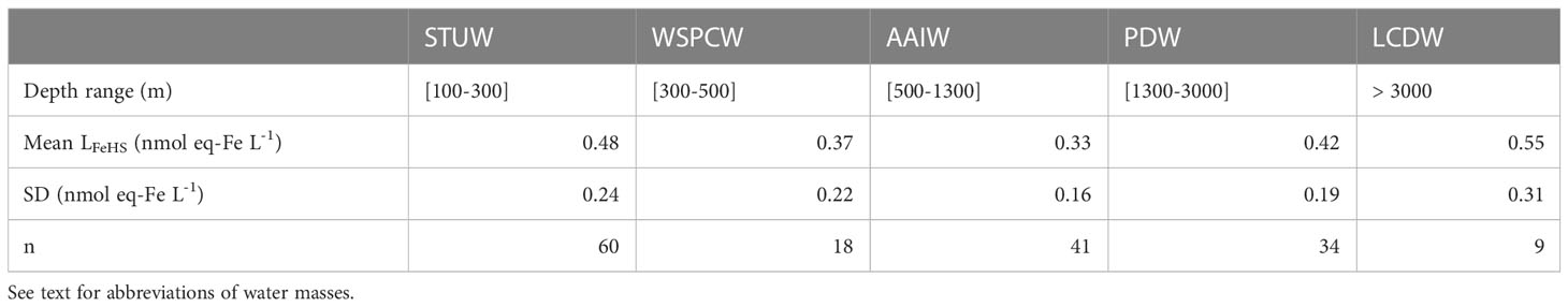
Table 1 Mean concentration of iron binding ligands of humic nature (L_FeHS) and associated variability (SD) measured in the water masses encountered during the TONGA expedition.

3.3 Iron associated with L_FeHS and L_FeHS saturation state

The concentration of Fe complexed by L_FeHS was estimated by considering the saturation state of L_FeHS and the binding capacity (BC) of the external standard used (SRFA 1S101F; BC_SRFA = 14.6 nmol Fe. mg SRFA^-1, Sukekava et al., 2018). Despite the uncertainty of this methodology (see section 2.3), it provides information regarding the amount of DFe associated to L_FeHS. The average calculated DFe-HS was 0.15 ± 0.10 nmol Fe L^-1 (n = 192) and ranged between 0.03 ± 0.02 nmol Fe L^-1 to 0.56 ± 0.04 nmol Fe L^-1. The mean contribution of DFe-HS to DFe was 30 ± 23%. The lowest concentrations were found between depths at depths between 60 and 120 m for four stations (Figures 3C, 4). The highest concentration was recorded at 175 m of substation T4 of LD5 in the vicinity of the hydrothermal plume of LD 5 (Figure 4A). In this latter sample, a DFe peak (~10 nM) associated with hydrothermal activity was recorded by Tilliette et al. (2022) and DFe-HS contributing for 5.5% of total DFe. DFe-HS concentrations were generally lower than 0.2 nmol L^-1 in the upper 200 m, with the exception of LD 5 and LD 10 (Figure 4), and higher than 0.2 nmol L^-1 in the intermediate and deep waters (deeper than 1000 m, Figure 3). The local minima of DFe-HS were generally observed at the depth of the local Chlorophyll maxima (see section 4.4). At these depths DFe-HS accounted for 21 ± 15% of total DFe. The saturation of L_FeHS by Fe is presented in Figure 3D. With the exception of one datapoint at 3500 m at station 7, ambient L_FeHS were not saturated by Fe. The mean saturation state was 37 ± 26% (n = 192), ranging from 3 ± 5% at 25 m at station 8 to up to 102 ± 4% at 3600 m at station 7. Lowest saturation states (< 10%) were found in the upper water, associated with low DFe concentrations (SD 3, 7, 8). This was expected considering the low DFe concentrations (Tilliette et al., 2022) and the high L_FeHS concentrations (Figure 3A). In the Lau Basin, relatively low saturation states of L_FeHS (< 30%, Figure 3D) were observed between 1000 and 1400 m depth. Deeper than 1000 m depth, the saturation of L_FeHS was generally higher than 40% in the Melanesian waters and the south Pacific subtropical gyre. Our results indicate that a large fraction of L_FeHS were not saturated by Fe. These free L_FeHS should be able to support Fe complexation and its stabilization in the dissolved phase if Fe is added to the system by volcanic or hydrothermal activity.

Figure 3 Vertical distribution of (A) Iron binding ligands of humic nature (L_FeHS); (B) dissolved iron (DFe) effectively complexed by L_FeHS (DFe-HS); (C) L_FeHS saturation state (%); (D) Percentage of DFe under DFe-HS (%) with longitude during the TONGA expeditione (GEOTRACES GPpr14). Map of the expedition and the three distinct biogeochemical domains crossed are indicated.

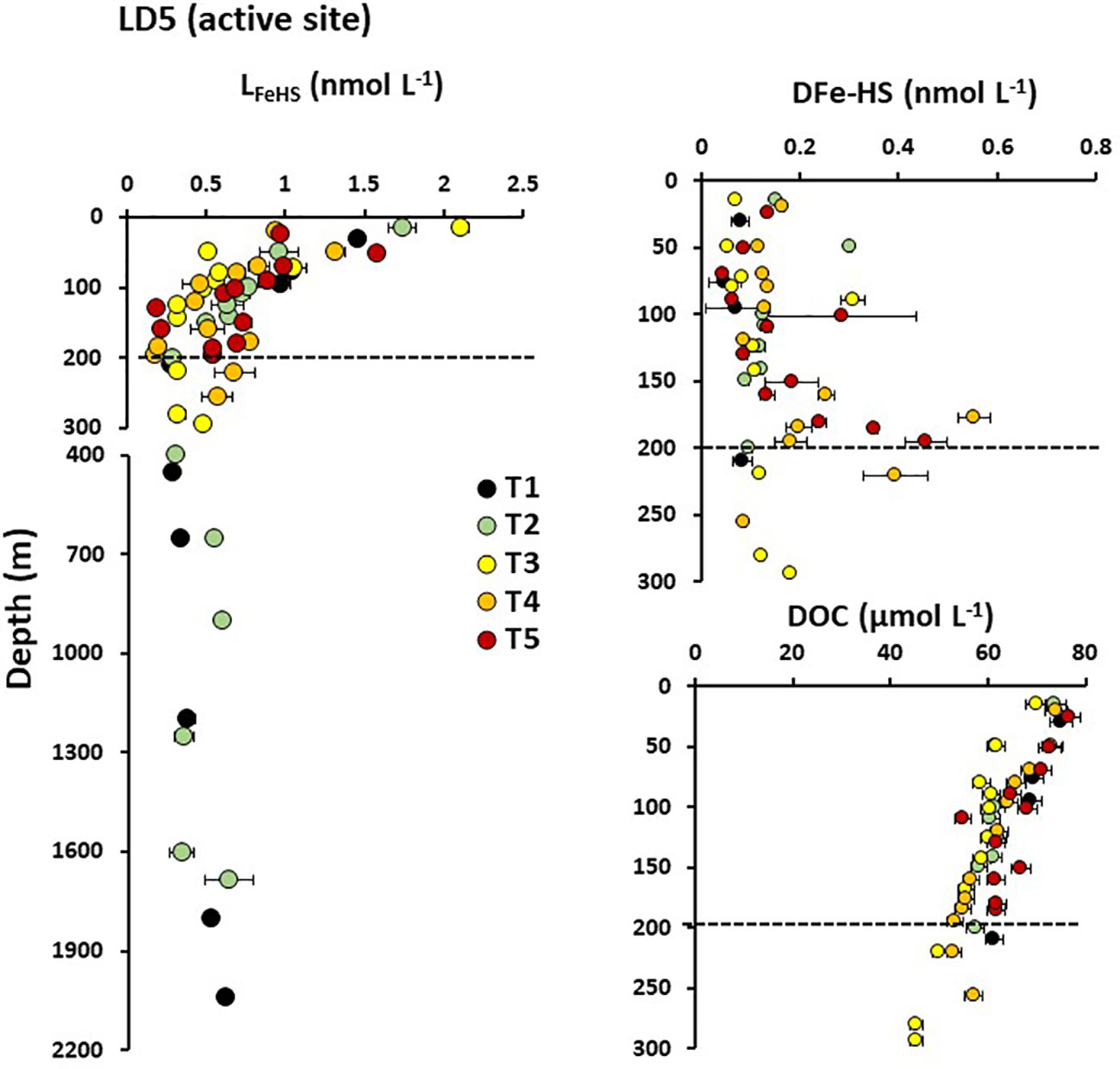
Figure 4 Vertical distribution of humic-type ligand concentrations (L_FeHS) above and in the vicinity of LD 5 hydrothermal site. Dashed lines indicate the approximate depth of the hydrothermal plume at LD 5-T5 (~190 m). Associated concentrations of dissolved iron complexed by L_FeHS (DFe-HS) and of dissolved organic concentrations (DOC) are presented for the upper 300 m.

3.4 L_FeHS and DFe-HS in a hydrothermal system of the Tonga arc

The impact of the hydrothermal activity along the Tonga arc on L_FeHS concentrations and DFe associated with these ligands (DFe-HS) was studied at LD 5 and LD 10. Five and four subcasts were operated at LD 5 and LD 10, respectively, to capture the dispersion of the hydrothermal plume. We focus here on the active site LD5 (Figure 4) where high DFe concentrations (up to 50 nmol L^-1) were measured close to the vent (Tilliette et al., 2022). At the subcasts close to the vent (T5 and T4), L_FeHS and DOC concentrations did not show any significant enrichment at depths where the hydrothermal plume was located (~195 m; Figure 4). Similarly, there was no L_FeHS or DOC enrichment at LD 10 (see Supplementary Information). These results indicate that these hydrothermal systems were not a source of L_FeHS or DOC. In contrast, DFe-HS did show an enrichment at depths where the hydrothermal plume was located (Figure 4B). At T5, the concentration of DFe-HS increased while the saturation of L_FeHS decreased with increasing proximity to the vent, from 0.06 nmol L^-1 (8% saturated with Fe) at 70 m to 0.46 nmol L^-1 (83% saturation) at 195 m depth, nearest the vent. Due to the much higher DFe concentration in the deeper sample (DFe ~50 nmol L^-1 at 195m), only ~1% of DFe was complexed by L_FeHS at this depth. The highest DFe-HS concentration was measured at 175 m depth of T4 (0.56 nmol L^-1) where DFe was ~10 nmol L^-1 with ~5.5% of DFe was present under DFe-HS. Unsaturation of L_FeHS at 195 m of T5 despite the high DFe concentration (~ 50 nmol L^-1) suggests that this hydrothermal DFe was present under a chemical form not fully accessible for complexation by L_FeHS. The increase in DFe-HS concentration during plume dispersion between T5 and T4 (Figure 4B) indicates that complexation of DFe by L_FeHS begins at the onset of hydrothermal mixing and proceeds further during plume dispersion. Our data thus indicate that the complexation of hydrothermal DFe by L_FeHS is a kinetically controlled process.

3.5 Iron oxyhydroxide dissolution by humic-type ligands: from lability to inertness

Hydrothermal systems release large amounts of FeOx to the ocean, thereby we studied the ability of L_FeHS to solubilize FeOx in seawater. For this purpose, a dissolution experiment of FeOx in the presence of a model L_FeHS (SRFA) was carried out (Figure 5A). The experiment consisted of monitoring the formation of the DFe-HS as a function of time and as a function of age of FeOx. Results show that immediately after FeOx formation, amorphous Fe(III) is accessible to L_FeHS generating a quantifiable signal. Within an hour, 40% of initially-formed FeOx were dissolved, demonstrating that L_FeHS can solubilize FeOx with a kinetic rate constant (k) of at least 1.2 10⁶ mol^-1 L min^-1.

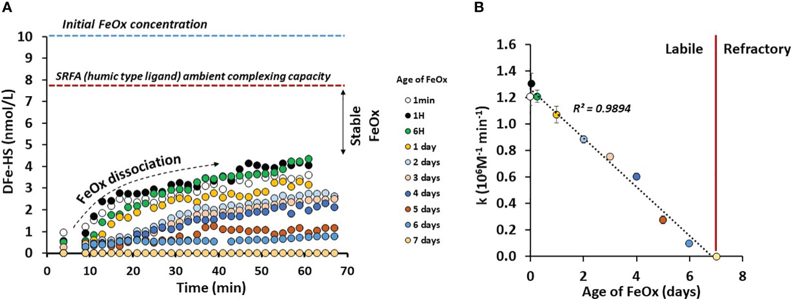
Figure 5 (A) [Fe] (nmol kg^-1) bound by a humic-type ligand (SRFA 1S101F) as a function of time (min) and age of iron oxyhydroxide (FeOx) in artificial seawater. (B) Dissolution rate constant of FeOx (k in µM^-1 min^-1) as a function of FeOx ageing. See text for explanations.

Age of FeOx was however a strong controlling parameter on the dissolution rate. A dramatic linear decrease of k with time (k = 1.25 10⁶ M^-1 - 0.18 * t(d), R² = 0.99, n = 10) was observed (Figure 5B). After 2 days only 2.5 nmol L^-1 over 10 nmol L^-1 of FeOx can be dissolved by SRFA after 1 hour of experiment. After a week of ageing, there was no quantifiable signal after 1 hour experiment (Figure 5A). Additional experiments were carried out two weeks after FeOx formation and no measurable signal was observed (data not shown).

4 Discussion

4.1 L_FeHS cycling in the WTSP

The high concentrations and surface maxima of L_FeHS observed in this area not impacted by continental inputs indicate a marine origin of L_FeHS in these subtropical waters. Direct excretion by phytoplankton is a possible source of L_FeHS (Stedmon and Cory, 2014), however chlorophyll a (derived from CTD fluorescence sensor) and L_FeHS discrete maxima were not observed at the same depth (see section 4.4). The absence of a significant correlation between chlorophyll a and L_FeHS in the upper 200 m (R²< 0.1; p > 0.75, n = 91) suggest an indirect pathway for the production of these ligands. The release of DOM during the degradation of phytoplankton material (cell lysis, grazing) in the first hundred meters combined with its microbial and chemical processing (Obernosterer et al., 1999) are the most probable pathway of production for these ligands. This proposed production pathway is in agreement with in situ experiments from Whitby et al. (2020a) who showed a release of humic-type ligands during microbial respiration of biogenic particulate organic carbon originating from the oligotrophic Mediterranean waters and from the high nutrient low chlorophyll Southern Ocean waters.

The vertical decrease of L_FeHS in the mesopelagic zone (Figures 2A, 3A) reveals the partial degradation of L_FeHS during microbial mineralization of DOM. Direct consumption of humics by heterotrophic bacteria reported in several studies (Cottrell and Kirchman, 2000; Coates et al., 2002; Rosenstock et al., 2005) support our observations. The persistence of L_FeHS in the deep PDW (mean_PDW = 0.43 ± 0.19 nmol eq-Fe L^-1 n = 34) indicate that part of L_FeHS, however, escapes microbial degradation and is refractory. To monitor the effect of microbial mineralization process on L_FeHS, we calculated the apparent oxygen utilization (AOU) based on dissolved oxygen concentrations, S, T (all derived from CTD sensors) using Benson and Krause (1984) formula. AOU is the integrated oxygen consumption by heterotrophic bacteria in the breakdown of organic matter. In the study area, mineralization of labile, semi-labile and semi-refractory DOM can be tracked by the linear decrease of DOC concentration (i.e. proxy of DOM) with increasing AOU down to ~100 µM (R² > 0.57; p< 0.05; n = 133; Figure 6B). At AOU > 100 µmol O₂ kg^-1, DOC concentrations were relatively homogenous (~ 37 µM) indicating that DOC was mostly refractory to microbial respiration. A plot of L_FeHS against AOU also reveals a decrease of humic-type ligand concentration during the mineralization process (Figure 6B). Down to an AOU of 100 µmol O₂ kg^-1 the decrease of L_FeHS was likely driven by a power law (R² > 0.42; p< 0.05; n =133) rather than by direct linear regression. At AOU > 100 µmol O₂ kg^-1, L_FeHS seems to increase with increasing AOU (Figure 6A) but the correlation was not significant (R²< 0.05; p > 0.05; n = 75). A weak but significant correlation between L_FeHS and DOC for AOU > 100 µmol O₂ kg^-1 (Figure 6C; R² > 0.25; p< 0.05; n = 133) was observed indicating that L_FeHS cannot be modeled accurately through an empirical equation based on DOC. The weak correlation between L_FeHS and DOC was expected due to the intrinsec difference between both parameters. On the one hand,DOC consists of a broad pool of molecules that undergo both respiration-driven losses and gradual conversion into refractory compounds (Figure 6B). On the other hand, L_FeHS represents a more specific property (binding sites) of DOM that is primarily lost through microbial turnover (Fourrier et al., 2022).

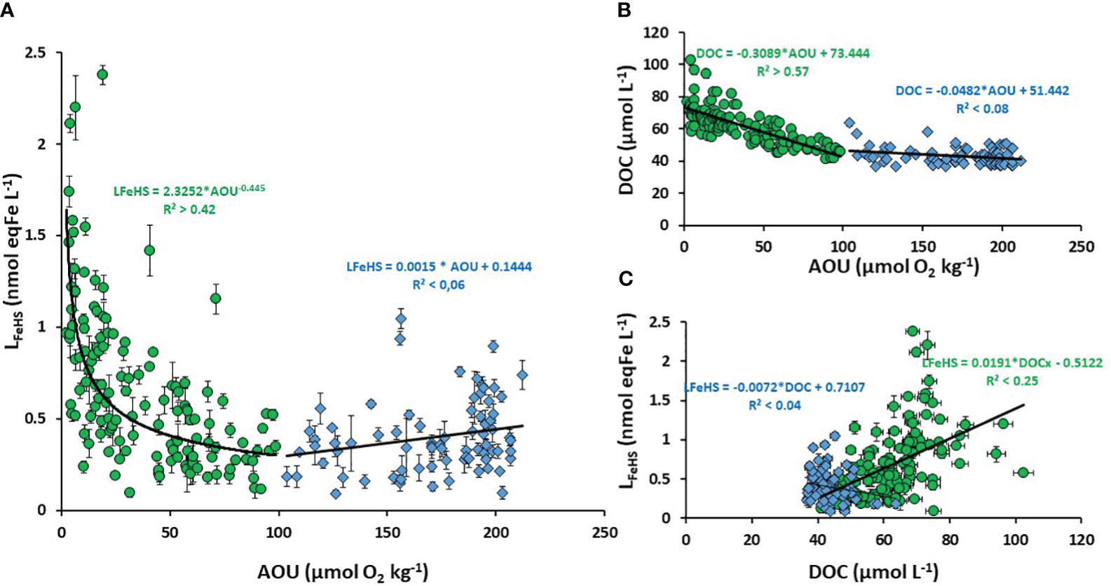
Figure 6 Scatter plot of (A) Humic type ligand (L_FeHS) versus apparent oxygen utilization (AOU); (B) Dissolved organic carbon (DOC) versus AOU; (C) L_FeHS versus DOC. The dataset was separated between low AOU (< 100 µmol O2 kg^-1, green dots) and high AOU (> 100 µmol O2 kg^-1, blue triangles). Associated correlations are indicated.

The contribution of L_FeHS to L_Fe in our study (2% to 51%, Figure 2) is lower compared to the findings of Whitby et al. (2020b) (23-58%) in the North Atlantic Ocean. This disparity can be attributed to both geographical and methodological differences. Whitby et al. (2020b) studied samples from the North Atlantic Ocean, where the presence of terrestrial influence (and the associated humic substances) could potentially lead to high concentrations of L_FeHS. In contrast, the study area of the WTSP lacks terrestrial influence, resulting in the absence of a terrigenous component and lower concentrations of L_FeHS than in the Atlantic. Furthermore, our study used SA as the competing ligand for L_Fe titration, while Whitby et al. (2020b) used 2-(2-Thiazolylazo)-p-cresol (TAC). It is important to note that TAC may not fully capture the contribution of humic-type ligands (as highlighted by Laglera et al., 2011 and Slagter et al., 2019). Therefore, the values reported by Whitby et al. (2020b) might represent the minimum concentration of the ligand pool, underestimating the actual presence of humic substances. These factors account for the higher L_FeHS contribution reported by Whitby et al. (2020b) in the North Atlantic compared to our study.

4.2 Classification of L_FeHS and iron speciation within L_FeHS in the western Pacific Ocean

The L_FeHS concentrations measured during this study were lower than the total iron binding ligand (L_Fe) concentration measured by CLE-CSV (Figure 2). Over the 103 common samples analyzed by CLE-CSV and L_FeHS, the mean log ${\text{K}}_{\text{FeL},\text{Fe}\text{'}}^{\text{cond}}$ was 11.6 ± 0.4 ranging from 10.5 ± 0.2 to 12.7 ± 0.3. According to the classification defined by Gledhill and Buck (2012), 84% of samples fall in the L₂ class, 13% in the L₁ class, and 4% in the L₃ class (Mahieu et al., this issue). This result clearly indicate that intermediate class ligands (L₂) dominated the pool of L_Fe all along the water column in our study area. This is in agreement with the previous datasets reported by Buck et al. (2018) and Cabanes et al. (2020) in the oligotrophic South Pacific Ocean. Cabanes et al. (2020) also measured L_FeHS, and showed that the weakest class of ligand (log ${\text{K}}_{\text{FeL},\text{Fe}\text{'}}^{\text{cond}}$ < 11) observed was associated with the lowest humic-type ligand concentration. All these observations indicate that the L_FeHS measured here are ligands of intermediate strength (L₂ type). However, classifying based on log ${\text{K}}_{\text{FeL},\text{Fe}\text{'}}^{\text{cond}}$ does not capture the heterogeneity of binding sites for non-discrete ligands like L_FeHS. To mitigate biases introduced by CLE-CSV, it is preferable to use αFeL(Fe’) (reactivity coefficients) for studying the nature of LFe (Gledhill and Gerringa, 2017).

To study the nature in term of strength of L_FeHS, we conducted competitive ligand experiments for Fe complexation between ambient natural ligand including L_FeHS and Gallic Acid (GA) to study the mobility of Fe and its speciation within the Fe-humic complex. According to the only available published data from González et al. (2019), GA in seawater is a weak Fe ligand (log K_FeGA = 9.1) with a binding capacity of 2.75 nmol eq-Fe nmol GA^-1. We choose this ligand for two reasons. Firstly, GA is a polyphenolic compound with a carboxylate moiety. Phenolic and carboxylates are thought to be the moieties involved in the formation of the Fe-humic complex (Garnier et al., 2004; Hassler et al., 2019). GA is thus a good candidate to compare the affinity of Fe for humic substances with these moieties. Secondly, GA reduces Fe(III) into Fe(II) with time (González et al., 2019; Pérez-Almeida et al., 2022). The affinity of marine humic type ligand for Fe(II) can then be studied after i) the saturation of GA with Fe, ii) equilibrium to allow the reduction of Fe(III) into Fe(II) by GA, and competition ligand experiment.

The sample used for this experiment has an initial DFe concentration of 0.45 ± 0.01 nmol L^-1; L_Fe was 4.8 ± 0.5 nmol eq-Fe L^-1 with an associated log ${\text{K}}_{\text{FeL},\text{Fe}\text{'}}^{\text{cond}}$ of 11.8 ± 0.4 (Mahieu et al., this issue). L_FeHS was estimated at 1.52 ± 0.02 nmol eq-Fe L^-1, 32% of L_Fe. The initial DFe-HS was 0.18 nmol L^-1. If we consider all DFe to be labile for organic complexation, the initial conditions of the experiment can be described as follows: (i) L_Fe′ and L_FeHS′ were respectively 4.3 and 1.34 nmol eq-Fe L^-1, (ii) 0.27 nmol L^-1 DFe were complexed by non-humic L_Fe and (iii) the log αFeL(Fe′) (e.g. side reaction coefficient) was 3.4. A first experiment consisted of the addition of 1.6 nmol L^-1 of Fe to the sample. After 20 h of equilibration, DFe-HS reached 1.50 ± 0.05 nmol L^-1 thereby L_FeHS were at saturation. Considering the ambient L_Fe concentration of the sample, determined by CLE-ASV, our results demonstrate that the Fe added went primarily into L_FeHS. CLE-ACSV analysis only provides an average lo ${\text{K}}_{\text{FeL},\text{Fe}\text{'}}^{\text{cond}}$ g of the ligand pool (captured by the detection window of the method) but the L_Fe pool is composed of a wide variety of organic compounds with different log ${\text{K}}_{\text{FeL},\text{Fe}\text{'}}^{\text{cond}}$ (Town and Filella, 2000). The log ${\text{K}}_{\text{FeL},\text{Fe}\text{'}}^{\text{cond}}$ of 11.8 ± 0.4 measured for the sample studied is an average of the ligand pool that is composed of ligands and binding sites with both higher and lower strength than this average value.

Considering the initial conditions, it can be inferred that approximately 0.43 nmol eq-Fe L^-1 of the L_Fe pool, including 0.18 nmol eq-Fe L^-1 of L_FeHS, have log αFeL(Fe’) values higher than 3.4, indicating the potential presence of L₁ type binding sites (estimated mean log ${\text{K}}_{\text{FeL},\text{Fe}\text{'}}^{\text{cond}}$ ≥ 12.8). Since the addition of DFe initially fills the remaining free sites of L_FeHS, our results suggest that the log αFeL_FeHS(Fe’) values for the binding sites in L_FeHS that were not initially filled with DFe are at least equal to 3.4 (estimated mean log ${\text{K}}_{\text{FeL},\text{Fe}\text{'}}^{\text{cond}}$ ≥ 12.3). Based on the initial conditions and the results of our experiment, a distribution of binding site density within the L_FeHS pool can be inferred. L_FeHS comprises a small portion (12%) of sites with high affinity (L₁ type) that can outcompete strong discrete ligands, while the majority (88%) of sites fall into the L₂ type category, likely at the higher end of the strength scale associated with L₂ type sites. The remaining 3 nmol eq-Fe L^-1 of the L_Fe pool may be considered as weaker ligands compared to L_FeHS. Our findings are consistent with the results reported by Gledhill et al., 2022, who demonstrated that the heterogeneity of binding sites in humic-like DOM enables humic substances to outcompete siderophores at low iron concentrations.

In a second experiment, Fe-free GA was added but the response of DFe-HS was unchanged, showing that the Fe cannot be dissociated from the Fe-humic complex by 2 nmol L^-1 of GA (L_FeGA = 5.5 nmol eq-Fe.L^-1) at a pH of 8.0 (Figure 7). This demonstrate that the affinity of L_FeHS for Fe is higher than 10^9.1 and that polyphenolic and carboxylate moieties of GA cannot outcompete those involved in the complexation of Fe in L_FeHS even at higher GA ligand concentration. This experiment confirms that surface L_FeHS in the WTSP are, at least, ligands of intermediate strength.

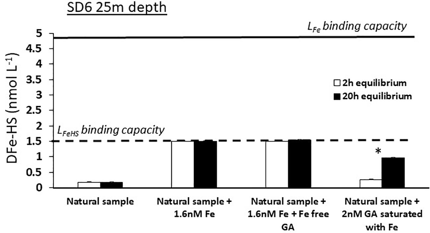
Figure 7 Monitoring of dissolved iron complexed by humic type ligand concentration (DFe-HS) before (white bars) and after(dark bars) overnight equilibration between natural ambient iron-binding ligands (L_Fe), humic-type ligands (L_FeHS) and Gallic Acid (GA) for a surface sample with oligotrophic conditions (SD 6, 25 m depth). Solid and dashed line indicate the iron binding capacity of the ambient L_Fe and L_FeHS. * indicates a significant difference between initial and final DFe-HS concentrations. Absence of iron saturation of L_FeHS in experiments c and c’ and no changes in DFe-HS in experiments d and d’ indicate the instability of Fe(II)-humic ligand complexes and that Fe(III)-humic complexes are of higher stability than Fe-GA complexes. See text for explanation.

In a third experiment, 2 nmol L^-1 of GA saturated with Fe were put in contact with unsaturated L_FeHS (Figure 7). After 20 h of equilibration, L_FeHS were able to dissociate partly Fe from the Fe-GA complex. However L_FeHS but did not reach saturation even with an addition of 5.5 nM of DFe bound to GA (e.g. 5.5 nmol eq Fe L^-1 for 2 nmol L^-1 GA; González et al., 2019). Using equations (2) to (8), this scenario allows to calculate the apparent stability constant of L_FeHS in the condition of the experiment (20°C, pH = 8, 20h of competition). A value of logK_LFeHS = 8.5 ± 0.2 was obtained, much lower than expected from the first two experiments. There are various possibilities to explain these apparent differences:

i) the third experiment was not at equilibrium and the reaction need to be longer than 20h; this hypothesis was disproved by running a similar experiment but with 36h equilibration time; same results were obtained. ii) The Fe-humic complex is metastable and cannot be dissociated even by a stronger ligand; this is unlikely from previous experiments conducted by Laglera et al. (2019) who demonstrated that desferrioxamine B (strong ligand) and EDTA (weak ligand) can both dissociate Fe from a natural Fe-humic complex when their concentrations are sufficiently high. iii) GA partially reduced Fe(III) to Fe(II), because the latter has higher affinity for GA and non-humic L_Fe than Fe(III) has for L_FeHS, resulting in an apparent lower log ${\text{K}}_{\text{FeL},\text{Fe}\text{'}}^{\text{cond}}$. The pH dependence of the Fe-humic reduction peak potential (increasing peak potential E_peak with decreasing pH) observed by Laglera et al. (2007) provide further perspectives for interpretation iii). Their observations indicate that the stability of the Fe-humic complex decreases with decreasing pH. An increasing proportion of Fe(II) at lower pH can explain this shift of E_peak with pH, since Fe(II)-humic complexes have lower stabilities compared to Fe(III)-humic complexes (Rose and Waite, 2003a; Blazevic et al., 2016). Based on our experiments and the studies mentioned above, we suggest here that a Fe-humic complex is only stable in seawater with Fe(III). It can be further hypothesized that to form an Fe-GA complex stable in seawater, Fe should be under Fe(II) in the Fe-GA complex. These conclusions have broader implications for the fate of Fe in environments with low pH and changing redox conditions, such as low oxygenated margins and hydrothermal environments (as observed at LD5 T5, Figure S4), or where photoreduction of Fe is enhanced (e.g. clear subtropical waters).

4.3 The role of L_FeHS in the stabilization of hydrothermal DFe

The kinetic monitoring of FeOx dissolution by L_FeHS demonstrates that the age of FeOx is a main factor controlling their dissolution rate (Figure 5). The experiment we conducted shows that recently formed FeOx are very labile but become gradually refractory to dissolution by L_FeHS with time; the studied model humic-type ligand was not able to solubilize FeOx aged one week or more (Figure 5). A similar effect of ageing on the solubilization of FeOx was observed for desferoxiamine B (Rose and Waite, 2003b) with a nearly 50 times decrease of the dissolution rate constant after a week of FeOx maturation. Our results are also in line with those of Krachler et al. (2015) who observed a rapid dissolution of newly formed FeOx by a set of L_FeHS and experiments by Tani et al. (2003) that correlated the solubilization of newly formed FeOx with humic-like fluorescence in seawater. In contrast, Kuma et al. (1996) did not see such a strong effect of age on FeOx solubility probably due to inherent differences in methodologies. They added FeOx in natural seawater and followed their solubility over time, which is equivalent to studying the stability of organically complexed DFe originating from the dissolution of newly formed FeOx.

In hydrothermal environments, most DFe is released under the form of soluble Fe(II). The fraction of DFe that escapes precipitation of sulfide minerals (e.g. pyrite, chalcopyrite) is then gradually oxidized and forms insoluble Fe (III) oxyhydroxides species (FeOx) both under colloidal and particulate form (Lough et al., 2019; Cotte et al., 2020; Hoffman et al., 2020). Recent studies highlight the high proportion of colloidal DFe in hydrothermal plume at dozens to hundreds of kilometers from the vent (Tagliabue et al., 2022; Lough et al., 2023). However the persistence of DFe plumes at great distances from deep vents is often explained by its initial stabilization under an organic form (Sander and Koschinsky, 2011; Hawkes et al., 2013; Wang et al., 2021; Wang et al., 2022). In the first stage of hydrothermal mixing, DFe occurs essentially as Fe(II) species (Waeles et al., 2017). With Fe(II) having low affinity for L_FeHS, (Figure 7; Rose and Waite, 2003a), the pathway of Fe-HS formation in hydrothermal plumes requires the oxidation of Fe(II) to Fe(III), through the formation of colloidal Fe oxides species that may be partly dissolved by L_FeHS. Our experiments strongly suggest that dissolution of FeOx by humic-type ligands is only possible during the first hours or days after precipitation (Figure 5). Ligand concentration is not the only factor controlling the solubility of FeOx as shown by our lab experiments and field observations (unsaturated L_FeHS in the presence of high DFe concentrations, Figure 4). Therefore, the kinetics of the plume dispersion must be taken into account when studying the organic complexation of hydrothermal Fe. The persistence within the DFe fraction of colloidal FeOx observed in the widespread hydrothermal plume of the Pacific Equatorial Ridge (Fitzsimmons et al., 2017) is in agreement with our observations and support our conclusions. It is worth noting that our dissolution experiments were achieved in UV digested artificial seawater, neglecting key parameters of the hydrothermal environment (e.g. pH, O₂, pressure, temperature, DOC, sulfide, other trace metals) that may impact the nature, concentrations, kinetics of formation, stability and transport of these Fe colloidal species. For instance, the composition of the fluid, dissolved O₂ concentrations, pH, temperature and local currents driving plume dilution are parameters to be considered for Fe oxidation and mineral formation (Byrne et al., 2000; Field and Sherrell, 2000; Shaw et al., 2021; Tilliette et al., 2022). Although not representative of the natural hydrothermal system, our dissolution kinetics experiments provide valuable insights into the processes involved.

At LD5, we observed that L_FeHS stabilized a very small fraction of the DFe released by the hydrothermal vent (Figure 4) keeping unsaturated L_FeHS in the presence of high DFe (~50 nmol L^-1). This inability of L_FeHS to complex DFe released at LD5-T5 might be due to the low pH (< 6.5) and low O₂ (< 160 µM) values at this site, resulting in a seawater relatively acidic and suboxic (Tilliette et al., 2022; Figure S4). Under these conditions, a significant fraction of Fe(II) may persist which has low affinity for L_FeHS. In addition, the fraction of DFe stabilized by L_FeHS increased from 1 to 5.5% between substations T5 and T4 while a majority (78%) of the DFe released precipitated in the first 600 m (Tilliette et al., 2022). During its dispersion in shallow waters, the plume is rapidly diluted with more alkaline, more oxygenated and warmer seawater that will favor the formation of FeOx species (Figure S4). This newly formed FeOx may be dissolved by L_FeHS (Figure 5) at a rate that is at least dependent on the age of these FeOx as well as the concentration of Fe-free L_FeHS (Figure 5) and certainly on many other parameters (concentration of particles, concentration of other dissolved metals, DOC, plume dispersion, etc). It is worth noting that pH and temperature play crucial roles in iron organic complexation and FeOx formation (Byrne et al., 2020; Ye et al., 2020; Zhu et al., 2021). Considering the significant variations in these parameters within hydrothermal environments (Figure S4), it is recommended to design further experiments to gain a better understanding of the impact of pH and temperature on the dissolution of FeOx by L_FeHS.

4.4 Bioavailability of DFe-HS and stabilization of DFe by L_FeHS in intermediate and deep waters of the WTSP

For data interpretation, samples with DFe concentrations exceeding 2 nnmol L^-1 were identified as being influenced by the hydrothermal system and were subsequently excluded from the depth horizons discussed in the following sections. In the first 50 m of the water column, above the deep chlorophyll maximum (Above DCM, Chl a< 0.075µg L^-1), L_FeHS was high (mean_{Above DCM} L_FeHS > 1.2 ± nmol eq-Fe L^-1 n = 18; Figure 8A) and DFe-HS concentrations were relatively low (mean_{Above DCM} DFe-HS = 0.18 ± 0.12 nmol L^-1 n = 18; Figure 8B) resulting in a low saturation of L_FeHS (17 ± 10%, n = 18 Figure 8C). The non-accumulation of DFe in the presence of high L_FeHS is in stark contrast with what was observed in the Mediterranean Sea (Dulaquais et al., 2018a) and in the Arctic waters (Laglera et al., 2019). This observation suggests that, in the surface water of the WTSP, DFe can be dissociated from the humic complex, becoming available for surface reaction (e.g. scavenging) or biological uptake. It is not clear from our data if DFe is directly removed from the humic complex or if photoreduction of Fe within the complex via ligand-to-metal charge transfer leads to the production of Fe(II) with low affinity for L_FeHS (Figure 5; Barbeau, 2006; Blazevic et al., 2016). An additional process explaining the non-accumulation of DFe within L_FeHS in surface could be the presence of DFe under a colloidal fraction that is not available for complexation with L_FeHS. Colloidal DFe can represent a large fraction of DFe in surface waters of the Pacific ocean (Wu et al., 2001). It is considered poorly bioavailable (Rich and Morel, 1990; Chen and Wang, 2001; Wang and Dei, 2003) but prone to scavenging, limiting its accumulation in surface waters (Kunde et al., 2019). Below 50 m depth, a clear and significant (p< 0.05) depletion of DFe-HS in the deep chlorophyll maximum (DCM, Chl a > 0.1 µg L^-1) over the entire section was observed (mean_DCM DFe-HS = 0.11 ± 0.08 nmol L^-1 n = 49; Figure 8). These very low DFe-HS concentrations clearly indicate that when complexed to L_FeHS, DFe is bioavailable for phytoplankton. However, it is unclear if phytoplankton cells can directly uptake Fe from the humic complex, if phytoplankton species produce specific ligands to outcompete L_FeHS (e.g. EPS, siderophores) or if Fe uptake by the cell is due to remineralisation of the humic-complex (Figure 8). Hassler et al. (2019) classify the model L_FeHS SRFA as a source of bioavailable Fe for a set of phytoplankton species but this has not yet been shown, and laboratory culture experiments should be designed to address these questions of DFe-HS bioavailability that could also arise from the dissociation of DFe-HS, as inorganic DFe is continuously assimilated.

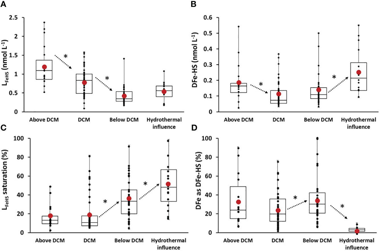
Figure 8 Box and whisker plot of (A) associated iron binding ligands of humic nature (L_FeHS in nmol eq-Fe L^-1); (B) iron effectively associated with L_FeHS (DFe-HS in nmol eq-Fe L^-1); (C) L_FeHS saturation state (%); (D) Percentage of DFe under DFe-HS (%) along the section for 4 specific depths clusters of sample: above the deep chlorophyll maximum (above DCM), the deep Chlorophyll maximum (DCM), below the deep chlorophyll maximum and for samples influenced by hydrothermalism. Black dots represent discrete data. Red dots indicate the mean value of data. * and arrows indicate significance and way of variation between two close depth horizons. Significance were tested using Wilcoxon-Mann Whtiney tests and set for 95% of confidence (p< 0.05) determined by Wilcoxon-Mann Whtiney test.

Below the DCM (Below DCM, Chl a< 0.075 µg L^-1; depth > 100m), DFe-HS concentrations was stable (mean_{Below DCM} DFe-HS = 0.15 ± 0.12 nmol L^-1 n = 38; Figure 8B) and significant (p< 0.05) increase of L_FeHS saturation index (Figure 8C) indicate a stabilization of DFe by L_FeHS after the remineralization of sinking biomass. The contribution of DFe-HS to DFe also increase at these depths (Figure 8D), with the exception of LD5-T5 and T4 due to high DFe, further showing an increased stabilisation of DFe by L_FeHS. It suggests that Fe binding sites of L_FeHS can outcompete Fe adsorption during the mineralization of particulate Fe (e.g. scavenging). This observation is in line with the work of Whitby et al. (2020b) that suggest L_FeHS concentration as the upper limit on how much remineralized Fe can be stabilized in the dissolved fraction. As discussed previously in Section 5.3, samples impacted by hydrothermalism exhibit notably higher DFe-HS concentrations (mean_{hydrothermal influence} = 0.25 ± 0.11 n = 16) and L_FeHS saturation levels (mean_{hydrothermal influence} = 52 ± 27% n = 16). However, due to the elevated DFe concentrations, the contribution of DFe-HS to total DFe decreases significantly (5 ± 3%, n = 16), and no significant difference in L_FeHS was observed between samples below the DCM and those influenced by hydrothermalism (p > 0.05).

Deeper, DFe-HS increased gradually to reach 0.35 nmol L^-1 in the PDW composite with DFe-HS accounting for 56% of the total DFe in the abyssal waters (deeper than 2000 m; Figure 3). These results show for the first time that a significant part of DFe is complexed by humic type ligands throughout the water column of the oligotrophic Pacific Ocean and lead to new interpretations for Fe-humic interactions.

Rather constant concentrations of DFe-HS in the deep waters (0.2-0.35 nmol L^-1 deeper than 1500 m, n = 27) suggest that DFe complexed by L_FeHS is stable. In the deep ocean, L_FeHS protect DFe from scavenging and contribute to increasing DFe residence time, as previously suggested for L₂ type ligands (Hunter and Boyd, 2007). The water-masses encountered at these depths (Figure 1) fill the entire Pacific Ocean. It can be further hypothesized that this deep, stable pool of DFe-HS can fertilize the euphotic layer with bioavailable DFe when it is upwelled to the surface by mesoscale structures in the equatorial area (Hawco et al., 2021) or by deep-ocean ventilation (Tagliabue et al., 2010) in high nutrient low chlorophyll zones.

The co-existence of unsaturated L_FeHS and of a DFe pool not complexed to these ligands (Figure 3) indicates that part of DFe escapes L_FeHS complexation. At least three hypotheses can be suggested: i) stronger binding sites than those of L_FeHS exist within L_Fe pool (L₁ type binding sites); ii) other metals fill the binding sites of humic-type ligands (e.g. copper) or/and iii) Fe is in a chemical form (speciation) unavailable for L_FeHS complexation. CLE-CSV analyses of 103 samples (Figure 2B) reveal that L₂ type ligands were detected in 84% of the samples (Mahieu et al., this issue). Moreover, experiments conducted in this work likely indicate that L_FeHS are in the higher range of Fe-binding strengths for L₂ ligands (see section 4.2) but initial DFe only partly filled L_FeHS possibly indicating that strong binding sites co-exist with weak sites in the apparent L₂ pool. Therefore, it is unlikely that high concentrations of L₁ outcompete L_FeHS for DFe complexation. However, the presence of L₁-type binding sites at sub-nanomolar concentrations within the diverse pool of heterogeneous ligands can be considered. Humic-type ligands can bind many other metals including dissolved copper (DCu); humics can have similar binding strength for DFe and DCu in seawater leading to competition for humic complexation between these two elements (Abualhaija et al., 2015). Because DCu is accumulated in the deep Pacific Ocean (Ruacho et al., 2020) at higher concentrations than DFe (Buck et al., 2018), competition probably takes place,promoting the complexation of DCu over DFe by humic-type ligands in this basin.

The speciation of Fe could also partly explain the apparent undersaturation of humic ligands. A recent study conducted by González-Santana et al. (2023) brought attention to the potential underestimation of Fe(II) and its contribution to the dissolved iron (DFe) pool, suggesting that it may account for around 20% of the total DFe. The unsaturation of L_FeHS could be attributed to the limited ability of these ligands to form stable complexes with Fe(II). In addition several studies have shown that a significant fraction (up to 50%) of oceanic DFe is present under colloidal form (cFe > 0.02 µm; Nishioka et al., 2001; Wu et al., 2001; Boye et al., 2010; Fitzsimmons and Boyle, 2014; Kunde et al., 2019). Existence of aged colloidal FeOx (Von der Heyden et al., 2012) refractory to L_FeHS complexation (Figure 5) is likely to explain the inability of L_FeHS to access to DFe. Nevertheless, the evidence for L_Fe exceeding cFe (Boye et al., 2010; Fitzsimmons et al., 2015) suggest that cFe is predominantly organic in open ocean waters. The size fractionation becomes a relevant question since marine humic type substances are of low molecular weight (< 10 kDa; Batchelli et al., 2010; Dulaquais et al., 2020; Fourrier et al., 2022) and can pass through the 0.02 µm membrane usually used to operationally separate DFe into the soluble and the colloidal fractions. Because marine soluble ligands have a similar or higher binding strength than colloidal ones (Boye et al., 2010; Fitzsimmons et al., 2015), the occurrence of unsaturated L_FeHS we observed can be interpreted as a physical limitation of this ligand type to access colloidal DFe of high molecular weight (0.02-0.45 µm).

5 Conclusions

This study confirms that L_FeHS are heterogenous ligands. The Fe binding strength of L_FeHS was not directly measured but lab experiments suggest a distribution of binding sites comprising 10% of L₁ type (log ${\text{K}}_{\text{FeL},\text{Fe}\text{'}}^{\text{cond}}$ > 12.8) and 90% of L₂ type site that are in the higher range of the log ${\text{K}}_{\text{FeL},\text{Fe}\text{'}}^{\text{cond}}$ values recognised for L₂ type site (up to 12). L_FeHS are primarily produced in the euphotic layer and mineralized during water mass ageing, encompassing partial recalcitrance throughout the water column. These characteristics lead to a complexation of ~30% of total DFe over the transect studied (n = 186) with a higher percentage of complexation in the deepest waters of the Pacific Ocean (~56% of DFe complexed by humic ligands at depths deeper than 2000 m). In this study, we provided field data evidencing the bioavailability of Fe under Fe-HS form in the deep Chlorophyll maximum. Our data also demonstrate the stabilization of Fe in the dissolved phase by L_FeHS after biomass remineralization in the mesopelagic waters. We however observed that part of DFe is not accessible to L_FeHS, which remain unsaturated. This may result from the inability of L_FeHS, predominantly found in the soluble fraction, to access colloidal DFe. In the vicinity of the active shallow hydrothermal sources studied, the low stabilization yield (1 to 5.5% of total DFe) and the presence of unsaturated L_FeHS concomitant with high DFe concentrations (~50 nmol L^-1) lead to the assumption of an inaccessibility of Fe(II) and FeOx species to L_FeHS. To support this hypothesis, complexation with Fe(II) and dissolution experiments of FeOx were conducted. We conclude Fe(II) has low affinity for L_FeHS and that only one week is necessary to make FeOx totally refractory to L_FeHS dissolution. Our work suggests inorganic Fe speciation and the kinetics of shallow hydrothermal plume dispersion must be considered in future studies attempting to close the hydrothermal Fe budget.

Data availability statement

The raw data supporting the conclusions of this article will be made available by the authors, without undue reservation.

Author contributions

GD: Conceptualization, Methodology, Investigation, Data curation, Formal Analysis, Data visualization, Writing – original draft, Writing – review & editing, Supervision, Project administration; PF: Data acquisition, Methodology, Data visualization, Writing – original draft, Writing – review & editing. CG: Project administration, Writing – review & editing; LM: Data acquisition, Writing – review & editing; RR: Writing – review & editing; CT: Data acquisition, Writing – review & editing; PS: Writing – review & editing; HW: Writing – review & editing. All authors contributed to the article and approved the submitted version.

Funding

This work is a part of the BioDOMPO project (Biogeochemistry of dissolved organic matter in the Pacific Ocean, PI GD) funded by CNRS LEFE-CYBER, ISBlue and Région Bretagne and funded by the TGIRFlotte Océanographique Française, the A-MIDeX of the Aix-Marseille University, the LEFE-CYBER and GMMC program and the ANR.

Acknowledgments

This work was performed in the framework of the TONGA project (TONGA expedition GEOTRACES GPpr14 November2019, https://doi.org/10.17600/18000884) managed by the LOV(C. Guieu) and the MIO (S. Bonnet). Figures were made using ODV (Schlitzer, 2016). We warmly thank the captain, and the crew of the R/V L’Atalante andall the scientists for their cooperative work at sea during theTONGA expedition.

Conflict of interest

The authors declare that the research was conducted in the absence of any commercial or financial relationships that could be construed as a potential conflict of interest.

Publisher’s note

All claims expressed in this article are solely those of the authors and do not necessarily represent those of their affiliated organizations, or those of the publisher, the editors and the reviewers. Any product that may be evaluated in this article, or claim that may be made by its manufacturer, is not guaranteed or endorsed by the publisher.

Supplementary material

The Supplementary Material for this article can be found online at: https://www.frontiersin.org/articles/10.3389/fmars.2023.1219594/full#supplementary-material

References

Abualhaija M. M., van den Berg C. M. (2014). Chemical speciation of iron in seawater using catalytic cathodic stripping voltammetry with ligand competition against salicylaldoxime. Mar. Chem. 164, 60–74. doi: 10.1016/j.marchem.2014.06.005
Abualhaija M. M., Whitby H., van den Berg C. M. (2015). Competition between copper and iron for humic ligands in estuarine waters. Mar. Chem. 172, 46–56. doi: 10.1016/j.marchem.2015.03.010
Barbeau K. (2006). Photochemistry of organic iron (III) complexing ligands in oceanic systems. Photochem. Photobiol. 82 (6), 1505–1516. doi: 10.1111/j.1751-1097.2006.tb09806.x
Batchelli S., Muller F. L., Chang K. C., Lee C. L. (2010). Evidence for strong but dynamic iron– humic colloidal associations in humic-rich coastal waters. Environ. Sci. Technol. 44 (22), 8485–8490. doi: 10.1021/es101081c
Benner R. (2011). Loose ligands and available iron in the ocean. Proc. Natl. Acad. Sci. 108 (3), 893–894. doi: 10.1073/pnas.1018163108
Benson B. B., Krause D. Jr. (1984). The concentration and isotopic fractionation of oxygen dissolved in freshwater and seawater in equilibrium with the atmosphere 1. Limnol. Oceanogr. 29 (3), 620–632. doi: 10.4319/lo.1984.29.3.0620
Blazevic A., Orlowska E., Kandioller W., Jirsa F., Keppler B. K., Tafili-Kryeziu M., et al. (2016). Photoreduction of terrigenous Fe-humic substances leads to bioavailable iron in oceans. Angew. Chem. 128 (22), 6527–6532. doi: 10.1002/ange.201600852
Boggs S. Jr., Livermore D., Seitz M. G. (1985). Humic substances in natural waters and their complexation with trace metals and radionuclides: a review [129 references]. United States. doi: 10.2172/5569909
Boiteau R. M., Repeta D. J. (2015). An extended siderophore suite from synechococcus sp. PCC 7002 revealed by LC-ICPMS-ESIMS. Metallomics 7 (5), 877–884. doi: 10.1039/c5mt00005j
Bonnet S., Guieu C., Taillandier V., Boulart C., Bouruet-Aubertot P., Gazeau F., et al. (2023). Natural iron fertilization by shallow hydrothermal sources fuels diazotroph blooms in the ocean. Science 380, 812–817. doi: 10.1126/science.abq4654
Boye M., Nishioka J., Croot P., Laan P., Timmermans K. R., Strass V. H., et al. (2010). Significant portion of dissolved organic Fe complexes in fact is Fe colloids. Mar. Chem. 122 (1-4), 20–27. doi: 10.1016/j.marchem.2010.09.001
Buck K. N., Lohan M. C., Berger C. J., Bruland K. W. (2007). Dissolved iron speciation in two distinct river plumes and an estuary: Implications for riverine iron supply. Limnol. Oceanogr. 52 (2), 843–855. doi: 10.4319/lo.2007.52.2.0843
Buck K. N., Sedwick P. N., Sohst B., Carlson C. A. (2018). Organic complexation of iron in the eastern tropical South Pacific: results from US GEOTRACES Eastern Pacific Zonal Transect (GEOTRACES cruise GP16). Mar. Chem. 201, 229–241. doi: 10.1016/j.marchem.2017.11.007
Bundy R. M., Abdulla H. A., Hatcher P. G., Biller D. V., Buck K. N., Barbeau K. A. (2015). Iron-binding ligands and humic substances in the San Francisco Bay estuary and estuarine-influenced shelf regions of coastal California. Mar. Chem. 173, 183–194. doi: 10.1016/j.marchem.2014.11.005
Bundy R. M., Biller D. V., Buck K. N., Bruland K. W., Barbeau K. A. (2014). Distinct pools of dissolved iron-binding ligands in the surface and benthic boundary layer of the California Current. Limnol. Oceanogr. 59 (3), 769–787. doi: 10.4319/lo.2014.59.3.0769
Bundy R. M., Boiteau R. M., McLean C., Turk-Kubo K. A., McIlvin M. R., Saito M. A., et al. (2018). Distinct siderophores contribute to iron cycling in the mesopelagic at station ALOHA. Front. Mar. Sci. 5. doi: 10.3389/fmars.2018.00061
Byrne R. H., Luo Y. R., Young R. W. (2000). Iron hydrolysis and solubility revisited: observations and comments on iron hydrolysis characterizations. Mar. Chem. 70 (1-3), 23–35. doi: 10.1016/S0304-4203(00)00012-8
Cabanes D. J., Norman L., Bowie A. R., Strmečki S., Hassler C. S. (2020). Electrochemical evaluation of iron-binding ligands along the Australian GEOTRACES southwestern Pacific section (GP13). Mar. Chem. 219, 103736. doi: 10.1016/j.marchem.2019.103736
Chen M., Wang W. X. (2001). Bioavailability of natural colloid-bound iron to marine plankton: Influences of colloidal size and aging. Limnol. Oceanogr. 46 (8), 1956–1967. doi: 10.4319/lo.2001.46.8.1956
Coates J. D., Cole K. A., Chakraborty R., O’Connor S. M., Achenbach L. A. (2002). Diversity and ubiquity of bacteria capable of utilizing humic substances as electron donors for anaerobic respiration. Appl. Environ. Microbiol. 68 (5), 2445–2452. doi: 10.1128/AEM.68.5.2445-2452.2002
Cotte L., Chavagnac V., Pelleter E., Laës-Huon A., Cathalot C., Dulaquais G., et al. (2020). Metal partitioning after in situ filtration at deep-sea vents of the Lucky Strike hydrothermal field (EMSO-Azores, Mid-Atlantic Ridge, 37° N). Deep Sea Res. Part I: Oceanogr. Res. Papers 157, 103204. doi: 10.1016/j.dsr.2019.103204
Cottrell M. T., Kirchman D. L. (2000). Natural assemblages of marine proteobacteria and members of the Cytophaga-Flavobacter cluster consuming low-and high-molecular-weight dissolved organic matter. Appl. Environ. Microbiol. 66 (4), 1692–1697. doi: 10.1128/AEM.66.4.1692-1697.2000
Croot P. L., Heller M. I. (2012). The importance of kinetics and redox in the biogeochemical cycling of iron in the surface ocean. Front. Microbiol. 3. doi: 10.3389/fmicb.2012.00219
Davies G., Ghabbour E. (2003). Humic substances: Nature’s most versatile materials (New York, USA: Taylor & Francis). doi: 10.4324/9780203487600
De Paolis F., Kukkonen J. (1997). Binding of organic pollutants to humic and fulvic acids: influence of pH and the structure of humic material. Chemosphere 34 (8), 1693–1704. doi: 10.1016/S0045-6535(97)00026-X
Dulaquais G., Breitenstein J., Waeles M., Marsac R., Riso R. (2018b). Measuring dissolved organic matter in estuarine and marine waters: size-exclusion chromatography with various detection methods. Environ. Chem. 15 (7), 436–449. doi: 10.1071/EN18108
Dulaquais G., Waeles M., Breitenstein J., Knoery J., Riso R. (2020). Links between size fractionation, chemical speciation of dissolved copper and chemical speciation of dissolved organic matter in the Loire estuary. Environ. Chem. 17 (5), 385–399. doi: 10.1071/EN19137
Dulaquais G., Waeles M., Gerringa L. J., Middag R., Rijkenberg M. J., Riso R. (2018a). The biogeochemistry of electroactive humic substances and its connection to iron chemistry in the North East Atlantic and the Western Mediterranean Sea. J. Geophys. Res.: Oceans 123 (8), 5481–5499. doi: 10.1029/2018JC014211
Field M. P., Sherrell R. M. (2000). Dissolved and particulate Fe in a hydrothermal plume at 9 45′ N, East Pacific Rise:: Slow Fe (II) oxidation kinetics in Pacific plumes. Geochim. Cosmochim. Acta 64 (4), 619–628. doi: 10.1016/S0016-7037(99)00333-6
Fitzsimmons J. N., Boyle E. A. (2014). Both soluble and colloidal iron phases control dissolved iron variability in the tropical North Atlantic Ocean. Geochim. Cosmochim. Acta 125, 539–550. doi: 10.1016/j.gca.2013.10.032
Fitzsimmons J. N., Bundy R. M., Al-Subiai S. N., Barbeau K. A., Boyle E. A. (2015). The composition of dissolved iron in the dusty surface ocean: An exploration using size-fractionated iron-binding ligands. Mar. Chem. 173, 125–135. doi: 10.1016/j.marchem.2014.09.002
Fitzsimmons J. N., John S. G., Marsay C. M., Hoffman C. L., Nicholas S. L., Toner B. M., et al. (2017). Iron persistence in a distal hydrothermal plume supported by dissolved–particulate exchange. Nat. Geosci. 10 (3), 195–201. doi: 10.1038/ngeo2900
Fourrier P., Dulaquais G., Guigue C., Giamarchi P., Sarthou G., Whitby H., et al. (2022). Characterization of the vertical size distribution, composition and chemical properties of dissolved organic matter in the (ultra) oligotrophic Pacific Ocean through a multi-detection approach. Mar. Chem. 240, 104068. doi: 10.1016/j.marchem.2021.104068
Garnier C., Pižeta I., Mounier S., Benaım J. Y., Branica M. (2004). Influence of the type of titration and of data treatment methods on metal complexing parameters determination of single and multi-ligand systems measured by stripping voltammetry. Analytica Chimica Acta 505 (2), 263–275. doi: 10.1016/j.aca.2003.10.066
Gerringa L. J., Gledhill M., Ardiningsih I., Muntjewerf N., Laglera L. M. (2021). Comparing CLE-AdCSV applications using SA and TAC to determine the fe-binding characteristics of model ligands in seawater. Biogeosciences 18 (19), 5265–5289. doi: 10.5194/bg-18-5265-2021
Gerringa L. J., Rijkenberg M. J., Thuróczy C. E., Maas L. R. (2014). A critical look at the calculation of the binding characteristics and concentration of iron complexing ligands in seawater with suggested improvements. Environ. Chem. 11 (2), 114–136. doi: 10.1071/EN13072
Gledhill M. (2001). Electrospray ionisation-mass spectrometry of hydroxamate siderophores. Analyst 126, 1359–1362. doi: 10.1039/B101268L
Gledhill M., Buck K. N. (2012). The organic complexation of iron in the marine environment: a review. Front. Microbiol. 3. doi: 10.3389/fmicb.2012.00069
Gledhill M., Gerringa L. J. A. (2017). The effect of metal concentration on the parameters derived from complexometric titrations of trace elements in seawater—a model study. Front. Mar. Sci. 4. doi: 10.3389/fmars.2017.00254
Gledhill M., van den Berg C. M. (1994). Determination of complexation of iron (III) with natural organic complexing ligands in seawater using cathodic stripping voltammetry. Mar. Chem. 47 (1), 41–54. doi: 10.1016/0304-4203(94)90012-4
Gledhill M., Zhu K., Rusiecka D., Achterberg E. P. (2022). Competitive interactions between microbial siderophores and humic-like binding sites in European shelf sea waters. Front. Mar. Sci. 9. doi: 10.3389/FMARS.2022.855009
González A. G., Cadena-Aizaga M. I., Sarthou G., González-Dávila M., Santana-Casiano J. M. (2019). Iron complexation by phenolic ligands in seawater. Chem. Geol. 511, 380–388. doi: 10.1016/j.chemgeo.2018.10.017
González-Santana D., González-Dávila M., Lohan M. C., Artigue L., Planquette H., Sarthou G., et al. (2021). Variability in iron (II) oxidation kinetics across diverse hydrothermal sites on the northern Mid Atlantic Ridge. Geochim. Cosmochim. Acta 297, 143–157. doi: 10.1016/j.gca.2021.01.013
González-Santana D., Lough A. J., Planquette H., Sarthou G., Tagliabue A., Lohan M. C. (2023). The unaccounted dissolved iron (II) sink: Insights from dFe (II) concentrations in the deep Atlantic Ocean. Sci. Total Environ. 862, 161179. doi: 10.1016/j.scitotenv.2022.161179
Guo L., Santschi P. H., Warnken K. W. (1995). Dynamics of dissolved organic carbon (DOC) in oceanic environments. Limnol. Oceanogr. 40 (8), 1392–1403. doi: 10.4319/lo.1995.40.8.1392
Hassler C. S., van den Berg C. M., Boyd P. W. (2017). Toward a regional classification to provide a more inclusive examination of the ocean biogeochemistry of iron-binding ligands. Front. Mar. Sci. 4. doi: 10.3389/fmars.2017.00019
Hassler C., Cabanes D., Blanco-Ameijeiras S., Sander S. G., Benner R. (2019). Importance of refractory ligands and their photodegradation for iron oceanic inventories and cycling. Mar. Freshw. Res. 71 (3), 311–320. doi: 10.1071/MF19213
Hawco N. J., Barone B., Church M. J., Babcock-Adams L., Repeta D. J., Wear E. K., et al. (2021). Iron depletion in the deep chlorophyll maximum: mesoscale eddies as natural iron fertilization experiments. Global Biogeochem. Cycles 35 (12), e2021GB007112. doi: 10.1029/2021GB007112
Hawkes J. A., Connelly D. P., Gledhill M., Achterberg E. P. (2013). The stabilisation and transportation of dissolved iron from high temperature hydrothermal vent systems. Earth Planet. Sci. Lett. 375, 280–290. doi: 10.1016/j.epsl.2013.05.047
Hedges J. I., Hatcher P. G., Ertel J. R., Meyers-Schulte K. J. (1992). A comparison of dissolved humic substances from seawater with Amazon River counterparts by 13C-NMR spectrometry. Geochim. Cosmochim. Acta 56 (4), 1753–1757. doi: 10.1016/0016-7037(92)90241-A
Hertkorn N., Benner R., Frommberger M., Schmitt-Kopplin P., Witt M., Kaiser K., et al. (2006). Characterization of a major refractory component of marine dissolved organic matter. Geochim. Cosmochim. Acta 70 (12), 2990–3010. doi: 10.1016/j.gca.2006.03.021
Hoffman C. L., Schladweiler C. S., Seaton N. C., Nicholas S. L., Fitzsimmons J. N., Sherrell R. M., et al. (2020). Diagnostic morphology and solid-state chemical speciation of hydrothermally derived particulate Fe in a long-range dispersing plume. ACS Earth Space Chem. 4 (10), 1831–1842. doi: 10.1021/acsearthspacechem.0c00067
Hunter K. A., Boyd P. W. (2007). Iron-binding ligands and their role in the ocean biogeochemistry of iron. Environ. Chem. 4 (4), 221–232. doi: 10.1071/EN07012
Krachler R., Krachler R. F., Wallner G., Hann S., Laux M., Recalde M. F. C., et al. (2015). River-derived humic substances as iron chelators in seawater. Mar. Chem. 174, 85–93. doi: 10.1016/j.marchem.2015.05.009
Kuma K., Nishioka J., Matsunaga K. (1996). Controls on iron (III) hydroxide solubility in seawater: the influence of pH and natural organic chelators. Limnol. Oceanogr. 41 (3), 396–407. doi: 10.4319/lo.1996.41.3.0396
Kunde K., Wyatt N. J., González-Santana D., Tagliabue A., Mahaffey C., Lohan M. C. (2019). Iron distribution in the subtropical North Atlantic: The pivotal role of colloidal iron. Global Biogeochem. Cycles 33 (12), 1532–1547. doi: 10.1029/2019GB006326
Laglera L. M., Battaglia G., van den Berg C. M. (2007). Determination of humic substances in natural waters by cathodic stripping voltammetry of their complexes with iron. Anal. Chim. Acta 599 (1), 58–66. doi: 10.1016/j.aca.2007.07.059
Laglera L. M., Battaglia G., van den Berg C. M. (2011). Effect of humic substances on the iron speciation in natural waters by CLE/CSV. Mar. Chem. 127 (1-4), 134–143. doi: 10.1016/j.marchem.2011.09.003
Laglera L. M., Sukekava C., Slagter H. A., Downes J., Aparicio-Gonzalez A., Gerringa L. J. (2019). First quantification of the controlling role of humic substances in the transport of iron across the surface of the Arctic Ocean. Environ. Sci. Technol. 53 (22), 13136–13145. doi: 10.1021/acs.est.9b04240
Laglera L. M., van den Berg C. M. (2009). Evidence for geochemical control of iron by humic substances in seawater. Limnol. Oceanogr. 54 (2), 610–619. doi: 10.4319/lo.2009.54.2.0610
Liu X., Millero F. J. (2002). The solubility of iron in seawater. Mar. Chem. 77 (1), 43–54. doi: 10.1016/S0304-4203(01)00074-3
Lough A. J. M., Homoky W. B., Connelly D. P., Comer-Warner S. A., Nakamura K., Abyaneh M. K., et al. (2019). Soluble iron conservation and colloidal iron dynamics in a hydrothermal plume. Chem. Geol. 511, 225–237. doi: 10.1016/j.chemgeo.2019.01.001
Lough A. J., Tagliabue A., Demasy C., Resing J. A., Mellett T., Wyatt N. J., et al. (2023). Tracing differences in iron supply to the Mid-Atlantic Ridge valley between hydrothermal vent sites: implications for the addition of iron to the deep ocean. Biogeosciences 20 (2), 405–420. doi: 10.5194/bg-20-405-2023
MacCarthy P., Peterson M. J., Malcolm R. L., Thurman E. M. (1979). Separation of humic substances by pH gradient desorption from a hydrophobic resin. Anal. Chem. 51 (12), 2041–2043. doi: 10.1021/ac50048a036
Macrellis H. M., Trick C. G., Rue E. L., Smith G., Bruland K. W. (2001). Collection and detection of natural iron-binding ligands from seawater. Mar. Chem. 76 (3), 175–187. doi: 10.1016/S0304-4203(01)00061-5
Maillard L. C. (1912). Action des acides aminés sur les sucres; formation des mélanoïdines par voie méthodique. CR Acad. Sci. Paris 154, 66–68. Available at: https://gallica.bnf.fr/ark:/12148/bpt6k31070/f72.tableDesMatieres.
Martin J. H., Fitzwater S. E. (1988). Iron deficiency limits phytoplankton growth in the north-east Pacific subarctic. Nature 331 (6154), 341–343. doi: 10.1038/331341a0
Martin J. H., Gordon R. M. (1988). Northeast Pacific iron distributions in relation to phytoplankton productivity. Deep Sea Res. Part A. Oceanogr. Res. Papers 35 (2), 177–196. doi: 10.1016/0198-0149(88)90035-0
Martin J. H., Gordon M., Fitzwater S. E. (1991). The case for iron. Limnol. Oceanogr. 36 (8), 1793–1802. doi: 10.4319/lo.1991.36.8.1793
Martin J. H., Gordon R. M., Fitzwater S., Broenkow W. W. (1989). Vertex: phytoplankton/iron studies in the Gulf of Alaska. Deep Sea Res. Part A. Oceanogr. Res. Papers 36 (5), 649–680. doi: 10.1016/0198-0149(89)90144-1
Mawji E., Gledhill M., Milton J. A., Tarran G. A., Ussher S., Thompson A., et al. (2008). Hydroxamate siderophores: Occurrence and importance in the Atlantic Ocean. Environ. Sci. Technol. 42, 8675–8680. doi: 10.1021/es801884r
McCormack P., Worsfold P. J., Gledhill M. (2003). Separation and detection of siderophores produced by marine bacterioplankton using high-performance liquid chromatography with electrospray ionization mass spectrometry. Anal. Chem. 75, 2647–2652. doi: 10.1021/ac0340105
Millero F. J., Sotolongo S., Izaguirre M. (1987). The oxidation kinetics of Fe (II) in seawater. Geochim. Cosmochim. Acta 51 (4), 793–801. doi: 10.1016/0016-7037(87)90093-7
Misumi K., Lindsay K., Moore J. K., Doney S. C., Tsumune D., Yoshida Y. (2013). Humic substances may control dissolved iron distributions in the global ocean: Implications from numerical simulations. Global Biogeochem. Cycles 27 (2), 450–462. doi: 10.1002/gbc.20039
Moore C. M., Mills M. M., Arrigo K. R., Berman-Frank I., Bopp L., Boyd P. W., et al. (2013). Processes and patterns of oceanic nutrient limitation. Nat. Geosci. 6 (9), 701–710. doi: 10.1038/ngeo1765
Nishioka J., Takeda S., Wong C. S., Johnson W. K. (2001). Size-fractionated iron concentrations in the northeast Pacific Ocean: distribution of soluble and small colloidal iron. Mar. Chem. 74 (2-3), 157–179. doi: 10.1016/S0304-4203(01)00013-5
Obernosterer I., Reitner B., Herndl G. J. (1999). Contrasting effects of solar radiation on dissolved organic matter and its bioavailability to marine bacterioplankton. Limnol. Oceanogr. 44 (7), 1645–1654. doi: 10.4319/lo.1999.44.7.1645
Perdue E. M., Lytle C. R. (1983). A distribution model for binding of protons and metal ions by humic substances. Environ. Sci. Technol. 17 (11), 654–660. doi: 10.1021/es00117a006
Pérez-Almeida N., González A. G., Santana-Casiano J. M., González-Dávila M. (2022). Ocean acidification effect on the iron-gallic acid redox interaction in seawater. Front. Mar. Sci. 9. doi: 10.3389/fmars.2022.837363
Pižeta I., Sander S. G., Hudson R. J. M., Omanović D., Baars O., Barbeau K. A., et al. (2015). Interpretation of complexometric titration data: An intercomparison of methods for estimating models of trace metal complexation by natural organic ligands. Mar. Chem. 173, 3–24. doi: 10.1016/j.marchem.2015.03.006
Plank S., Marchese F., Genzano N., Nolde M., Martinis S. (2020). The short life of the volcanic island New Late’iki (Tonga) analyzed by multi-sensor remote sensing data. Sci. Rep. 10 (1), 1–15. doi: 10.1038/s41598-020-79261-7
Resing J. A., Sedwick P. N., German C. R., Jenkins W. J., Moffett J. W., Sohst B. M., et al. (2015). Basin-scale transport of hydrothermal dissolved metals across the South Pacific Ocean. Nature 523 (7559), 200–203. doi: 10.1038/nature14577
Rich H. W., Morel F. M. (1990). Availability of well-defined iron colloids to the marine diatom Thalassiosira weissflogii. Limnol. Oceanogr. 35 (3), 652–662. doi: 10.4319/lo.1990.35.3.0652
Riso R., Mastin M., Aschehoug A., Davy R., Devesa J., Laës-Huon A., et al. (2021). Distribution, speciation and composition of humic substances in a macro-tidal temperate estuary. Estuarine Coast. Shelf Sci. 255, 107360. doi: 10.1016/j.ecss.2021.107360
Rose A. L., Waite T. D. (2003a). Kinetics of iron complexation by dissolved natural organic matter in coastal waters. Mar. Chem. 84 (1-2), 85–103. doi: 10.1016/S0304-4203(03)00113-0
Rose A. L., Waite T. D. (2003b). Kinetics of hydrolysis and precipitation of ferric iron in seawater. Environ. Sci. Technol. 37 (17), 3897–3903. doi: 10.1021/es034102b
Rosenstock B., Zwisler W., Simon M. (2005). Bacterial consumption of humic and non-humic low and high molecular weight DOM and the effect of solar irradiation on the turnover of labile DOM in the Southern Ocean. Microb. Ecol. 50 (1), 90–101. doi: 10.1007/s00248-004-0116-5
Ruacho A., Bundy R. M., Till C. P., Roshan S., Wu J., Barbeau K. A. (2020). Organic dissolved copper speciation across the US GEOTRACES equatorial Pacific zonal transect GP16. Mar. Chem. 225, 103841. doi: 10.1016/j.marchem.2020.103841
Rue E. L., Bruland K. W. (1995). Complexation of iron (III) by natural organic ligands in the Central North Pacific as determined by a new competitive ligand equilibration/adsorptive cathodic stripping voltammetric method. Mar. Chem. 50 (1-4), 117–138. doi: 10.1016/0304-4203(95)00031-L
Sander S. G., Koschinsky A. (2011). Metal flux from hydrothermal vents increased by organic complexation. Nat. Geosci. 4 (3), 145–150. doi: 10.1038/ngeo1088
Santana-Casiano J. M., González-Dávila M., Millero F. J. (2005). Oxidation of nanomolar levels of Fe (II) with oxygen in natural waters. Environ. Sci. Technol. 39 (7), 2073–2079. doi: 10.1021/es049748y
Santana-Casiano J. M., González-Santana D., Devresse Q., Hepach H., Santana-González C., Quack B., et al. (2022). Exploring the effects of organic matter characteristics on Fe (II) oxidation kinetics in coastal seawater. Environ. Sci. Technol. 56 (4), 2718–2728. doi: 10.1021/acs.est.1c04512
Schlitzer R., Anderson R. F., Dodas E. M., Lohan M., Geibert W., Tagliabue A., et al. (2018). The GEOTRACES intermediate data product 2017. Chem. Geol. 493, 210–223. doi: 10.1016/j.chemgeo.2018.05.040
Schlitzer R. (2022) Ocean data view. Available at: https://odv.awi.de/.
Shaw T. J., Luther G. W. III, Rosas R., Oldham V. E., Coffey N. R., Dias D. M. C., et al. (2021). Fe-catalyzed sulfide oxidation in hydrothermal plumes is a source of reactive oxygen species to the ocean. PNAS 118 (40). doi: 10.1073/pnas.2026654118
Slagter H. A., Laglera L. M., Sukekava C., Gerringa L. J. (2019). Fe-binding organic ligands in the humic-rich TransPolar Drift in the surface Arctic Ocean using multiple voltammetric methods. J. Geophys. Res.: Oceans 124 (3), 1491–1508. doi: 10.1029/2018JC014576
Slagter H. A., Reader H. E., Rijkenberg M. J. A., van der Loeff M. R., De Baar H. J. W., Gerringa L. J. A. (2017). Organic Fe speciation in the Eurasian Basins of the Arctic Ocean and its relation to terrestrial DOM. Mar. Chem. 197, 11–25. doi: 10.1016/j.marchem.2017.10.005
Stedmon C. A., Cory R. M. (2014). Biological origins and fate of fluorescent dissolved organic matter in aquatic environments. Aquat. Organic Matter Fluorescence, 278–299. doi: 10.1017/CBO9781139045452.013
Sukekava C., Downes J., Slagter H. A., Gerringa L. J., Laglera L. M. (2018). Determination of the contribution of humic substances to iron complexation in seawater by catalytic cathodic stripping voltammetry. Talanta 189, 359–364. doi: 10.1016/j.talanta.2018.07.021
Sung W., Morgan J. J. (1980). Kinetics and product of ferrous iron oxygenation in aqueous systems. Environ. Sci. Technol. 14 (5), 561–568. doi: 10.1021/es60165a006
Tagliabue A., Bopp L., Dutay J. C., Bowie A. R., Chever F., Jean-Baptiste P., et al. (2010). Hydrothermal contribution to the oceanic dissolved iron inventory. Nat. Geosci. 3 (4), 252–256. doi: 10.1038/ngeo818
Tagliabue A., Lough A. J., Vic C., Roussenov V., Gula J., Lohan M. C., et al. (2022). Mechanisms driving the dispersal of hydrothermal iron from the northern Mid Atlantic Ridge. Geophys. Res. Lett. 49 (22), e2022GL100615. doi: 10.1029/2022GL100615
Tani H., Nishioka J., Kuma K., Takata H., Yamashita Y., Tanoue E., et al. (2003). Iron (III) hydroxide solubility and humic-type fluorescent organic matter in the deep water column of the Okhotsk Sea and the northwestern North Pacific Ocean. Deep Sea Res. Part I: Oceanogr. Res. Papers 50 (9), 1063–1078. doi: 10.1016/S0967-0637(03)00098-0
Thurman E. M., Malcolm R. L. (1981). Preparative isolation of aquatic humic substances. Environ. Sci. Technol. 15 (4), 463–466. doi: 10.1021/es00086a012
Tilliette C., Taillandier V., Bouruet-Aubertot P., Grima N., Maes C., Montanes M., et al. (2022). Dissolved iron patterns impacted by shallow hydrothermal sources along a transect through the Tonga‐Kermadec arc. Global Biogeochemical Cycle 36 (7), e2022GB007363. doi: 10.1029/2022GB007363
Town R. M., Filella M. (2000). Dispelling the myths: Is the existence of L1 and L2 ligands necessary to explain metal ion speciation in natural waters? Limnol. Oceanogr. 45 (6), 1341–1357. doi: 10.4319/lo.2000.45.6.1341
Tranvik L. J. (1993). Microbial transformation of labile dissolved organic matter into humic-like matter in seawater. FEMS Microbiol. Ecol. 12 (3), 177–183. doi: 10.1111/j.1574-6941.1993.tb00030.x
van den Berg C. M. (1995). Evidence for organic complexation of iron in seawater. Mar. Chem. 50 (1-4), 139–157. doi: 10.1016/0304-4203(95)00032-M
Von der Heyden B. P., Roychoudhury A. N., Mtshali T. N., Tyliszczak T., Myneni S. C. B. (2012). Chemically and geographically distinct solid-phase iron pools in the Southern Ocean. Science 338 (6111), 1199–1201. doi: 10.1126/science.1227504
Waeles M., Cotte L., Pernet-Coudrier B., Chavagnac V., Cathalot C., Leleu T., et al. (2017). On the early fate of hydrothermal iron at deep-sea vents: A reassessment after in situ filtration. Geophysical Res. Lett. 44 (9), 4233–4240. doi: 10.1002/2017GL073315
Wang W. X., Dei R. C. (2003). Bioavailability of iron complexed with organic colloids to the cyanobacteria Synechococcus and Trichodesmium. Aquat. Microb. Ecol. 33 (3), 247–259. doi: 10.3354/ame033247
Wang H., Resing J. A., Yan Q., Buck N. J., Michael S. M., Zhou H., et al. (2021). The characteristics of Fe speciation and Fe-binding ligands in the Mariana back-arc hydrothermal plumes. Geochim. Cosmochim. Acta 292, 24–36. doi: 10.1016/j.gca.2020.09.016
Wang H., Wang W., Liu M., Zhou H., Ellwood M. J., Butterfield D. A., et al. (2022). Iron ligands and isotopes in hydrothermal plumes over backarc volcanoes in the Northeast Lau Basin, Southwest Pacific Ocean. Geochim. Cosmochim. Acta 336, 341–352. doi: 10.1016/j.gca.2022.09.026
Whitby H., Bressac M., Sarthou G., Ellwood M. J., Guieu C., Boyd P. W. (2020a). Contribution of electroactive humic substances to the iron-binding ligands released during microbial remineralization of sinking particles. Geophys. Res. Lett. 47 (7). doi: 10.1029/2019GL086685
Whitby H., Planquette H., Cassar N., Bucciarelli E., Osburn C. L., Janssen D. J., et al. (2020b). A call for refining the role of humic-like substances in the oceanic iron cycle. Sci. Rep. 10 (1), 1–12. doi: 10.1038/s41598-020-62266-7
Whitby H., van den Berg C. M. (2015). Evidence for copper-binding humic substances in seawater. Mar. Chem. 173, 282–290. doi: 10.1016/j.marchem.2014.09.011
Wu J., Boyle E., Sunda W., Wen L. S. (2001). Soluble and colloidal iron in the oligotrophic North Atlantic and North Pacific. Science 293 (5531), 847–849. doi: 10.1126/science.1059251
Wu J., Luther G. W. III (1995). Complexation of Fe (III) by natural organic ligands in the Northwest Atlantic Ocean by a competitive ligand equilibration method and a kinetic approach. Mar. Chem. 50 (1-4), 159–177. doi: 10.1016/0304-4203(95)00033-N
Ye Y., Völker C., Gledhill M. (2020). Exploring the iron-binding potential of the ocean using a combined pH and DOC parameterization. Global Biogeochem. Cycles 34 (6), e2019GB006425. doi: 10.1029/2019GB006425
Zhu K., Birchill A. J., Milne A., Ussher S., Humphreys M. P., Carr N., et al. (2021). Equilibrium calculations of iron speciation and apparent iron solubility in the Celtic Sea at ambient seawater pH using the NICA-Donnan model. Mar. Chem. 237, 104038. doi: 10.1016/j.marchem.2021.104038
Keywords: iron, organic complexation, humic substances, hydrothermal vents, Pacific Ocean
Citation: Dulaquais G, Fourrier P, Guieu C, Mahieu L, Riso R, Salaun P, Tilliette C and Whitby H (2023) The role of humic-type ligands in the bioavailability and stabilization of dissolved iron in the Western Tropical South Pacific Ocean. Front. Mar. Sci. 10:1219594. doi: 10.3389/fmars.2023.1219594
Received: 09 May 2023; Accepted: 26 July 2023;
Published: 21 August 2023.
Edited by:
Alex J Poulton, Heriot-Watt University, United KingdomReviewed by:
Aridane G. Gonzalez, University of Las Palmas de Gran Canaria, SpainMartha Gledhill, Helmholtz Association of German Research Centres (HZ), Germany
Copyright © 2023 Dulaquais, Fourrier, Guieu, Mahieu, Riso, Salaun, Tilliette and Whitby. This is an open-access article distributed under the terms of the Creative Commons Attribution License (CC BY). The use, distribution or reproduction in other forums is permitted, provided the original author(s) and the copyright owner(s) are credited and that the original publication in this journal is cited, in accordance with accepted academic practice. No use, distribution or reproduction is permitted which does not comply with these terms.
*Correspondence: Gabriel Dulaquais, gabriel.dulaquais@univ-brest.fr