The land-sea breeze influences the oceanography of the southern Benguela upwelling system at multiple time-scales

1 Introduction

The physical and biogeochemical variability of the four major Eastern Boundary Upwelling Systems (EBUS) is largely understood to be driven by local wind forcing which varies at multiple time-scales. The seasonality in the wind forcing is governed by permanent but seasonally migrating subtropical high pressure systems over the Atlantic and Pacific oceans, as well as land-based thermal low pressure systems which develop to the east of the oceanic highs (García-Reyes et al., 2013). As such, summer months are characterised by intensified alongshore equatorward winds, increased upwelling and enhanced productivity, particularly at high latitudes (Chavez and Messie, 2009). Eastward traveling midlatitude cyclones result in periodic weakening or abatement of the equatorward winds, setting up the upwelling-relaxation cycle through wind variability with a time-scale of days to weeks. Intensified equatorward winds drive the upwelling of nutrient-rich subsurface waters while wind relaxation of equatorward winds is important for the retention of upwelled nutrients, thereby sustaining primary productivity (Roughan et al., 2006; Pitcher et al., 2014). The retention of primary productivity in upwelling systems may further play a role in the feeding behaviour of higher trophic levels, such as humpback whales (Dey et al., 2021). The land-sea breeze, set up by differential diurnal heating over the land and the ocean, drives wind variability at timescales of less than a day within all EBUS (Gille et al., 2003; 2005). Near latitudes of 30°N/S (which intersect all four major EBUS) the diurnal wind forcing is resonant with the inertial response of the ocean (Hyder et al., 2002; Simpson et al., 2002), driving high amplitude diurnal-inertial oscillations which are embedded within sub-diurnal upwelling/relaxation dynamics (Aguiar-Gonzalez et al., 2011; Lucas et al., 2014). In this paper we explore the impact of these super-diurnal processes at multiple time-scales through the lens of a 3D regional model of the southern Benguela upwelling system. We adopt the terminology of sub- and super-diurnal variability throughout to refer to variability with frequencies (as opposed to time-scales) below and above the diurnal frequency, respectively.

An important implication of the high amplitude diurnal-inertial oscillations driven by the land-sea breeze is their notable impact on enhanced diapycnal mixing. Diapycnal mixing is maximised at the critical latitude of 30°N/S (Zhang et al., 2010; Fearon et al., 2020), driven primarily by the locally forced diurnal-inertial oscillations (which are amplified by the resonance effect), while evanescent first baroclinic mode internal waves play a secondary role (Fearon et al., 2022). It has been suggested that these processes may play an important role in the biological functioning of these systems primarily through the entrainment of nutrient-rich subsurface waters into the surface, thereby enhancing primary productivity (Fawcett et al., 2008; Aguiar-Gonzalez et al., 2011; Lucas et al., 2014). It has further been suggested that enhanced vertical mixing driven by the land-sea breeze may impact lower frequency physical processes through its modulation of the vertical water column structure. A deepened thermocline may for instance steepen cross-shore pressure gradients and intensify alongshore flows, as indicated by observations in the Coastal Southern California Bight (Nam and Send, 2013). The 2D numerical experiments of Fearon et al. (2022) suggested that a deepened Ekman boundary layer driven by land-sea breeze forcing near the critical latitude would serve to maintain the upwelling front closer to the land boundary, with a net warming effect on nearshore surface waters.

A further implication of the land-sea breeze within the context of EBUS is the role it plays in pronounced horizontal advection of the upwelling front. High amplitude surface oscillations can drive the outcropping and subduction of the upwelling front over the diurnal cycle, a process which has been cited as playing a key role in diurnal temperature variability in a number of in-situ observations in EBUS (Kaplan et al., 2003; Woodson et al., 2007; Bonicelli et al., 2014; Walter et al., 2017). The relative contributions of solar irradiance and wind-driven advection to diurnal variability in sea surface temperatures can however be difficult to separate in site specific observations.

While the literature suggests that an accurate depiction of diurnal wind variability in the forcing of ocean models of EBUS may be important, previous modelling studies have either adopted surface wind forcing which excludes diurnal variability (e.g. daily averaged or climatological forcing), or if higher frequency winds have been used, their importance in the model solution has not as yet been explicitly quantified. Here, we present a realistically configured and validated model of the southern Benguela upwelling system, employing 3 km and 1 km horizontal resolution domains in a 2-way nested configuration, with the aim of elucidating the extent to which the land-sea breeze drives both the super- and sub-diurnal variability in coastal temperatures and circulation of the system.

Super-diurnal effects in sea surface temperatures (SST) are distilled by comparing day- and night-time climatologies for simulations which both include and exclude land-sea breeze forcing, and we compare the model results with day- and night-time SST data from a geostationary satellite. We then consider the effect of land-sea breeze forcing on diapycnal mixing over a selected upwelling event, allowing us to identify processes revealed by previous reduced physics models (Fearon et al., 2020; 2022). This experiment is aided by the inclusion of a subsurface tracer as a proxy for subsurface nutrients. Finally, we present the effects of land-sea breeze forcing on the seasonal mean vertical water column structure and circulation. We consider upwelling and relaxation wind regimes separately for this analysis, as different sub-inertial circulation patterns are at play during each.

St Helena Bay, located in the lee of Cape Columbine (Figure 1), is a particular focus of this study, given that energetic diurnal-inertial motions are routinely observed here (Fawcett et al., 2008; Lucas et al., 2014). This region is also well documented for its importance as a hotspot for primary productivity (e.g. Weeks et al., 2006; Demarcq et al., 2007). Fearon et al. (2020) argued that St Helena Bay possesses a combination of physical characteristics (proximity to the critical latitude, local amplification of diurnal anticyclonic winds, and the development of shallow stratified surface layers during relaxation of equatorward winds) which favour the local development of high amplitude forced surface oscillations and associated mixing. The presented experiments provide us with an opportunity to further consider this hypothesis, and the potential role which the land-sea breeze may play in driving the biology of the system.

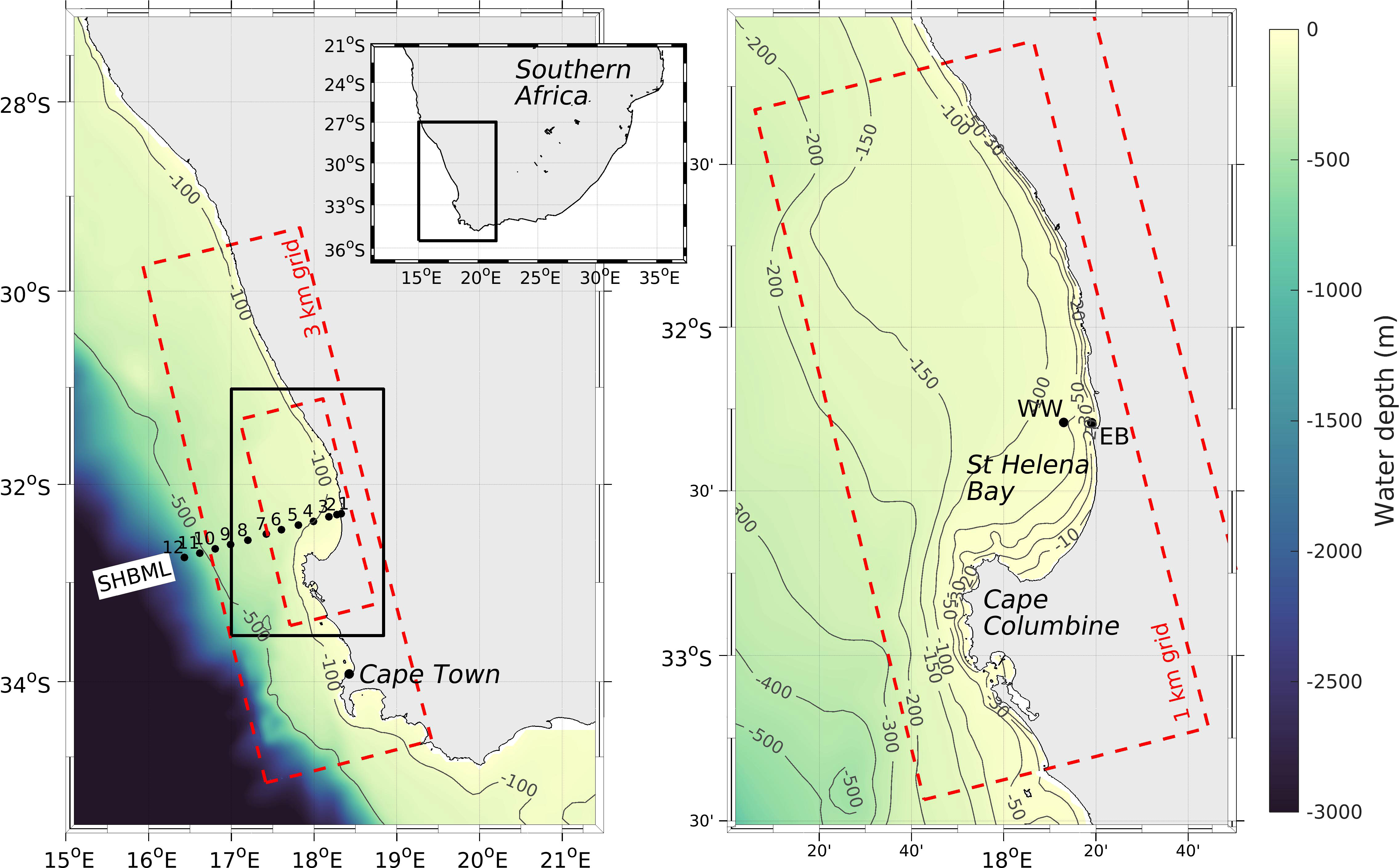
Figure 1 Locality map indicating the model grid extents, bathymetry and locations of previously published in-situ data. A 1 km resolution child domain, centred over St Helena Bay, is nested within a 3 km resolution parent domain. The shown bathymetry within the model domains is derived from digital navigation charts for the region provided by the Hydrographer of the SA Navy, while data outside the model is taken from the 30-arc second GEBCO dataset.

2 Methods

2.1 In situ data for model validation

Various in-situ datasets are presented alongside model output, with the aim of assessing the model performance at multiple time-scales, starting from seasonal climatologies.

The seasonal variability of the water column structure across the continental shelf is taken from quasi monthly Conductivity-Temperature-Depth (CTD) casts along the St Helena Bay Monitoring Line (SHBML) from March 2000 to August 2017 (Oceans and Coastal Research, 2017). The transect is comprised of twelve stations orientated approximately perpendicular to the isobaths off St Helena Bay (Figure 1). A detailed description of the data is provided in Lamont et al. (2015). Measurements from all available cruises were used to calculate monthly climatologies of temperature and salinity at each station on a 1 m vertical grid.

The inter-annual and event-scale upwelling/relaxation dynamics in the nearshore region of St Helena Bay is taken from daily averaged temperature observations from a fixed mooring in Eland’s Bay near the surface (∼5 m water depth) and at the seabed (∼20 m water depth) over the three year period from November 2008 to November 2011 (‘EB’ in Figure 1). These data are described in more detail in Pitcher et al. (2014).

The super-diurnal variability of the system is informed by concurrent deployments of Wirewalker wave-powered profilers (Rainville and Pinkel, 2001; Pinkel et al., 2011) and bottom-mounted Acoustic Doppler Current Profilers (ADCP) providing horizontal velocity components and temperature at a temporal resolution of 10 min and vertical resolutions of 1 m and 0.25 m, respectively (‘WW’ in Figure 1). The full dataset is described in detail in Lucas et al. (2014), although only data from the month of March 2011 are revisited in this study for model validation purposes. This period was specifically selected so that the model output could be compared with the reduced physics experiments of Fearon et al. (2020; 2022). The data were filtered in time to provide a two hour running mean at 30 min intervals, sufficient for analysing the super-diurnal processes of interest.

2.2 Satellite SST data

This study makes use of the Group for High Resolution Sea Surface Temperature (GHRSST) dataset for the Eastern Atlantic Region from the Spinning Enhanced Visible and InfraRed Imager (SEVIRI, https://podaac.jpl.nasa.gov/dataset/SEVIRI_SST-OSISAF-L3C-v1.0) (OSISAF, 2015). The geostationary orbit of the satellite allows data to be made available at hourly intervals from June 2004 to present, on a 0.05° regular grid. The high temporal resolution of the data is used to assess day vs night-time SST’s over the area of interest. Only data with a quality flag of 3 and greater are used in the presented analysis, as recommended in the scientific validation report for the product (SAF, 2018).

2.3 Description of the model

The ocean model employed in this study is the V1.0 official release of the Coastal and Regional Ocean COmmunity model (CROCO, http://www.croco-ocean.org/), an ocean modelling system built upon ROMS AGRIF (Shchepetkin and McWilliams, 2005). CROCO is a free-surface, terrain-following coordinate oceanic model which solves the Navier-Stokes primitive equations by following the Boussinesq and hydrostatic approximations. The model solves equations governing the conservation of horizontal momentum, hydrostatic balance, incompressibility and the conservation of tracers (temperature and salinity). A curvilinear Arakawa C-grid is used for the discretisation of the horizontal plane, while the vertical grid is discretised using a terrain-following (σ) coordinate reference system.

The choice of the vertical turbulent viscosity scheme is particularly important within the context of this study, as we attempt to highlight diapycnal mixing driven by super-diurnal wind variability. Initial simulations indicated that CROCO’s default K-profile parameterization (LMD-KPP) scheme resulted in an over-estimation of vertical mixing within the nearshore regions of St Helena Bay when compared with the observations. The results presented in this study therefore adopt the k-ϵ turbulent closure scheme within the Generic Length-Scale (GLS) formulation (Umlauf and Burchard, 2003; 2005), which provided a better fit to the observations. Horizontal eddy viscosity and diffusivity are typically ignored in regional configurations using ROMS (e.g. Marchesiello et al., 2003; Veitch et al., 2010). Instead, horizontal dissipation at the grid scale is determined by dissipation associated with a split and rotated third-order upstream biased horizontal advection scheme (Marchesiello et al., 2009). Bottom friction is parametrised using a quadratic drag law, where the bottom roughness length parameter is taken as 0.001 m. A nonlinear equation of state is used for the computation of density (Jackett and Mcdougall, 1995). The model configuration, as described below, effectively constitutes a dynamical downscaling of a global reanalysis product to ∼1 km resolution over St Helena Bay, so that the high-frequency bay-scale processes can be better assessed.

2.3.1 Discretisation

The model is comprised of a ~3 km horizontal resolution parent domain as well as a ~1 km horizontal resolution child domain, both centred around St Helena Bay and aligned according to the approximate orientation of the coastline (Figure 1). 2-way nesting is implemented between the parent and child domains, whereby at each time-step the parent domain provides boundary conditions for the child domain, which in turn provides feedback to the parent domain (Debreu et al., 2012). 50 levels are used to define the vertical grid of both domains. Baroclinic time-steps of 6 min and 2 min are adopted for the temporal integration of the parent and child domains, respectively, reflecting the factor 3 difference in the spatial resolution of the domains. 60 barotropic time-steps are computed within each baroclinic time-step.

2.3.2 Bathymetry

The bathymetry assigned to the model grids is interpolated from digital versions of the most detailed available navigation charts for the region, as provided by the Hydrographer of the South African Navy. The interpolated bathymetry is smoothed to maintain a slope parameter ($r=\frac{\nabla H}{H}$) of less than 0.25 everywhere in the domain in an attempt to circumvent the well-known horizontal pressure gradient errors associated with $\sigma$-coordinate models with steep slopes (e.g. Haney, 1991). Minimum depths of 20 m and 5 m are enforced for the parent and child domains, respectively, to avoid vertical advection errors associated with thin vertical layers in shallow water. A semi-implicit vertical advection scheme is adopted to further assist in this regard. A hyperbolic tangent function is used over the sponge layer of the parent domain (10 grid cells wide) to gradually ramp up the model bathymetry to the 30-arc second GEBCO dataset at the open boundaries of the model (Weatherall et al., 2015). This was done to match the internal bathymetry at the model boundaries with that of the global model providing lateral boundary forcing conditions (Section 2.3.4). The resulting model bathymetry is shown in Figure 1.

2.3.3 Atmospheric forcing

Atmospheric variables to force the model at the surface (10 m wind velocity components, short- and long-wave solar radiation, air temperature, relative humidity and precipitation) are taken from a Weather Research and Forecasting (WRF) model configuration developed by the Climate Systems Analysis Group (CSAG) at the University of Cape Town (UCT). The atmospheric simulation is a dynamical downscaling of the ERA-Interim global atmospheric reanalysis (https://www.ecmwf.int/en/forecasts/datasets/reanalysis-datasets/era-interim) to high resolution over southern Africa, as part of the Wind Atlas for South Africa (WASA) project (Lennard et al., 2015). The WASA model output is available on a 3 km horizontal resolution grid at hourly intervals for the period November 2005 to October 2013 (8 years). The offshore extent and orientation of our parent grid coincides with that of the 3 km resolution WRF model grid.

We use three different types of wind forcing with the aim of isolating the influence of the land-sea breeze on the dynamics of the system, as summarised in Table 1. ${\tau }^{real}$ uses bulk parameterisation (Fairall et al., 1996; 2003) for the online computation of hourly wind stress components from the WASA 10 m wind velocity components. ${\tau }^{daily}$ uses forced daily averaged wind stress components which are output from the simulation using ${\tau }^{real}$. In so doing, simulations using ${\tau }^{daily}$ maintain the identical net Ekman dynamics as simulations using ${\tau }^{real}$, while the influence of the super-diurnal winds is removed. We further perform simulations where the diurnal anticyclonic rotary component of the wind stress (${\tau }^{ac}$) is super-imposed onto ${\tau }^{daily}$, and adopt the nomenclature ${\tau }^{daily+ac}$ for this wind forcing. ${\tau }^{ac}$ is computed from consecutive 7 day windows, as described in Fearon et al. (2020), and represents the component of the winds which rotates at a diurnal frequency and in the same direction as the locally forced inertial oscillations. With this forcing we aim to excite the diurnal-inertial oscillations in response to the land-sea breeze, while excluding any additional effects induced by the super-diurnal component of the winds which may be present in ${\tau }^{real}$. All three simulations use bulk parameterisation (Fairall et al., 1996; 2003) for the online computation of hourly freshwater and heat fluxes from the WASA data.

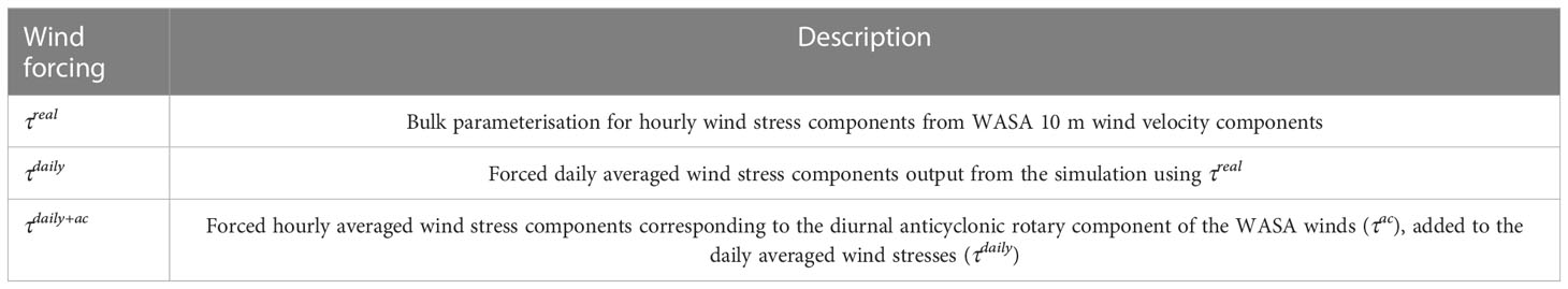
Table 1 Summary of wind forcing nomenclature adopted in this paper.

2.3.4 Lateral boundary conditions

Lateral boundary conditions for the parent domain are interpolated from daily averaged data of the ocean state (temperature, salinity, horizontal current components and surface elevation) obtained from a 1/12° global ocean reanalysis product provided by the HYCOM consortium (https://www.hycom.org/data/glbu0pt08/expt-19pt1). Following Dey et al. (2021), monthly biases in the HYCOM temperature and salinity data, computed with respect to the CSIRO Atlas of Regional Seas climatology (CARS2009, https://www.cmar.csiro.au/cars), were removed to improve model performance in the coastal region of interest. The specified water levels exclude tidal variability, which has been shown to make an insignificant contribution to current observations within St Helena Bay (Fawcett et al., 2008).

Open boundary conditions (OBCs) are implemented at the lateral boundaries of the model as described in Marchesiello et al. (2001). The model solution is ‘nudged’ to the specified boundary values using relaxation times of 1 day and 1 year for inward and outward radiation, respectively. Nudging is applied within the sponge layer of the model (10 grid cells wide) using a gradual decrease (cosine profile) from the open boundary to the inner border of the sponge layer.

2.4 Computation of climatologies

Each of the three types of wind forcing (Table 1) are used to integrate the model over the period 01 November 2005 to 31 December 2012 (7 years), spanning the duration over which all forcing data are available. Three hourly ‘snapshots’ of temperature generated over the entire simulation period are used to assess day- vs night-time sea surface temperature differences in the model. We use model output times of 14:00 and 02:00 (local time, UTC+2) for this purpose, and limit the analysis to the nominally upwelling months of October to March, which also coincides with enhanced land-sea breeze forcing in the region of interest (Fearon et al., 2020).

Daily averaged output from the 7 year simulations are used to compute climatologies of temperature and horizontal currents, allowing for an assessment of the impact of the land-sea breeze on the mean state of the vertical water column structure and circulation over the area of interest. Again, this analysis is confined to the nominally upwelling months of October to March. Upwelling and relaxation wind regimes are considered separately, as different sub-diurnal processes are at play in each. To distinguish between these regimes we consider the time-series of the 3 day average alongshore wind stress for a location in the centre of St Helena Bay, as shown in Figure 2. We take active upwelling as times where the 75^th percentile 3 day average alongshore wind stress is exceeded (i.e. the black time-series above the red line), while relaxation periods are identified as times where the 3 day average alongshore wind stress falls below the 25^th percentile value (i.e. the black time-series below the blue line). Composite means are then presented based on these wind regimes.

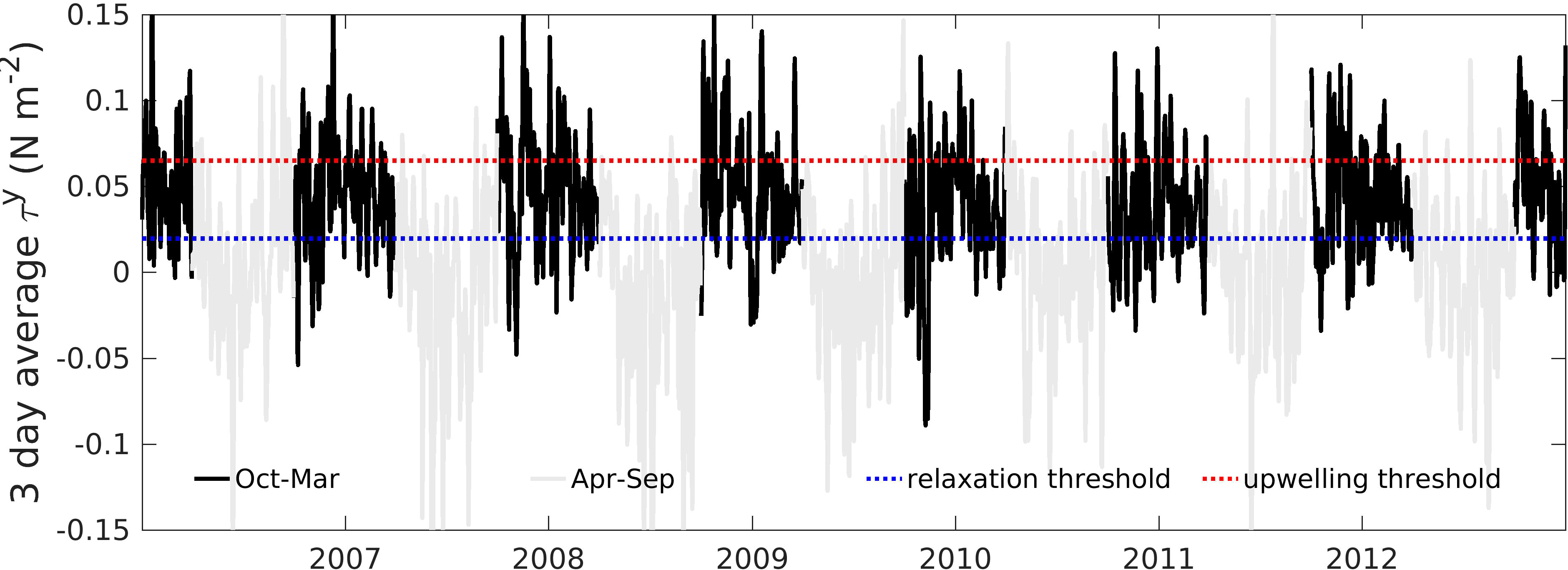
Figure 2 Time-series of 3 day average alongshore wind stress (${\tau }^y$) extracted from the model at a location in the centre of St Helena Bay (‘P’ in Figure 3). The shown relaxation and upwelling thresholds correspond to the 25^th and 75^th percentile ${\tau }^y$ for the nominally upwelling months of October-March.

2.5 Event-scale mixing experiment

Given that one of the main implications of the land-sea breeze in EBUS is its effect on vertical mixing, we present an experiment specifically designed to examine the event-scale mixing processes in the model over the weekly time-scale associated with upwelling events. To do this, we compare hourly output from two simulations, one forced by ${\tau }^{daily}$ and one forced by ${\tau }^{daily+ac}$, each initialised on 25 January 2007 from the simulation forced with ${\tau }^{daily}$ (this ensures that the influence of the land-sea breeze is absent from the initial condition in both simulations). The initialisation date was subjectively chosen to be at the end of a relaxation event during which a shallow stratified surface layer developed within St Helena Bay, as shown in Figures 3A, B. The vertical isotherms at the offshore extent of this shallow surface layer (60 to 80 km offshore) are associated with the upwelling cell off Cape Columbine, and associated equatorward flowing Columbine Jet, which represents a dynamic offshore boundary of the bay. The model is integrated over a 7 day period which is characterised by a local amplification of land-sea breeze, as indicated by the amplitude of the diurnal anticlockwise rotary component of the winds (${\tau }^{ac0}$) (Figure 3C). It is also a period of upwelling-favourable winds, as indicated by the mean wind stress (Figure 3D). Note that we use ${\tau }^{ac0}$ to refer to the amplitude of the rotating wind stress component, while ${\tau }^{ac}$ denotes the rotating wind stress vector. Figure 3E provides the time-series of wind stress components for ${\tau }^{daily}$ and ${\tau }^{daily+ac}$ for a location in the centre of St Helena Bay.

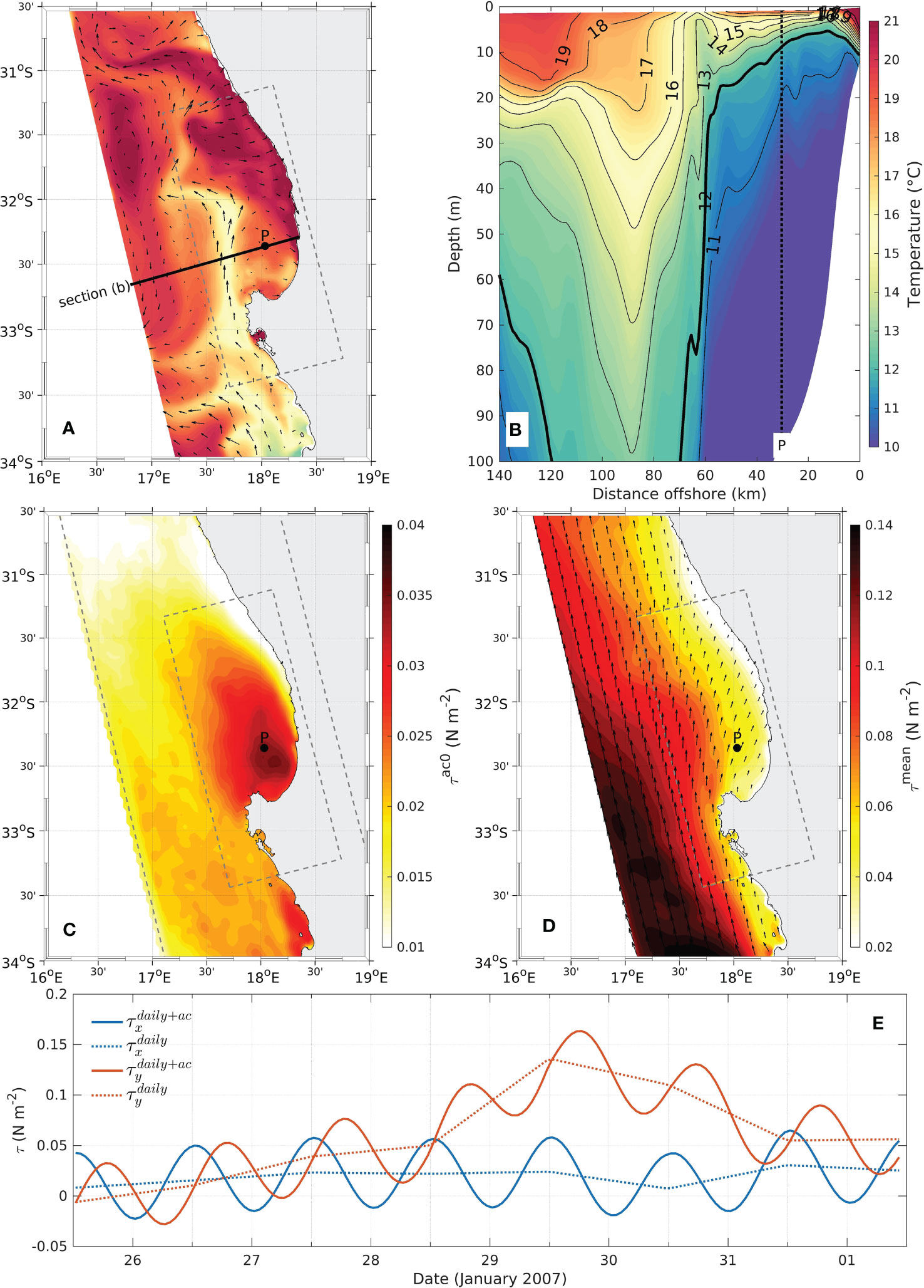
Figure 3 Initial temperature condition and wind stress forcing for 7 day experiments initialised on 25 January 2007 from the model forced with ${\tau }^{daily}$. (A) Mean sea surface temperature. (B) Mean vertical section of temperature across the model domain over the upper 100 m of the water column. (C) Amplitude of the diurnal anticlockwise rotary component of the wind stress (${\tau }^{ac0}$) over the 7 day duration of the experiment. (D) Mean wind stress (${\tau }^{mean}$) over the 7 day duration of the experiment. (E) Time-series of wind stress components for ${\tau }^{daily}$ and ${\tau }^{daily+ac}$ at Station ‘P’, in the centre of St Helena Bay.

The analysis of diapycnal mixing in the model is aided by initialising the model with a subsurface passive tracer ($C$, in arbitrary tracer units per volume, ATU m^-3). $C$ is initialised to a value of 1 for temperatures of 12°C and less, 0 for temperatures of 13°C and above, while linear interpolation is applied for temperatures between 12°C and 13°C. This approach is also adopted for specifying the passive tracer at the lateral boundaries of the model. The cumulative diapycnal mixing in the model is quantified by integrating the passive tracer from the depth of the 12°C isotherm to the surface:

It is informative to isolate the effect of the land-sea breeze forcing on $C_s$, which is done by computing the difference in $C_s$ for simulations which both include and exclude the diurnal anticlockwise rotary component of the wind stress (${\tau }^{ac}$):

$\text{Δ}{C}_s$ therefore represents a diagnostic aimed at highlighting the increase in cumulative diapycnal mixing due to the inclusion of land-sea breeze forcing.

We further use the vertical displacement of the 12°C isotherm to diagnose internal wave generation and propagation in the model due to the inclusion of land-sea breeze forcing. To this end, the depth of the 12C isotherm is presented as the displacement from the daily running average, allowing us to isolate the super-diurnal variability induced by the applied land-sea breeze forcing.

3 Results

3.1 Model validation

The purpose of the model validation is to assess the skill of the model at representing the variability of the system at multiple time-scales, including seasonal fluctuations (Figure 4), upwelling/relaxation events (Figure 5), and higher frequency process associated with the land-sea breeze (Figure 6). Preference is given to in-situ data over satellite observations for the model validation owing to the nearshore and high-frequency nature of the processes of interest.

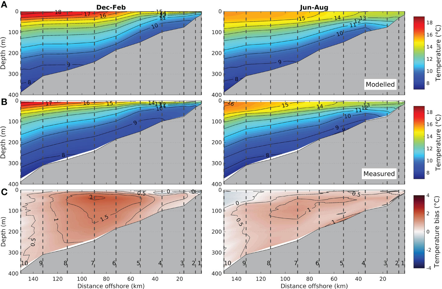
Figure 4 Seasonal temperature climatologies for the St Helena Bay Monitoring Line (SHBML) as computed from the model (A), from the observations (B) and the resulting model bias (C). The numbered vertical dashed lines denote the station locations shown in Figure 1.

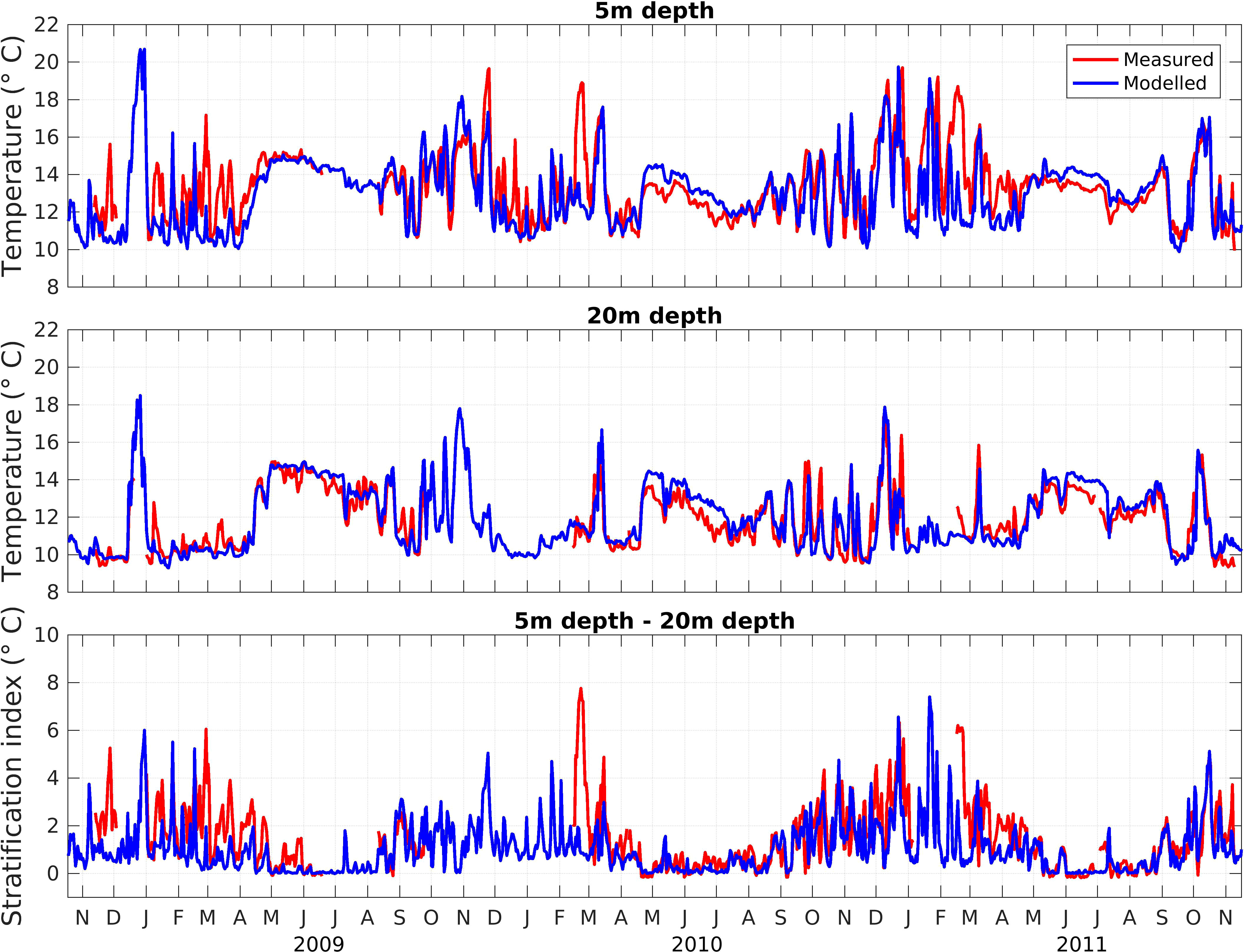
Figure 5 Time-series comparison of daily averaged measured and modelled temperature at 5 m and 20 m depths at the Elands Bay fixed mooring (‘EB’ in Figure 1), located in 20 m water depth). The stratification index is simply the difference between the temperature at 5 m and 20 m depths.

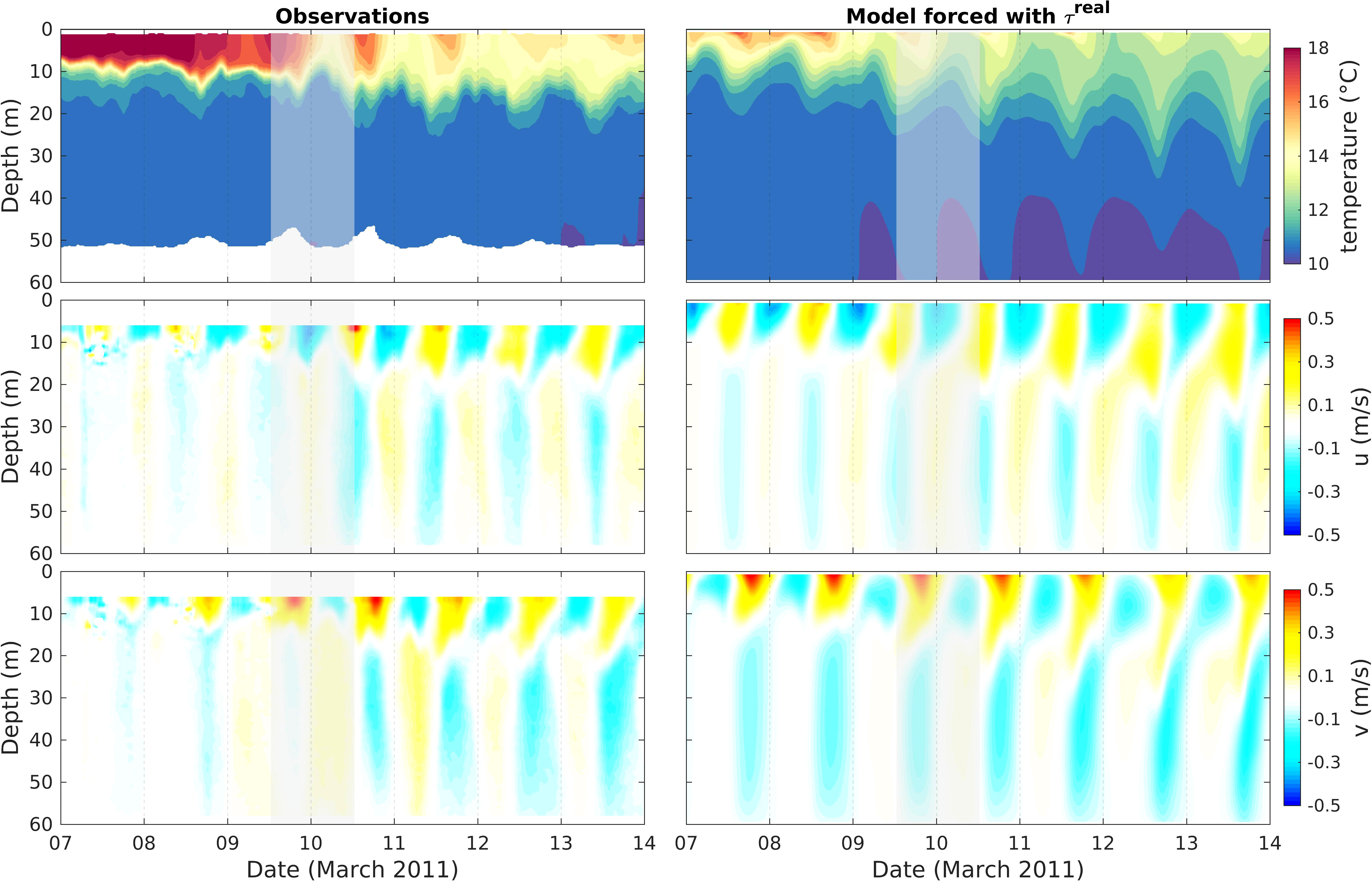
Figure 6 Observed (left) and modelled (right) temperature and horizontal velocity components over an upwelling event accompanied by diapycnal mixing at the Wirewalker fixed mooring in 60 m water depth (‘WW’ in Figure 1). The shaded time denotes the period considered in Figure 7.

Figure 4 presents a comparison of modelled and observed seasonal temperature climatologies along the St Helena Bay Monitoring Line (‘SHBML’ in Figure 1). The vertical water column characteristics for the offshore region (Station 7 and offshore) is shown to be distinct from those in the nearshore waters of St Helena Bay (Stations 1 to 4). During austral summer (December to February), Stations 3 and 4 (in the middle of St Helena Bay) are characterised by a highly stratified shallow surface layer overlaying cool subsurface waters. In contrast, winter months at these stations are characterised by a nearly fully mixed water column. Nearshore temperatures are on average cooler than those offshore, particularly during summer, in line with the seasonal variability in upwelling-favourable winds. The climatological model bias within St Helena Bay (Stations 1 to 4) is below 1°C for both summer and winter seasons, indicating that the seasonal variability in the mean state of water column over the area of interest is well represented in the model.

Figure 5 presents a 3 year time-series of measured and modelled daily averaged temperature at the Elands Bay fixed mooring (‘EB’ in Figure 1), while summary statistics for the nominally winter (April-September) and summer (October-March) periods are provided in the Supplementary Table S1. The data indicate a well-mixed water column during winter with relatively little variability, while summer reflects the variability associated with upwelling/relaxation events. Extended periods of upwelling result in a drop in temperature in both surface and subsurface waters, while relaxation of equatorward winds drive stratification events through the warming of surface waters which are advected inshore and poleward (Fawcett et al., 2007; Fawcett et al., 2008; Pitcher et al., 2014). Relaxation events can lead to the subduction of warm water to the bottom, as reflected in the time-series at 20 m depth. The model is shown to under-predict surface warming for some relaxation events (top panel of Figure 5), suggesting that the surface heat flux and/or the inshore and poleward advection of heat is not adequately captured for these events. This results in a cool bias of ~1.2C in the surface waters during summer. Surface model temperatures achieve correlation coefficients of 0.8 and 0.92 for the summer and winter periods, respectively. Subsurface bias is low throughout the year (<0.6C) with correlation coefficients of 0.88 and 0.89 for the summer and winter periods, respectively. Overall, these results indicate that the model shows acceptable skill at capturing the salient features of the upwelling/relaxation dynamics in the nearshore waters of St Helena Bay.

For reference, Supplementary Table S2 provides summary statistics at the Elands Bay mooring, but for the simulation forced with daily averaged wind stress (${\tau }^{daily}$). The statistics confirm that the model performance is significantly reduced when the super-diurnal winds are excluded in the model forcing. For example, the correlation coefficient for surface temperature reduces from 0.8 to 0.68 during summer, and from 0.92 to 0.83 during winter, highlighting the importance of super-diurnal winds in representing upwelling-relaxation dynamics in the model.

We now further analyse the extent to which the observed super-diurnal variability, embedded within the sub-diurnal upwelling dynamics, is captured by the model forced with ${\tau }^{real}$. Figure 6 presents the temporal evolution of temperature and horizontal velocity components through the water column for a 7 day period at the Wirewalker mooring in 60 m water depth (‘WW’ in Figure 1), both in the observations and in hourly output from the model. For reference, this is the same 7 day period considered in the reduced physics experiments of Fearon et al. (2020; 2022). A time-series of wind stress components over this time period at the Wirewalker location can be found in Figure 2 of Fearon et al. (2022). The considered period begins with a relaxation event characterised by a highly stratified two layer system. The onset of an upwelling event is shown to be accompanied by strong variability at the diurnal-inertial frequency in both the temperature and horizontal velocity profiles, with a 180° phase shift between the surface and subsurface currents. The model performance over the full month of March 2011 is summarised in the Supplementary Figure S1. Modelled temperatures are shown to be under-estimated near the surface, although here temperature correlation is highest (∼0.8 in the surface layer of the model), reflecting general agreement in the super-diurnal variability in surface temperature. Correlation coefficients of 0.4-0.6 and 0.6-0.7 are attained for near-bottom and near-surface current velocities, respectively. Overall, the comparison indicates agreement between the modelled and observed super-diurnal variability, and provides some confidence that the model can be used to gain further insight into the spatial and temporal variability of the processes of interest.

3.2 Super-diurnal effects of the land-sea breeze

The shaded time in Figure 6 denotes a 24 hour period characterised by the onset of strong diurnal variability in surface temperature, both in the observations and in the model. The evolution of the spatial variability in sea surface temperature (SST) and surface currents over St Helena Bay for this 24 hour period is further assessed in Figure 7. It is worth noting that the shown period displays some typical features of the region, as documented in the literature. For instance, upwelling along the coastline south of St Helena Bay sets up a shelf edge front and the associated Goodhope Jet, a strong equatorward current in geostrophic balance with the cross-shore pressure gradient (Strub et al., 1998; Veitch et al., 2018). North of Cape Columbine, the Goodhope Jet tends to bifurcate due to shelf widening, resulting in offshore and alongshore components (Shannon and Nelson, 1996; Veitch et al., 2018), the latter corresponding to the Columbine Jet which effectively defines a dynamic boundary between the nearshore waters of St Helena Bay and those offshore (Lamont et al., 2015). Also evident in the model is upwelling along a narrow belt on the eastern periphery of the bay and the formation of an inner shelf upwelling front (Jury, 1985; Taunton-Clark, 1985). Mean surface flow on the inner shelf during active upwelling is typically equatorward, in agreement with observations (Fawcett et al., 2008).

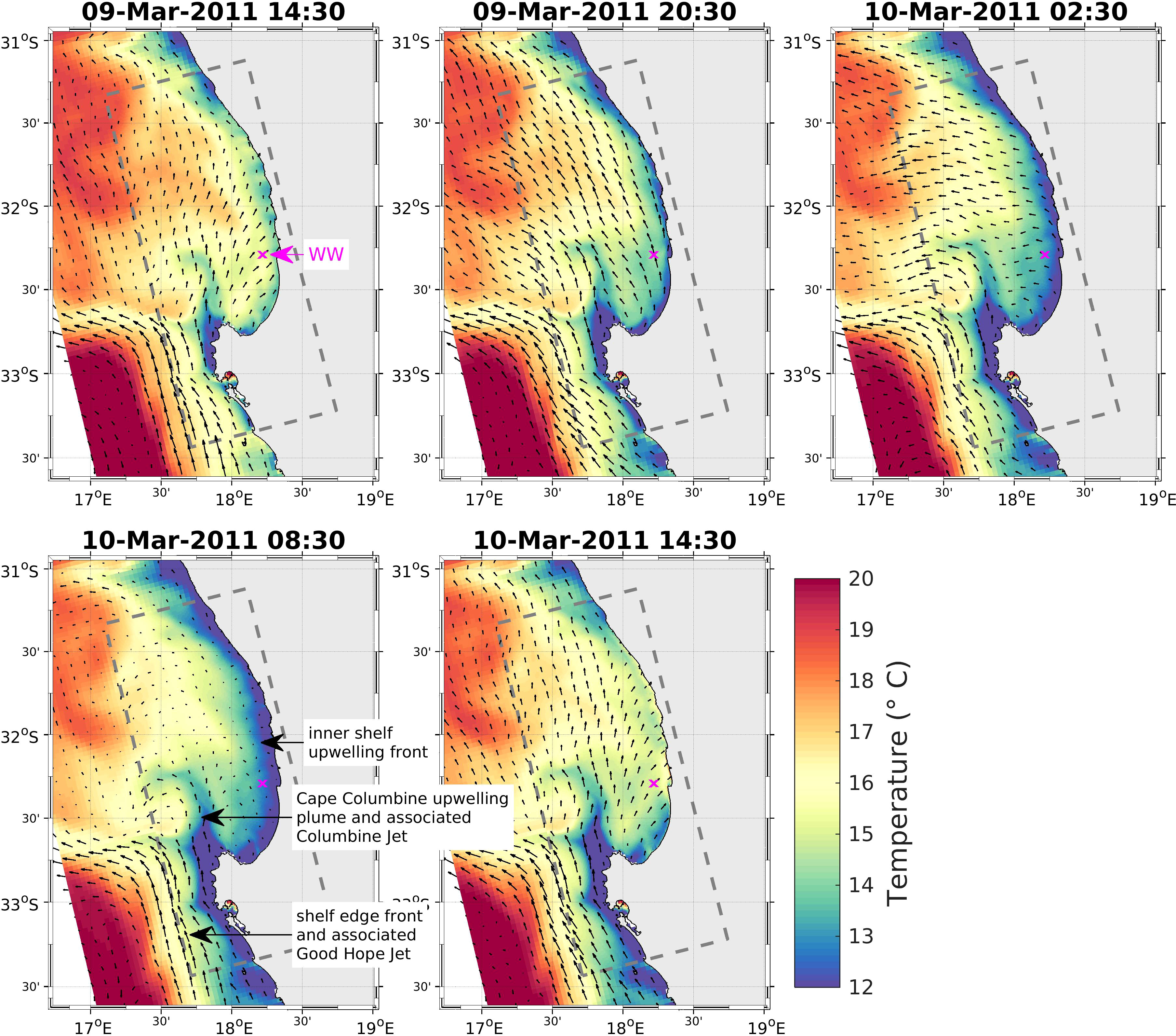
Figure 7 6 hourly snapshots of modelled SST and surface current vectors over an upwelling event, demonstrating the outcropping and subduction of the inner shelf upwelling front over a day in response to inertial motions. The Wirewalker observations (denoted by the magenta cross) capture the strong diurnal variability in SST, as shown in Figure 6. Times are local time, UTC+2.

Figure 7 highlights the super-diurnal variability in surface currents and temperature embedded within these features, particularly within St Helena Bay. Here, the oscillatory nature of the surface currents is clearly evident, whereby the cross-shore component in the surface current is offshore at night, turning to onshore during the day. This phasing is tied to that of the land-sea breeze, indicating they are driven primarily by the diurnal-inertial resonance phenomenon. The surface currents drive the outcropping of the inner shelf upwelling front within St Helena Bay during the night (e.g. refer to the 08:30 time-step), however six hours later the newly upwelled waters are once again subducted by onshore surface currents. These processes contribute to temperature variability of greater than 5°C within the inner shelf regions of St Helena Bay over the considered 24 hour period.

Given this stark difference between day- and night-time surface temperature for this particular 24 hour period, it is prudent to assess the persistence of this effect. This is achieved by computing day- and night-time climatologies of SST, considering only the nominally upwelling months of October to March. Figure 8 presents this analysis for the GHRSST-SEVIRI satellite data over the 7 year duration of the model integration, while that of the realistically forced model is presented in Figure 9. The satellite data confirm that indeed the observed day-time SST’s are on average warmer than those at night, and that the effect increases towards the coast, where the difference exceeds 1°C (Figure 8C). A similar pattern is seen in the model, although the effect is more exaggerated, particularly in the nearshore region of St Helena Bay where the mean day-night difference in SST exceeds 2°C over much of the bay (Figure 9C). SST’s are also notably higher in the satellite data than in the model (Figures 8A, B vs Figures 9A, B). It should however be noted that flagging techniques used to ‘de-cloud’ thermal infrared satellite data are known to contribute to large warm biases in upwelling systems by attributing cold upwelled water as missing data (Dufois et al., 2012; Smit et al., 2013; Meneghesso et al., 2020; Carr et al., 2021). Our high frequency model output is therefore seen as a preferred reference for assessing diurnal variability in SST’s over the area of interest.

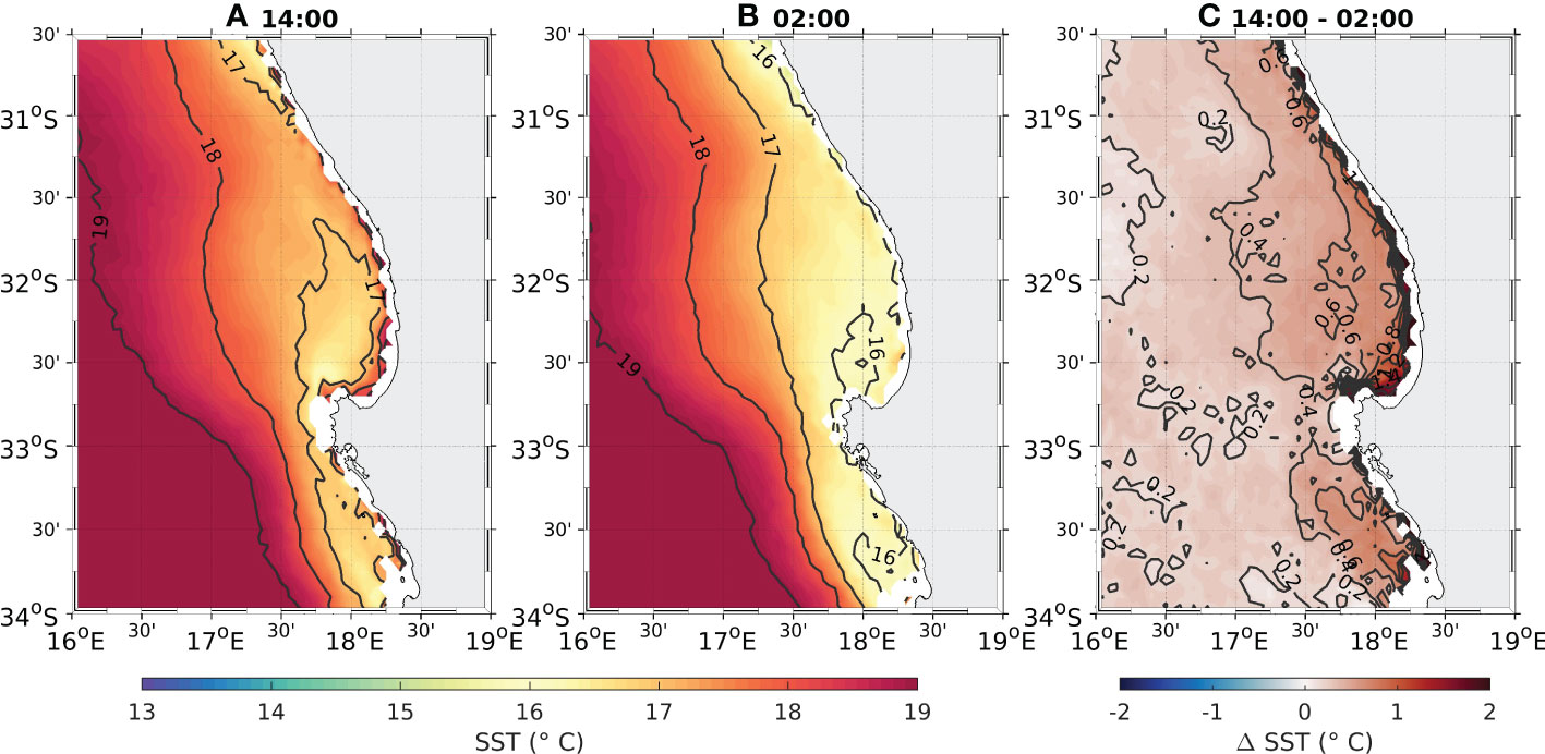
Figure 8 Day- and night-time climatologies of SST derived from GHRSST-SEVIRI satellite data for the ‘upwelling’ months of October-March. (A) Climatology computed from data at 14:00. (B) Climatology computed from data at 02:00. (C) The difference between climatologies computed at 14:00 and 02:00. Times are local time, UTC+2.

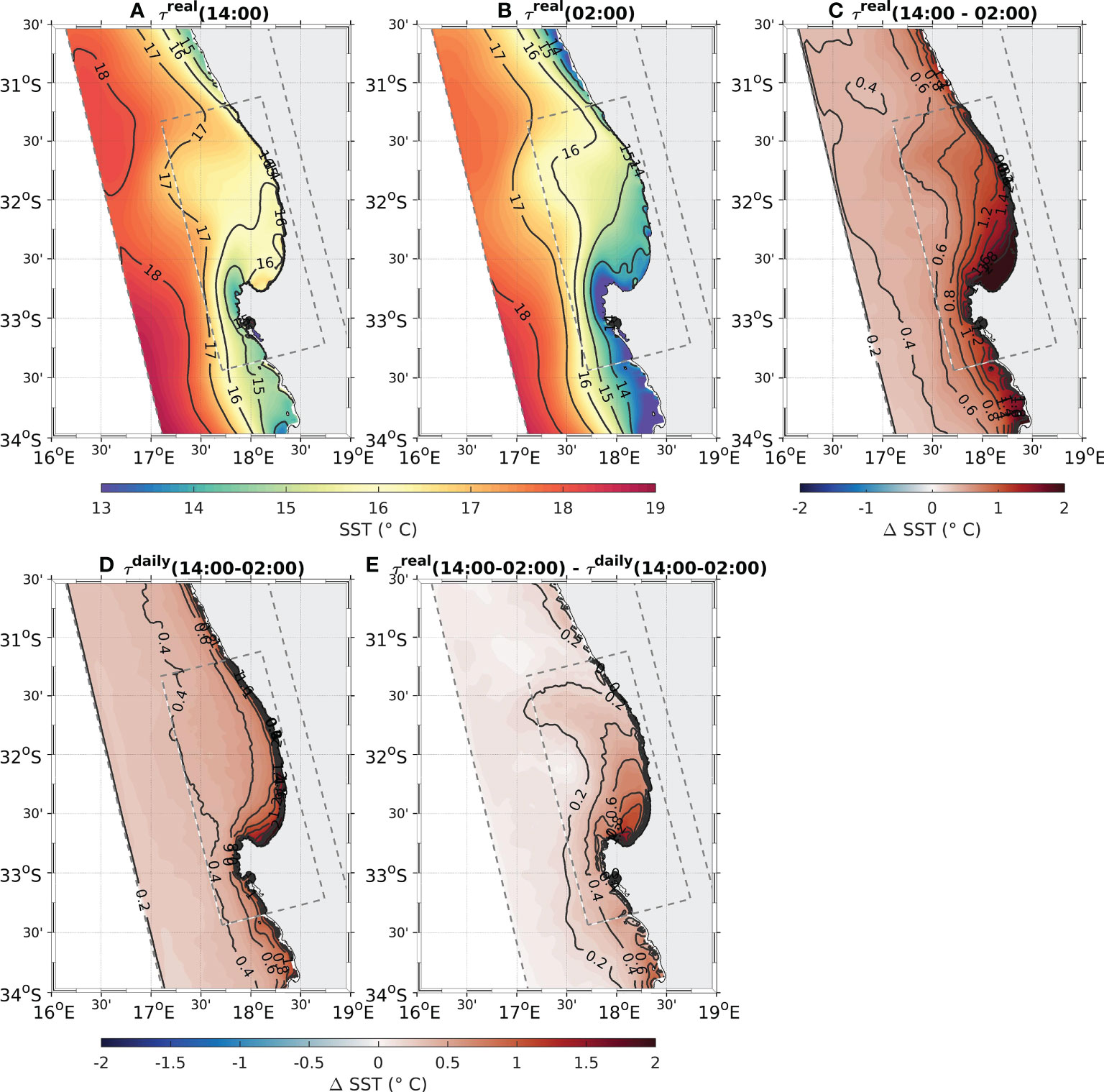
Figure 9 Day- and night-time climatologies of modelled SST for the ‘upwelling’ months of October-March. (A) SST climatology at 14:00 from the model forced by ${\tau }^{real}$. (B) SST climatology at 02:00 from the model forced by ${\tau }^{real}$. (C) Difference in day- and night-time SST climatologies from the model forced by ${\tau }^{real}$. (D) Difference in day- and night-time SST climatologies from the model forced by ${\tau }^{daily}$. (E) C - D, isolating the effect of the super-diurnal component of the winds on day- and night-time SST climatologies. Times are local time, UTC+2.

Although a strong day-night signal is evident in Figure 9C, it isn’t clear how much of this signal is due to the movement of the front by the diurnal-inertial oscillations versus surface heat fluxes driven by solar irradiance (the land-sea breeze is itself a product of diurnal heating/cooling over the land and ocean). To distil these two effects we make use of the 7 year simulation forced with τ^daily (Table 1), which maintains hourly heat fluxes but removes the diurnal-inertial oscillations. The mean day-night difference in SST for this simulation is shown in Figure 9D, while the effect of the diurnal-inertial oscillations is estimated by subtracting this from the overall signal (Figure 9E). The influence of the land-sea breeze on the diurnal fluctuations in SST is shown to be particularly enhanced in the nearshore region of St Helena Bay, where the mean difference exceeds 1°C. Diurnal warming due to solar irradiance is also enhanced in the southern extent of the bay, leading to a pronounced combined effect.

3.3 Event-scale diapycnal mixing

One of the main implications of the high amplitude diurnal-inertial oscillations is their impact on vertical mixing. We now present the results from an experiment specifically designed to examine these processes over an upwelling event accompanied by an enhanced land-sea breeze (refer to Section 2.5 for the experiment setup). Figure 10 shows the temporal evolution of the cross-shore component of velocity and the passive tracer at a location in the centre of St Helena Bay (‘P’ in Figure 3). The comparison of the simulations forced with both ${\tau }^{daily+ac}$ (left panels) and ${\tau }^{daily}$ (right panels) clearly demonstrates how the inclusion of ${\tau }^{ac}$ leads to shear-driven deepening of the thermocline primarily in response to the diurnal-inertial resonance phenomenon and the associated injection of subsurface waters into the surface layer, all of which are embedded in the sub-diurnal upwelling dynamics.

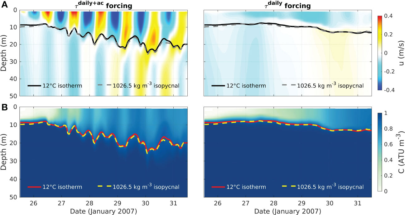
Figure 10 Temporal evolution of the model solution for the cross-shore component of velocity (A) and the passive tracer (B) over the upper 50 m of the water column at a location in the centre of St Helena Bay (‘P’ in Figures 3, 12). The model is initialised on 25 January 2007 (Figure 3) and forced with both ${\tau }^{daily+ac}$ (left panels) and ${\tau }^{daily}$ (right panels).

Figure 10 also indicates the depth of the 12°C isotherm, which reveals a complex pattern of thermocline displacements when land-sea breeze forcing is included in the model. These thermocline displacements can be interpreted from the Hovmöller diagram shown in Figure 11A. The model reveals how the super-diurnal onshore and offshore advection of the surface layer generates large thermocline displacements at both the landward and offshore extents of the bay. Offshore surface flow is associated with upward thermocline displacements at the land boundary and downward thermocline displacements at the offshore extent of the bay, and vice versa for onshore surface flow. These forced diurnal vertical motions trigger offshore and onshore propagating internal waves which are evanescent, given that the latitude is poleward of 30°S (Zhang et al., 2010). In addition to the expected thermocline pumping and internal wave generation at the land boundary (Millot and Crepon, 1981; Fearon et al., 2022), the results point to an additional offshore source of internal wave generation associated with the Cape Columbine upwelling plume, where thermocline pumping is in fact larger than at the land boundary. This is attributed largely to the spatial heterogeneity in the depth of the Ekman layer which changes abruptly at the upwelling plume (see Figure 3B) and introduces large spatial variability in the forced diurnal-inertial surface currents. Enhanced vorticity associated with the alongshore jet would further serve to introduce spatial variability in the diurnal-inertial motions in this region (Weller, 1982; Klein et al., 2004; Elipot et al., 2010). The spatial variability in the forced diurnal-inertial oscillations drive convergences and divergences in the surface flow which are responsible for the thermocline pumping and internal waves seen in the model.

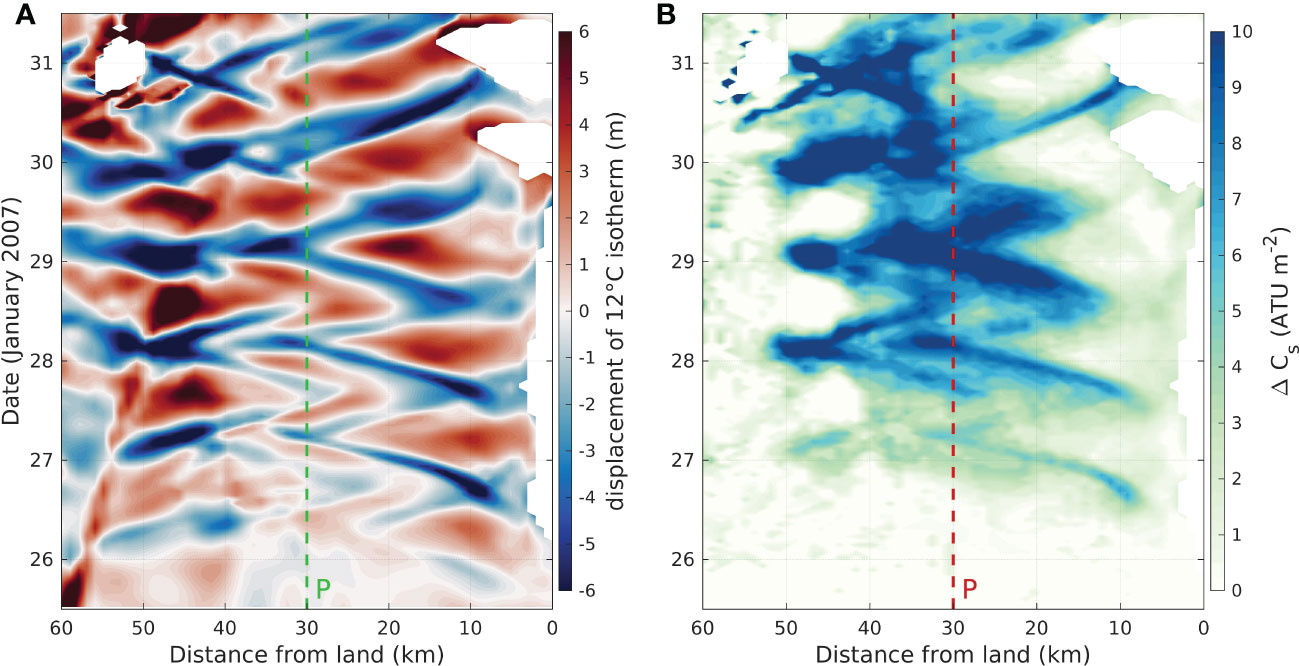
Figure 11 (A) Hovmöller diagram of the displacement of the 12°C isotherm from the daily running average isotherm for the model forced with ${\tau }^{daily+ac}$. Blue (red) denotes downward (upward) displacement of the thermocline. (B) Hovmöller diagram of the increase in the passive tracer integrated from the 12°C isotherm to the surface ($C_s$) due to the inclusion of ${\tau }^{ac}$ (refer to Equation 2). The initial condition for both simulations is shown in Figure 3. The section used to compute the Hovmöller diagrams is shown in Figure 12. The missing data in the model output corresponds to the outcropping of the 12C isotherm.

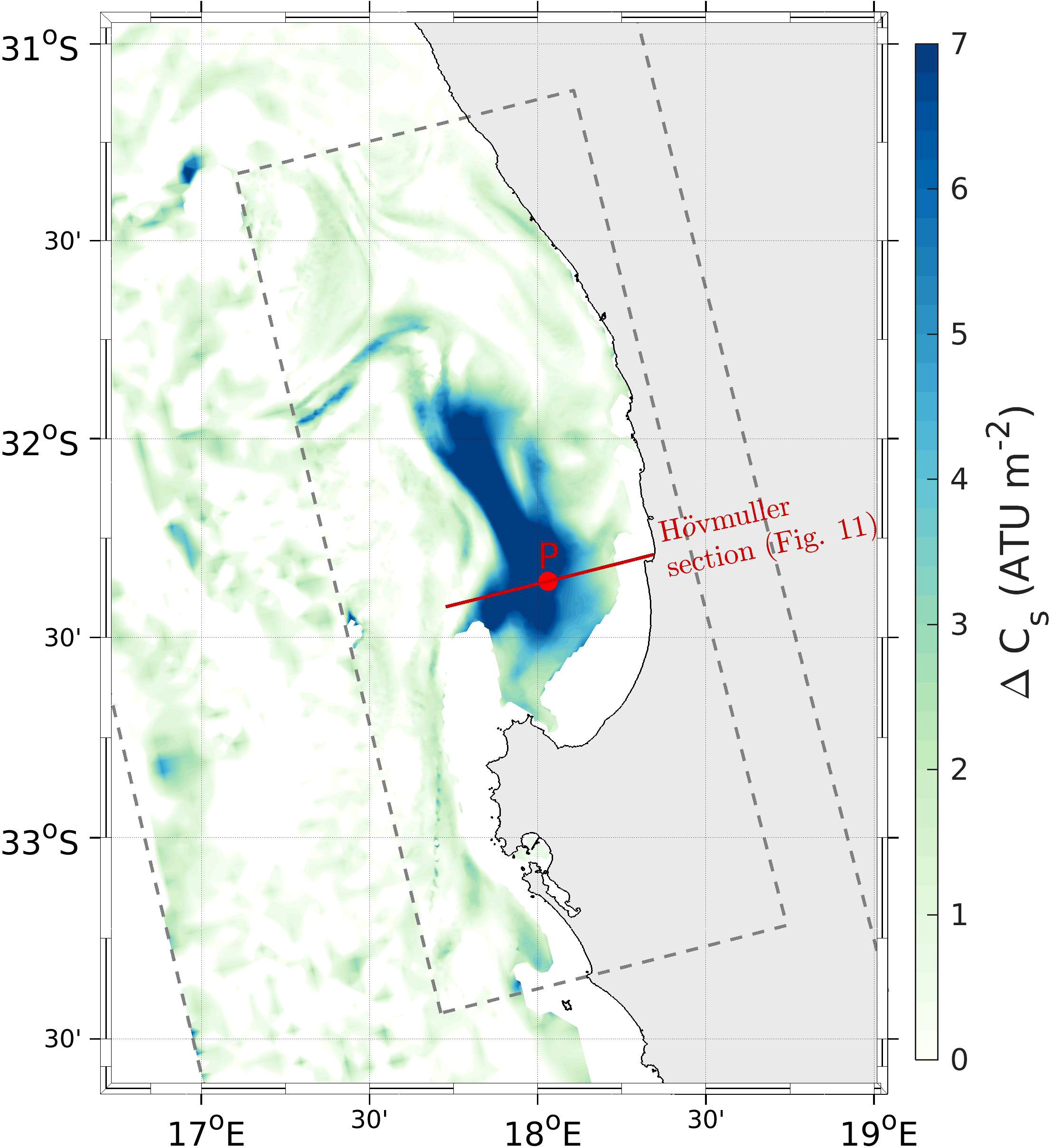
Figure 12 Increase in the passive tracer integrated from the 12°C isotherm to the surface ($C_s$) due to the inclusion of ${\tau }^{ac}$, averaged over the fifth day of the simulation (refer to Equation 2). The missing data in the model output corresponds to the outcropping of the 12°C isotherm.

Figure 11B illustrates the development of enhanced diapycnal mixing across St Helena Bay due to the inclusion of super-diurnal winds (refer to Equation 2 for how this diagnostic is computed). We note that the relative contribution of the locally forced oscillations and the evanescent internal waves on the cumulative diapycnal mixing can be difficult to separate, although we would expect mixing to be largely driven by the locally forced oscillations, while the internal waves are expected to play a secondary role (Fearon et al., 2022). The region of maximum enhanced diapycnal mixing is shown to be associated with the shallow stratified surface layer within St Helena Bay. Within this region, the cumulative diapycnal mixing varies considerably at time-scales of less than a day, in response to the onshore and offshore advection of the surface layer, and the large thermocline displacements. Regions of the largest enhancement of cumulative diapycnal mixing are typically associated with large downward thermocline displacements, given that $C_s$ represents the integration of $C$ from the 12°C isotherm to the surface. This super-diurnal variability is embedded within the sub-diurnal offshore advection of the region of maximum enhanced mixing associated with the surface layer. The spatial variability in enhanced diapycnal mixing is further explored in Figure 12, which presents the increase in $C_s$ due to the inclusion of land-sea breeze forcing, averaged over the fifth day of the simulation (29-30 January 2007). The analysis clearly identifies a region of particularly enhanced diapycnal mixing relative to the surrounding areas, associated with the shallow surface layer which had formed within St Helena Bay (Figure 3).

3.4 Sub-diurnal effects of the land-sea breeze

We now consider how the presented super-diurnal processes may affect the mean state of the vertical water column structure and circulation over the area of interest. This is achieved by comparing 7 year climatologies for simulations forced with ${\tau }^{daily}$ and ${\tau }^{daily+ac}$, thereby isolating the effect of the diurnal anticlockwise rotary component of the wind stress (${\tau }^{ac}$) (Table 1). Climatological comparisons are provided in Figures 13, 14 for upwelling and relaxation wind regimes, respectively (refer to Section 2.4 for how upwelling and relaxation wind regimes are defined for this analysis).

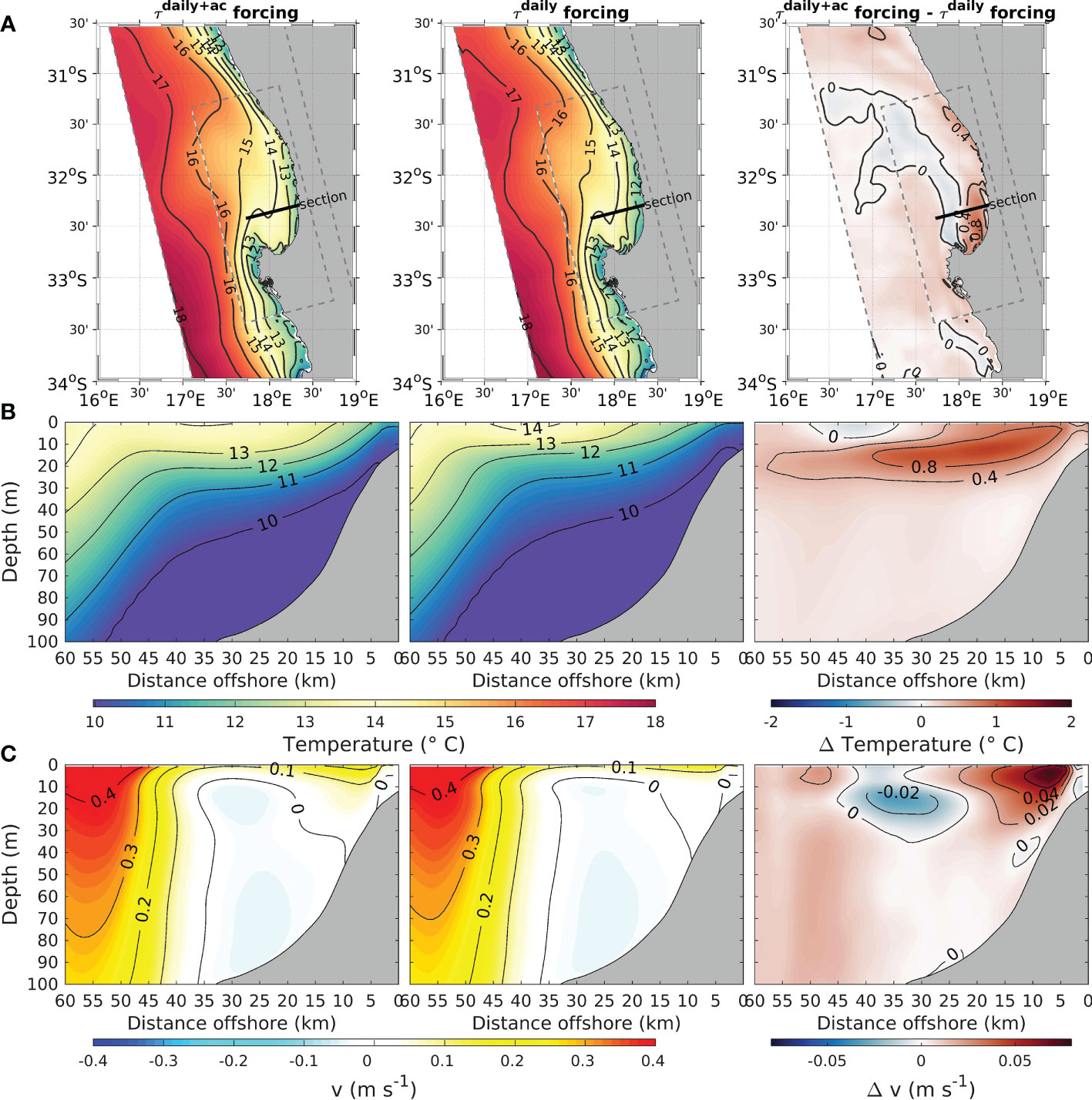
Figure 13 Impact of the diurnal anticlockwise rotary component of the wind stress (${\tau }^{ac}$) on the mean temperature and alongshore currents during upwelling conditions. The left panels show results for the simulation forced with ${\tau }^{daily+ac}$, the middle panels show results for the simulation forced with ${\tau }^{daily}$, while the right panels show the difference between the two, highlighting the impact of ${\tau }^{ac}$. (A) Climatology of SST. (B) Climatology of temperature for a vertical section through St Helena Bay (the location of the section is shown in a). (C) Climatology of the equatorward (i.e. alongshore) component of horizontal velocity ($v$) for a vertical section through St Helena Bay.

The inclusion of ${\tau }^{ac}$ during upwelling conditions is shown to drive a notable deepening of the thermocline within St Helena Bay (Figure 13B), consistent with the effects of enhanced vertical mixing driven by the diurnal-inertial oscillations. For example, at an offshore distance of 30 km, the mean 12°C isotherm depth is ~14 m for the simulation forced with ${\tau }^{daily}$, increasing to a depth of ~21 m for the simulation forced with ${\tau }^{daily+ac}$. The net warming of the entire water column in the inner shelf region (right panel of Figure 13B) however points to effects which can’t be explained purely by the vertical exchange of surface and subsurface waters. Fearon et al. (2022) used a 2D model to show how a deepened thermocline leads to a reduction in the offshore advection of the surface layer, thereby maintaining the upwelling front closer to the coast and driving a net warming of nearshore waters. This is invoked as an explanation for the nearshore warming seen in the 3D model during upwelling conditions.

Figure 13C reveals mean alongshore currents which are largely geostrophically driven, considering the cross-shore structure of the isotherms (Figure 13B). The strong equatorward current offshore of St Helena Bay (mean surface current >0.4 m s^-1 at an offshore distance of ~55 km) corresponds to the Columbine Jet, in geostrophic balance with the cross-shore pressure gradient set up by the Columbine upwelling plume. The model also indicates an equatorward mean flow associated with the inner shelf upwelling front (<~15 km offshore), in agreement with observations (Fawcett et al., 2008), while a poleward mean flow is associated with the offshore extent of the shallow surface layer inside St Helena Bay (refer to depths of ~10-30 m and offshore distances of ~20-35 km). Mean near-bottom currents within St Helena Bay are shown to be poleward, which may in part be linked to barotropic continental shelf waves (Holden, 1987), cyclonic barotropic flow in the lee of Cape Columbine (Penven et al., 2000), and negative wind stress curl through the Sverdrup relation (Veitch et al., 2010). The inclusion of land-sea breeze forcing (${\tau }^{ac}$) is shown to amplify the geostrophically driven alongshore currents associated with either end of the shallow surface layer within St Helena Bay. For example, the mean equatorward currents associated with the inner shelf upwelling front are roughly doubled in the area of maximum impact, increasing from 0.09 m s^-1 to 0.17 m s^-1 (right panel of Figure 13C). The mean poleward flow at the offshore end of the surface layer increases from 0.02 m s^-1 to 0.05 m s^-1 in the area of maximum impact. These impacts are consistent with a locally deepened thermocline, which serves to steepen cross-shore pressure gradients and therefore alongshore geostrophic flow.

During periods of wind relaxation, the inclusion of land-sea breeze forcing (${\tau }^{ac}$) is shown to drive cooler SST’s over most of the model domain (right panel of Figure 14A). This effect is particularly evident within the nearshore regions of St Helena Bay, where the mean difference between the two simulations exceeds 2°C. Inspection of the vertical water column structure (Figure 14B) reveals that the lower SST’s driven by ${\tau }^{ac}$ are compensated by warmer subsurface waters due to a deeper thermocline, consistent with the effects of enhanced diapycnal mixing by the diurnal-inertial oscillations. It is interesting to note that the net warming of the nearshore water column in response to ${\tau }^{ac}$ during upwelling periods (Figure 13B) is not at all present during periods of relaxation. This further supports the suggested mechanism for the net warming to be linked to reduced offshore advection of the surface layer, which would be largely absent during relaxation of equatorward winds.

Figure 14 As per Figure 13 but for relaxation conditions.

Periods of wind relaxation are associated with a weakened Columbine Jet, and a poleward mean flow within St Helena Bay, again consistent with inner shelf observations (Fawcett et al., 2008). During these periods, the only notable impact of ${\tau }^{ac}$ on the mean flow is again on the inner shelf, where a geostrophically driven poleward flow is associated with the subduction of the thermocline. In this case, the deepened thermocline due to the inclusion of ${\tau }^{ac}$ serves to reduce the cross-shore pressure gradients and weakens this poleward flow.

4 Discussion and conclusions

We have used a validated 3D model of the southern Benguela upwelling system to explore the influence of the land-sea breeze on temperature and current variability of the system across multiple time-scales. An over-arching finding, common to all of the presented analyses, is that the effects of land-sea breeze forcing are particularly enhanced within the inner shelf region of St Helena Bay, which is also the most productive region in the southern Benguela (Weeks et al., 2006; Demarcq et al., 2007). This is consistent with previous observational studies which have noted the ubiquitous presence of diurnal-inertial current variability in the nearshore regions of the bay (Fawcett et al., 2008; Lucas et al., 2014). Fearon et al. (2020) hypothesised that St Helena Bay possesses a combination of three physical characteristics which might promote a locally enhanced forced response to the land-sea breeze. Firstly, the bay is at a latitude of ∼32.5°S (inertial period of ∼22 hr), allowing for near-resonance between the diurnal periodicity of the land-sea breeze and the inertial response of the ocean. Secondly, the diurnal anticyclonic rotary component of the winds, which can be used as a first order estimate of the forced diurnal-inertial currents (Fearon et al., 2020), is locally enhanced over St Helena Bay. This is evident in the wind forcing over our event-scale mixing experiment (Figure 3) as well as from a seasonal climatology of this variable (Fearon et al., 2020). Thirdly, the well-known retentive circulation within the bay allows for the local development of a shallow stratified surface layer, which results in water masses which are distinct from those offshore (Lamont et al., 2015). This is an important consideration in the context of this study, as shallower surface layers are associated with larger amplitude diurnal-inertial oscillations and enhanced mixing. The confluence of these physical attributes are invoked as an explanation for the intensification of land-sea breeze-driven effects within St Helena Bay, as observed in the model.

An important finding from the model is the extent to which day- vs night-time sea surface temperatures (SST’s) vary over the model domain. The effect is again particularly stark within St Helena Bay, where modelled mean day-time SST’s are more than 2°C warmer than those at night over the nominally upwelling months of October to March. Diurnal solar irradiance does indeed contribute to this signal, particularly during conditions of low winds and high solar irradiance (Stuart-Menteth et al., 2003), however the model indicates that within St Helena Bay more than half of the signal can be attributed to the horizontal advection of strong SST gradients by diurnal-inertial surface oscillations forced by the land-sea breeze (Figure 9E). This reveals a picture of strong super-diurnal advection of water masses within the bay, which may pose challenges for observation systems in the region. In-situ observations aimed at understanding the physical and biological functioning of the system rarely capture this high-frequency variability; the observations of (Lucas et al., 2014) being a notable exception. For example, daily in-situ observations of coastal seawater temperature have provided a useful basis for computing monthly coastal temperature climatologies along the entire South African coastline (Smit et al., 2013). Our results however suggest that the time of day of these observations could play a large role in the outcome of the analysis and should be considered if the data are to be used as a ground truth for mean coastal SST’s. There are also implications for the ecological monitoring of the region. The biogeochemical conditions observed with coarse seasonal monitoring and long transects may measure the response to physical features that occurred in a different location and have been advected to the sampling location by the movement of the front.

Our results have further revealed an indirect effect of land-sea breeze-driven vertical mixing, through its effect on cross-shore pressure gradients and their associated geostrophically-driven alongshore flows. The results during upwelling favourable conditions (Figure 13C) are in agreement with observations in the Coastal Southern California Bight which indicate that diurnal-inertial resonance can lead to steeper cross shore isotherms and intensified alongshore flows (Nam and Send, 2013). The near-coastal poleward current set up by the subduction of the thermocline during relaxation events is however shown to be weakened by a deeper thermocline induced by diurnal-inertial resonance (Figure 14C). These impacted alongshore flows may be important with respect to their role in setting up the retentive sub-inertial circulation of St Helena Bay, important both for primary productivity and their role in creating a nursery ground for several fish species (Shelton and Hutchings, 1982; Huggett et al., 2003; Ragoasha et al., 2019). Impacts on sub-diurnal flow are however shown to be limited to shallow surface layer within St Helena Bay, where vertical mixing effects are greatest. Neither the equatorward Columbine Jet nor the poleward near-bottom currents are notably impacted by the land-sea breeze forcing.

The fact that St Helena Bay is also a hotspot for productivity leads to speculation as to the role which the land-sea breeze may play in the overall productivity of the system. Based on nearshore observations, Lucas et al. (2014) argued that shear-driven nutrient flux to the surface layer, driven by diurnal-inertial oscillations forced by the land-sea breeze, was likely of first order importance in phytoplankton bloom phenomenology within St Helena Bay. Our event-scale mixing experiment used a subsurface tracer as a proxy for subsurface nutrients, revealing how these subsurface waters are mixed to the surface in response to land-sea breeze forcing (Figure 12), providing further support for this hypothesis. The persistence of shear-driven vertical mixing in this region is also evident in our 7 year experiment, which highlights how the land-sea breeze maintains a deepened thermocline, during periods of both active upwelling (Figure 13B) and wind relaxation (Figure 14B). A potential indirect impact on productivity may lie in the enhanced retention of the upwelling front, given that a deepened thermocline serves to reduce sub-inertial offshore advection of the surface layer (Fearon et al., 2022). As already emphasised, the retentive properties of the bay are commonly cited as a leading cause for enhanced productivity in this region. Our model indicates that the land-sea breeze drives a warming of nearshore waters during periods of active upwelling (Figure 13B), which we attribute to the retention of the upwelling front. The event-scale mixing experiment has further revealed how the land-sea breeze drives large thermocline displacements within St Helena Bay (Figure 11A), notably in the vicinity of the inner shelf upwelling front where productivity is highest. These super-diurnal vertical displacements, and their timing with respect to sunlight availability, are likely to play a role in the event-scale phytoplankton bloom dynamics.

A notable feature of the ocean response to land-sea breeze forcing in St Helena Bay is the introduction of strong subsurface oscillations (Figure 6), which would significantly elevate bed stresses in the nearshore regions of the bay. This is likely to play an important role in the re-suspension of bed sediments, which would introduce regenerated nutrients into subsurface waters. Indeed, observations within St Helena Bay confirm that on-shelf trapping of remineralised nutrients enhances the nutrient pool in the subsurface waters of the bay (Flynn et al., 2020). The elevated bed stresses in the nearshore waters of the bay would ultimately play a role in the fate of organic matter from bloom events, which tends to settle out along a narrow terrigenous mud belt (Monteiro and Roychoudhury, 2005).

If the land-sea breeze is indeed implicated in enhanced productivity within St Helena Bay, its potential role in the development of Harmful Algal Blooms (HABs) cannot be overlooked. HABs in St Helena Bay are typically associated with the decay of high biomass non-toxic blooms within the shallow nearshore environment, leading to anoxia in bottom waters through microbial respiration (Pitcher and Probyn, 2011; Pitcher et al., 2014). Conditions favourable for the development of HABs are associated with periods of sustained relaxation of equatorward winds, where the retentive properties of the bay in conjunction with solar irradiance allow for the development of a warm shallow stratified surface layer which favours the development of high biomass dinoflagellate blooms (Pitcher et al., 1998; Pitcher and Nelson, 2006; Fawcett et al., 2007). Negative impacts of HABs in St Helena Bay can be severe, including mass mortality of fish, shellfish, marine mammals, seabirds and other animals, with significant commercial implications (e.g. Cockcroft et al., 2000). Our results indicate that even though relaxation events are generally associated with a lower amplitude land-sea breeze (Fearon et al., 2020), the land-sea breeze serves to modulate the formation of the shallow surface layer within St Helena Bay through the entrainment of subsurface waters (Figure 14B). This could provide an important contribution of nutrients to the surface waters, thereby promoting the accumulation of high-biomass blooms largely responsible for HAB development.

Finally, the results of this study suggest that physical and biogeochemical models of the study area may be improved through a more accurate representation of land-sea breeze effects. This is highlighted by the fact that our model configuration forced with hourly averaged winds significantly outperforms the configuration forced with daily averaged winds (Supplementary Tables S1, S2). Climate scale models typically exclude land-sea breeze effects, which suggests a limitation in their ability to predict long-term effects of climate change on the nearshore dynamics of the system. The spatial variability in the land-sea breeze can be considerable (e.g. Figure 3C), indicating that both the temporal and spatial resolution of the atmospheric forcing should be sufficiently high to properly represent the forcing mechanism. Similarly, ocean models are required to be of sufficient spatial resolution to capture the forced and internal wave response to the land-sea breeze. While the ocean model configuration presented here appears to resolve the high frequency ocean response reasonably well (Figure 6), it should be stressed that the model accuracy is dependent on the adopted vertical turbulence closure scheme. We employed the GLS k-ϵ turbulent closure scheme in this study, as CROCO’s default LMD-KPP scheme resulted in an over-estimation of vertical mixing. It is suggested that St Helena Bay represents a study area which could be used to test various vertical mixing parameterisations in the context of the development of shallow stratified surface layers in retention zones of upwelling systems. It furthermore remains an open question as to the importance of solving the non-hydrostatic processes induced by the land-sea breeze, which were not considered in this study.

Data availability statement

The CROCO configuration files used to generate the model output analysed in this study are available via the following DOI: https://doi.org/10.5281/zenodo.7947550. The raw data supporting the conclusions of this article will be made available by the authors, without undue reservation.

Author contributions

GF, SH, and MV contributed to conception and design of the study. GF set up the model experiments, ran the simulations, performed the analysis and wrote the first draft of the manuscript. GC assisted with technical aspects of the model setup. All authors contributed to the article and approved the submitted version.

Funding

This research benefited from funding from a private charitable trust as part of the Whales and Climate Research Program (https://www.whalesandclimate.org/) and from the European Union’s Horizon 2020 research and innovation programme under grant agreement No 862923. GF further acknowledges financial assistance from the South African Environmental Observation Network (SAEON), as well mobility grants from LabexMER and the French Embassy in South Africa.

Acknowledgments

This study benefited from various previously published in-situ datasets which proved extremely useful for the validation of the model. To this end, we thank the South African Department of Forestry, Fisheries and the Environment (DFFE) for the provision of the SHBML data, Grant Pitcher (Fisheries Management, DFFE) for providing the Elands Bay mooring data, and Drew Lucas (Scripps Institution of Oceanography) for providing the Wirewalker and ADCP data. We thank the Climate Systems Analysis Group (CSAG) for the provision of their WRF atmospheric model output and the South African Navy Hydrographic Office (SANHO) for the provision of bathymetric data. The study benefited from computational facilities provided by the University of Cape Town’s ICTS High Performance Computing team (hpc.uct.ac.za).

Conflict of interest

The authors declare that the research was conducted in the absence of any commercial or financial relationships that could be construed as a potential conflict of interest.

Publisher’s note

All claims expressed in this article are solely those of the authors and do not necessarily represent those of their affiliated organizations, or those of the publisher, the editors and the reviewers. Any product that may be evaluated in this article, or claim that may be made by its manufacturer, is not guaranteed or endorsed by the publisher.

Supplementary material

The Supplementary Material for this article can be found online at: https://www.frontiersin.org/articles/10.3389/fmars.2023.1186069/full#supplementary-material

References

Aguiar-Gonzalez B., Rodrıguez-Santana A., Cisneros-Aguirre J., Martınez-Marrero A. (2011). Diurnal–inertial motions and diapycnal mixing on the Portuguese shelf. Continental Shelf Res. 31, 1193–1201. doi: 10.1016/j.csr.2011.04.015
Bonicelli J., Moffat C., Navarrete S. A., Largier J. L., Tapia F. J. (2014). Spatial differences in thermal structure and variability within a small bay: interplay of diurnal winds and tides. Continental Shelf Res. 88, 72–80. doi: 10.1016/j.csr.2014.07.009
Carr M., Lamont T., Krug M. (2021). Satellite Sea surface temperature product comparison for the southern African marine region. Remote Sens. 13 (7), 1244. doi: 10.3390/rs13071244
Chavez F. P., Messie M. (2009). A comparison of Eastern boundary upwelling ecosystems. Prog. Oceanogr. 83, 80–96. doi: 10.1016/j.pocean.2009.07.032
Cockcroft A. C., Schoeman D. S., Pitcher G. C., Bailey G. W., Van Zyl D. L. (2000). “A mass stranding, orwalk out’of west coast rock lobster, jasus lalandii, in elands bay, south Africa: causes, results, and implications,” in Biodiversity crisis and Crustacea (United Kingdom: Taylor & Francis), 673–688.
Debreu L., Marchesiello P., Penven P., Cambon G. (2012). Two-way nesting in split-explicit ocean models: algorithms, implementation and validation. Ocean Model. 49–50, 1–21. doi: 10.1016/j.ocemod.2012.03.003
Demarcq H., Barlow R., Hutchings L. (2007). Application of a chlorophyll index derived from satellite data to investigate the variability of phytoplankton in the benguela ecosystem. Afr. J. Mar. Sci. 29, 271–282. doi: 10.2989/AJMS.2007.29.2.11.194
Dey S. P., Vichi M., Fearon G., Seyboth E., Findlay K. P., Meynecke J.-O., et al. (2021). Oceanographic anomalies coinciding with humpback whale super-group occurrences in the southern benguela. Sci. Rep. 11, 20896. doi: 10.1038/s41598-021-00253-2
Dufois F., Penven P., Peter Whittle C., Veitch J. (2012). On the warm nearshore bias in pathfinder monthly SST products over Eastern boundary upwelling systems. Ocean Model. 47, 113–118. doi: 10.1016/j.ocemod.2012.01.007
Elipot S., Lumpkin R., Prieto G. (2010). Modification of inertial oscillations by the mesoscale eddy field. J. Geophys. Res.: Oceans 115 (C9). doi: 10.1029/2009JC005679
Fairall C. W., Bradley E. F., Hare J. E., Grachev A. A., Edson J. B. (2003). Bulk parameterization of air–Sea fluxes: updates and verification for the COARE algorithm. J. Climate 16, 571–591. doi: 10.1175/1520-0442(2003)016h0571:BPOASFi2.0.CO;2
Fairall C. W., Bradley E. F., Rogers D. P., Edson J. B., Young G. S. (1996). Bulk parameterization of air-sea fluxes for tropical ocean-global atmosphere coupled-ocean atmosphere response experiment. J. Geophys. Res.: Oceans 101, 3747–3764. doi: 10.1029/95JC03205
Fawcett A., Pitcher G., Bernard S., Cembella A., Kudela R. (2007). Contrasting wind patterns and toxigenic phytoplankton in the southern benguela upwelling system. Mar. Ecol. Prog. Ser. 348, 19–31. doi: 10.3354/meps07027
Fawcett A., Pitcher G., Shillington F. (2008). Nearshore currents on the southern namaqua shelf of the benguela upwelling system. Continental Shelf Res. 28, 1026–1039. doi: 10.1016/j.csr.2008.02.005
Fearon G., Herbette S., Veitch J., Cambon G., Lucas A. J., Lemarie F., et al. (2020). Enhanced vertical mixing in coastal upwelling systems driven by diurnal-inertial resonance: numerical experiments. J. Geophys. Res.: Oceans 125 (9). doi: 10.1029/2020JC016208
Fearon G., Herbette S., Veitch J., Cambon G., Vichi M. (2022). The influence of the land–sea breeze on coastal upwelling systems: locally forced vs internal wave vertical mixing and implications for thermal fronts. Ocean Model. 176, 102069. doi: 10.1016/j.ocemod.2022.102069
Flynn R. F., Granger J., Veitch J. A., Siedlecki S., Burger J. M., Pillay K., et al. (2020). On-shelf nutrient trapping enhances the fertility of the southern benguela upwelling system. J. Geophys. Res.: Oceans 125, e2019JC015948. doi: 10.1029/2019JC015948
García-Reyes M., Sydeman W. J., Black B. A., Rykaczewski R. R., Schoeman D. S., Thompson S. A., et al. (2013). Relative influence of oceanic and terrestrial pressure systems in driving upwelling-favorable winds. Geophys. Res. Lett. 40, 5311–5315. doi: 10.1002/2013GL057729
Gille S. T., Lee S. M., Llewellyn Smith S. G. (2003). Measuring the sea breeze from QuikSCAT scatterometry. Geophys. Res. Lett. 30 (3). doi: 10.1029/2002GL016230
Gille S. T., Llewellyn Smith S. G., Statom N. M. (2005). Global observations of the land breeze. Geophys. Res. Lett. 32 (5). doi: 10.1029/2004GL022139
Haney R. L. (1991). On the pressure gradient force over steep topography in sigma coordinate ocean models. J. Phys. Oceanogr. 21, 610–619. doi: 10.1175/1520-0485(1991)021h0610:OTPGFOi2.0.CO;2
Holden C. J. (1987). Observations of low-frequency currents and continental shelf waves along the west coast of south Africa. South Afr. J. Mar. Sci. 5, 197–208. doi: 10.2989/025776187784522360
Huggett J., Freon P., Mullon C., Penven P. (2003). Modelling the transport success of anchovy Engraulis encrasicolus eggs and larvae in the southern benguela:: the effect of spatio temporal spawning patterns. Mar. Ecol. Prog. Ser. 250, 247–262. doi: 10.3354/meps250247
Hyder P., Simpson J. H., Christopoulos S. (2002). Sea-Breeze forced diurnal surface currents in the thermaikos gulf, north-west Aegean. Continental Shelf Res. 22, 585–601. doi: 10.1016/S0278-4343(01)00080-2
Jackett D. R., Mcdougall T. J. (1995). Minimal adjustment of hydrographic profiles to achieve static stability. J. Atmos. Oceanic Technol. 12, 381–389. doi: 10.1175/1520-0426(1995)674012h0381:MAOHPTi2.0.CO;2
Jury M. R. (1985). Mesoscale variations in summer winds over the cape columbine [[/amp]]mdash; St Helena bay region, south Africa. South Afr. J. Mar. Sci. 3, 77–88. doi: 10.2989/025776185784461162
Kaplan D. M., Largier J. L., Navarrete S., Guinez R., Castilla J. C. (2003). Large Diurnal temperature fluctuations in the nearshore water column. Estuar. Coast. Shelf Sci. 57, 385–398. doi: 10.1016/S0272-7714(02)00363-3
Klein P., Smith S. L., Lapeyre G. (2004). Organization of near-inertial energy by an eddy field. Q. J. R. Meteorol. Soc. 130, 1153–1166. doi: 10.1256/qj.02.231
Lamont T., Hutchings L., van den Berg M. A., Goschen W. S., Barlow R. G. (2015). Hydrographic variability in the st. Helena bay region of the southern benguela ecosystem: hydrographic variability in the benguela. J. Geophys. Res.: Oceans 120, 2920–2944. doi: 10.1002/2014JC010619
Lennard C., Hahmann A. N., Badger J., Mortensen N. G., Argent B. (2015). Development of a numerical wind atlas for south Africa. Energy Proc. 76, 128–137. doi: 10.1016/j.egypro.2015.07.873
Lucas A. J., Pitcher G. C., Probyn T. A., Kudela R. M. (2014). The influence of diurnal winds on phytoplankton dynamics in a coastal upwelling system off southwestern Africa. Deep Sea Res. Part II: Topical Stud. Oceanogr. 101, 50–62. doi: 10.1016/j.dsr2.2013.01.016
Marchesiello P., Debreu L., Couvelard X. (2009). Spurious diapycnal mixing in terrain-following coordinate models: the problem and a solution. Ocean Model. 26, 156–169. doi: 10.1016/j.ocemod.2008.09.004
Marchesiello P., McWilliams J. C., Shchepetkin A. (2001). Open boundary conditions for long-term integration of regional oceanic models. Ocean Model. 3, 1–20. doi: 10.1016/S1463-5003(00)00013-5
Marchesiello P., McWilliams J. C., Shchepetkin A. (2003). Equilibrium structure and dynamics of the California current system. J. Phys. Oceanogr. 33, 753–783. doi: 10.1175/1520-0485(2003)33h753:ESADOTi2.0.CO;2
Meneghesso C., Seabra R., Broitman B. R., Wethey D. S., Burrows M. T., Chan B. K. K., et al. (2020). Remotely-sensed L4 SST underestimates the thermal fingerprint of coastal upwelling. Remote Sens. Environ. 237, 111588. doi: 10.1016/j.rse.2019.111588
Millot C., Crepon M. (1981). Inertial oscillations on the continentral shelf aof the gulf of lions - observations and theory. J. Phys. Oceanogr. 11, 639–657. doi: 10.1175/1520-0485(1981)011<0639:IOOTCS>2.0.CO;2
Monteiro P. M. S., Roychoudhury A. N. (2005). Spatial characteristics of sediment trace metals in an eastern boundary upwelling retention area (St. Helena bay, south africa): a hydrodynamic–biological pump hypothesis. Estuar. Coast. Shelf Sci. 65, 123–134. doi: 10.1016/j.ecss.2005.05.013
Nam S., Send U. (2013). Resonant diurnal oscillations and mean alongshore flows driven by Sea/Land breeze forcing in the coastal southern California bight. J. Phys. Oceanogr. 43, 616–630. doi: 10.1175/JPO-D-11-0148.1
Oceans and Coastal Research (2017). Preliminary processed downcast CTD data from the St Helena bay monitoring line cruises from 2000 to 2017 (Cape Town, South Africa: Department of Forestry, Fisheries and the Environment).
OSISAF (2015). GHRSST level 3C Atlantic subskin Sea surface temperature from the spinning enhanced visible and infrared imager (SEVIRI) on MSG-3 weather satellite (GDS2 version) (CA, USA: NASA PO.DAAC). doi: 10.5067/GHSEV-3CO01
Penven P., Roy C., Colin de Verdiere A., Largier J. (2000). Simulation of a coastal jet retention process using a barotropic model. Oceanologica Acta 21, 615–634. doi: 10.1016/S0399-1784(00)01106-3
Pinkel R., Goldin M. A., Smith J. A., Sun O. M., Aja A. A., Bui M. N., et al. (2011). The wirewalker: a vertically profiling instrument carrier powered by ocean waves. J. Atmos. Oceanic Technol. 28, 426–435. doi: 10.1175/2010JTECHO805.1
Pitcher G., Boyd A., Horstman D., Mitchell-Innes B. (1998). Subsurface dinoflagellate populations, frontal blooms and the formation of red tide in the southern benguela upwelling system. Mar. Ecol. Prog. Ser. 172, 253–264. doi: 10.3354/meps172253
Pitcher G. C., Nelson G. (2006). Characteristics of the surface boundary layer important to the development of red tide on the southern namaqua shelf of the benguela upwelling system. Limnol. Oceanogr. 51, 2660–2674. doi: 10.4319/lo.2006.51.6.2660
Pitcher G. C., Probyn T. A. (2011). Anoxia in southern benguela during the autumn of 2009 and its linkage to a bloom of the dinoflagellate ceratium balechii. Harmful Algae 11, 23–32. doi: 10.1016/j.hal.2011.07.001
Pitcher G. C., Probyn T. A., du Randt A., Lucas A. J., Bernard S., Evers-King H., et al. (2014). Dynamics of oxygen depletion in the nearshore of a coastal embayment of the southern benguela upwelling system. J. Geophys. Res.: Oceans 119, 2183–2200. doi: 10.1002/7332013JC009443
Ragoasha N., Herbette S., Cambon G., Veitch J., Reason C., Roy C. (2019). Lagrangian Pathways in the southern benguela upwelling system. J. Mar. Syst. 195, 50–66. doi: 10.1016/j.jmarsys.2019.03.008
Rainville L., Pinkel R. (2001). Wirewalker: an autonomous wave-powered vertical profiler. J. Atmos. Oceanic Technol. 18, 1048–1051. doi: 10.1175/1520-0426(2001)018h1048:WAAWPVi2.0.CO;2
Roughan M., Garfield N., Largier J., Dever E., Dorman C., Peterson D., et al. (2006). Transport and retention in an upwelling region: the role of across-shelf structure. Deep Sea Res. Part II: Topical Stud. Oceanogr. 53, 2931–2955. doi: 10.1016/j.dsr2.2006.07.015
SAF O. (2018). OSI-250L3C hourly Sea surface temperature (GHRSST) data record release 1 - MSG (EUMETSAT SAF on Ocean and Sea Ice). doi: 10.15770/EUMSAFOSI0004
Shannon L. V., Nelson G. (1996). “The benguela: Large scale features and processes and system variability,” in The south Atlantic: present and past circulation. Eds. Wefer G., Berger W. H., Siedler G., Webb D. J. (Berlin, Heidelberg: Springer), 163–210. doi: 10.1007/978-3-642-80353-69
Shchepetkin A. F., McWilliams J. C. (2005). The regional oceanic modeling system (ROMS): a split explicit, free-surface, topography-following-coordinate oceanic model. Ocean Model. 9, 347–404. doi: 10.1016/j.ocemod.2004.08.002
Shelton P. A., Hutchings L. (1982). Transport of anchovy, engraulis capensis Gilchrist, eggs and early larvae by a frontal jet current. ICES J. Mar. Sci. 40, 185–198. doi: 10.1093/icesjms/40.2.185
Simpson J. H., Hyder P., Rippeth T. P., Lucas I. M. (2002). Forced oscillations near the critical latitude for diurnal-inertial resonance. J. Phys. Oceanogr. 32, 177–187. doi: 10.1175/1520-0485(2002)032h0177:FONTCLi2.0.CO;2
Smit A. J., Roberts M., Anderson R. J., Dufois F., Dudley S. F. J., Bornman T. G., et al. (2013). A coastal seawater temperature dataset for biogeographical studies: Large biases between In situ and remotely-sensed data sets around the coast of south Africa. PloS One 8, e81944. doi: 10.1371/journal.pone.0081944
Strub P. T., Shillington F. A., James C., Weeks S. J. (1998). Satellite comparison of the seasonal circulation in the benguela and California current systems. South Afr. J. Mar. Sci. 19, 99–112. doi: 10.2989/025776198784126836
Stuart-Menteth A. C., Robinson I. S., Challenor P. G. (2003). A global study of diurnal warming using satellite-derived sea surface temperature. J. Geophys. Res.: Oceans 108 (C5). doi: 10.1029/2002JC001534
Taunton-Clark J. (1985). The formation, growth and decay of upwelling tongues in response to the mesoscale wind field during summer. South Afr. ocean colour upwelling experiment, 47–61.
Umlauf L., Burchard H. (2003). A generic length-scale equation for geophysical turbulence models. J. Mar. Res. 61, 235–265. doi: 10.1357/002224003322005087
Umlauf L., Burchard H. (2005). Second-order turbulence closure models for geophysical boundary layers. a review of recent work. Continental Shelf Res. 25, 795–827. doi: 10.1016/j.csr.2004.08.004
Veitch J., Hermes J., Lamont T., Penven P., Dufois F. (2018). Shelf-edge jet currents in the southern benguela: a modelling approach. J. Mar. Syst. 188, 27–38. doi: 10.1016/j.jmarsys.2017.09.003
Veitch J., Penven P., Shillington F. (2010). Modeling equilibrium dynamics of the benguela current system. J. Phys. Oceanogr. 40, 1942–1964. doi: 10.1175/2010JPO4382.1
Walter R. K., Reid E. C., Davis K. A., Armenta K. J., Merhoff K., Nidzieko N. J. (2017). Local diurnal wind-driven variability and upwelling in a small coastal embayment: local wind-driven 783 variability. J. Geophys. Res.: Oceans 122, 955–972. doi: 10.1002/2016JC012466
Weatherall P., Marks K. M., Jakobsson M., Schmitt T., Tani S., Arndt J. E., et al. (2015). A new digital bathymetric model of the world's oceans. Earth Space Sci. 2, 331–345. doi: 10.1002/2015EA000107
Weeks S., Barlow R., Roy C., Shillington F. (2006). Remotely sensed variability of temperature and chlorophyll in the southern benguela: upwelling frequency and phytoplankton response. Afr. J. Mar. Sci. 28, 493–509. doi: 10.2989/18142320609504201
Weller R. A. (1982). The relation of near-inertial motions observed in the mixed layer during the JASIN, (1978) experiment to the local wind stress and to the quasi-geostrophic flow field. J. Phys. Oceanogr. 12, 1122–1136. doi: 10.1175/1520-0485(1982)012h1122:TRONIMi2.0.CO;2
Woodson C. B., Eerkes-Medrano D. I., Flores-Morales A., Foley M. M., Henkel S. K., Hessing-Lewis M., et al. (2007). Local diurnal upwelling driven by sea breezes in northern Monterey bay. Continental Shelf Res. 27, 2289–2302. doi: 10.1016/j.csr.2007.05.014
Keywords: land-sea breeze, diurnal-inertial oscillations, vertical mixing, critical latitude, coastal upwelling, southern Benguela
Citation: Fearon G, Herbette S, Cambon G, Veitch J, Meynecke J-O and Vichi M (2023) The land-sea breeze influences the oceanography of the southern Benguela upwelling system at multiple time-scales. Front. Mar. Sci. 10:1186069. doi: 10.3389/fmars.2023.1186069
Received: 14 March 2023; Accepted: 22 May 2023;
Published: 04 July 2023.
Edited by:
Francisco Machín, University of Las Palmas de Gran Canaria, SpainReviewed by:
Johannes Röhrs, Norwegian Meteorological Institute, NorwayJesus Dubert, University of Aveiro, Portugal
Copyright © 2023 Fearon, Herbette, Cambon, Veitch, Meynecke and Vichi. This is an open-access article distributed under the terms of the Creative Commons Attribution License (CC BY). The use, distribution or reproduction in other forums is permitted, provided the original author(s) and the copyright owner(s) are credited and that the original publication in this journal is cited, in accordance with accepted academic practice. No use, distribution or reproduction is permitted which does not comply with these terms.
*Correspondence: Giles Fearon, gfearon11@gmail.com; Marcello Vichi, marcello.vichi@uct.ac.za