Tidewater glaciers as “climate refugia” for zooplankton-dependent food web in Kongsfjorden, Svalbard

Introduction

Glacial plumes in front of tidewater glaciers may play an increasingly important role as “climate refugia” and foraging areas for seabirds in a warmer climate. Knowledge of tidewater glaciers has increased in recent years, showing their importance for fjord biological production and nutrient dynamics (Meire et al., 2016; Calleja et al., 2017; Meire et al., 2017; Hopwood et al., 2018; Szeligowska et al., 2021). With climate warming, glaciers in Svalbard have been retreating and thinning since the beginning of the 20^th century (e.g., Hagen et al., 2005; Kohler et al., 2007; Geyman et al., 2022), and some glaciers have already retreated onto land (Østby et al., 2017; Halbach et al., 2019). Glacial retreat and diminishing impact of meltwater discharge will result in less upwelling of nutrient-rich water and less productivity in glacial fjords (Meire et al., 2017). This could also affect the foraging areas for seabirds and marine mammals in the glacial bays (Urbanski et al., 2017; Everett et al., 2018).

The turbid plumes in front of the tidewater glaciers and in the glacial bays are recognised as foraging “hotspots” for seabirds such as black-legged kittiwake (Rissa tridactyla), northern fulmar (Fulmarus glacialis), black guillemot (Cepphus grylle), and Arctic tern (Sterna paradisaea) (Stempniewicz et al., 2017; Urbanski et al., 2017; Nishizawa et al., 2020; Stempniewicz et al., 2021). Because the marginal ice zone is retreating northwards (Barber et al., 2015), flying longer distances becomes energetically costly and seabirds may use glacial bays and fronts in Svalbard to a greater extent (Lydersen et al., 2014; Varpe and Gabrielsen, 2022). However, a recent study found a complex relationship, rather than an apparent pattern, between annual use of the glacial fronts by black-legged kittiwakes in Kongsfjorden and glacial discharge volume or zooplankton prey abundance in the fjord (Bertrand et al., 2021a). The subglacial discharge in front of glaciers fluctuates in time and space, which implies that the feeding “hotspots” for seabirds vary in time (Urbanski et al., 2017). Kittiwakes from different colonies around the inner fjord basin feed in the glacial bays including the glacier fronts, but also elsewhere in the fjord system (Bertrand et al., 2021b). Thus, the best foraging areas will change in time and space depending on prey availability as well as the distance to the colony.

Some marine mammals, particularly ringed seals (Pusa hispida) and white whales (Delphinapterus leucas) also forage close to glacial fronts (Lydersen et al., 2001; Everett et al., 2018). In Kongsfjorden, they are likely targeting the aggregations of fish feeding on zooplankton in the glacial bays, such as polar cod (Boreogadus saida), Atlantic cod (Gadus morhua) and haddock (Melanogrammus aeglefinus), all of which were caught in the glacial bay during our investigations.

Glacial plumes can act as a “death trap” for zooplankton if caught in rising freshwater from a glacial outflow near the bottom of a glacier (Weslawski and Legezynska, 1998; Lydersen et al., 2014). Several studies have proposed or estimated increased mortality of zooplankton in the vicinity of glacial outflow due to osmotic shock (Weslawski and Legezynska, 1998; Zajaczkowski and Legezynska, 2001; Urbanski et al., 2017). Abrupt exposure of Calanus spp. in simple bottle experiments to salinity <24 caused 100% mortality within 1 h, whereas exposure to salinity <9 shortened this to 15 min (Zajaczkowski and Legezynska, 2001). These authors estimated a mortality rate in the inner fjord basin (20 km²) of 6 mg C m^-2 d^-1, or 85 tonnes wet weight over the melt season (100 days). Thus, 15% of the estimated standing stock of zooplankton in the fjord would then be removed because of mortality due to osmotic shocks. If not preyed upon by seabirds and marine mammals, dead zooplankton will sink to the bottom, where they are utilized by benthic necrophagic amphipods and other soft-bottom fauna (Legeżyńska et al., 2000; Legeżyńska, 2001).

Despite our increased knowledge of zooplankton within glacial plumes, many questions remain. Our aim was to focus on three key questions. 1) Is a glacial plume a “death trap” for zooplankton resulting in enhanced prey availability? 2) Do the mixing and circulation of the glacial meltwater and deep water result in an “elevator” effect with enhanced surface or near-surface prey availability? 3) How important are the inner, partially isolated bays of a glacier fjord for zooplankton aggregation? To answer these questions on the importance of glacial plumes as “climate refugia” by maintaining prey availability to foraging seabirds, we carried out two intensive glacial front sampling campaigns in Kongsfjorden on Spitsbergen, Svalbard.

Materials and methods

Area description

Our study was conducted in a sub-Arctic fjord (Kongsfjorden), located on the west coast of Spitsbergen in the Svalbard archipelago (79°N, 11–12°E), which extends over a length of 20 km and a width ranging from 4 to 10 km (Svendsen et al., 2002; Figures 1A, B). The fjord is about 350 m deep at the mouth and becomes gradually narrower and shallower towards the inner basin. The fjord has no distinct sill at its mouth allowing exchange of intermediate and deep fjord waters with offshore water masses comprising warm, saline Atlantic Water (AW) of the West Spitsbergen Current and cold, less saline Arctic waters flowing northwards along the Spitsbergen shelf (Cottier et al., 2005; Tverberg et al., 2019). These water masses mix on the shelf and are advected into the fjord as AW (T>3.0 °C, S>34.65) and Transformed Atlantic Water (TAW: T 1.0-3.0 °C , S >34.65; Svendsen et al., 2002). During the summer, AW and TAW typically dominate the hydrography of Kongsfjorden (Hop et al., 2006; Assmy et al., 2023; Santos-García et al., 2023), which is the main reason for referring to it as sub-Arctic when compared to the Arctic fjords in northern Svalbard (Hop et al., 2002; Santos-García et al., 2023).

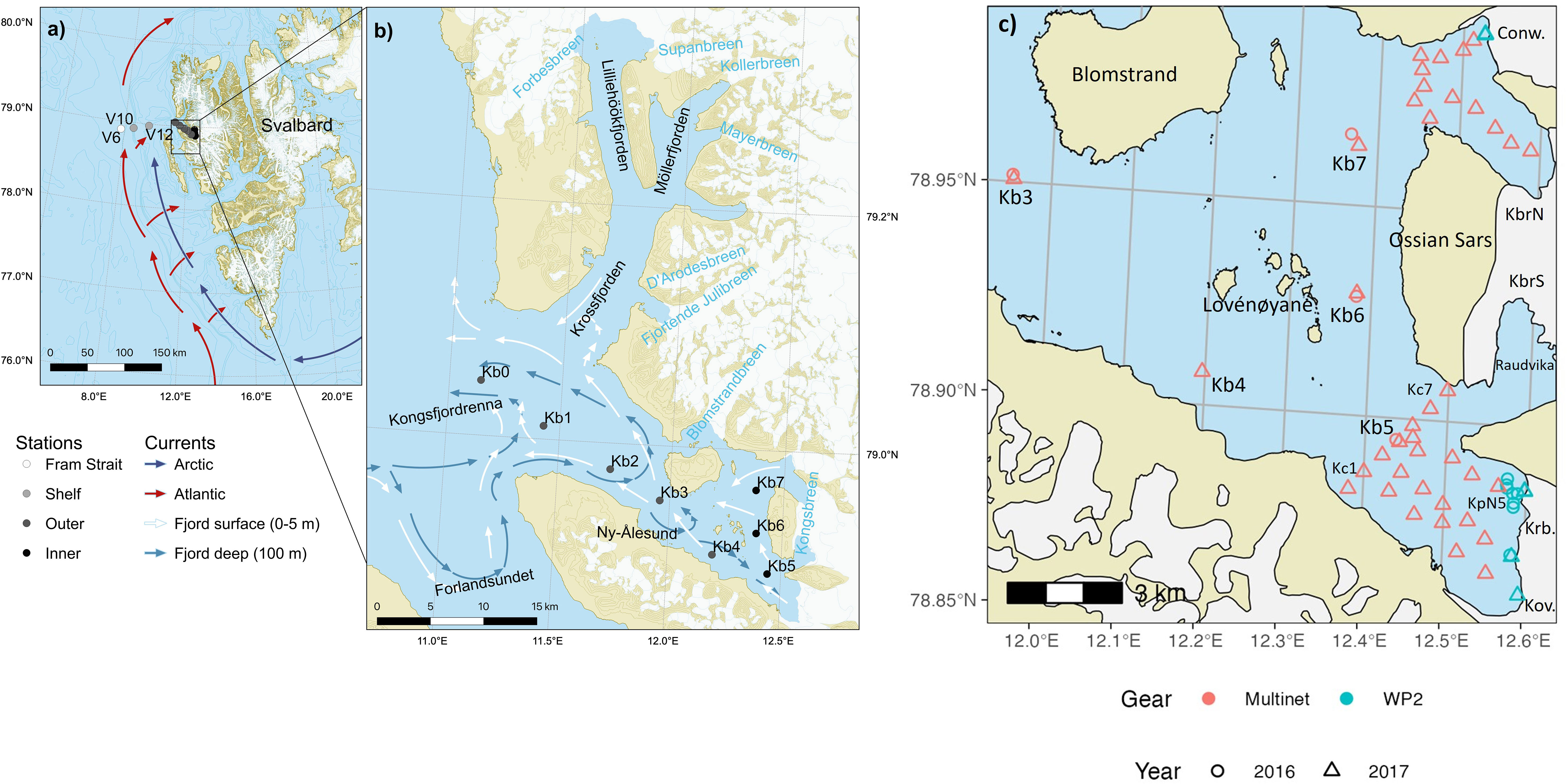
Figure 1 Kongsfjorden transect stations in (A) Shelf and shelf slope to Fram Strait (V6, V10, V12) with Atlantic and Arctic currents, (B) fjord stations with main circulation patterns indicated outside and inside the fjord (Modified from Hop et al., 2019), (C) Sampling stations with RV Lance and a helicopter in front of Kongsfjorden tidewater glaciers on 1-3 August 2016 and 25-28 July 2017. Red rings/triangles are Lance stations in 2016/2017 sampled with MultiNet, whereas cyan equivalents indicate helicopter sampling stations with WP-2 and WP-3 in the respective years. The sampling was more extensive in 2017 than in 2016, and the northern stations were only sampled in 2017. Glaciers are Conwaybreen (Conw.), Kongsbreen North and South (KbrN, KbrS), Kronebreen (Krb.) and Kongsvegen (Kov.). The location of main sampling stations (Kb4-Kb7) is referred to as inner fjord basin, whereas sampling near the glaciers are in the respective glacial bays (outer bay, mid bay and at the glacial front).

In the inner part of the fjord, the islands of Lovénøyane and the associated rising seabed, with a shallow sill (about 20 m deep) to the south and a deeper sill (50 m) to the north, form the inner basin of Kongsfjorden. There are four tidewater glaciers in the inner part of Kongsfjorden: Kongsvegen, Kronebreen, Kongsbreen, and Conwaybreen (Figure 1C). The inner fjord basin can be further divided into a northern glacial bay (max depth 125 m) and southern glacial bay (max depth 95 m), north and south of the Ossian Sars Mountain (Figure 1C). In the southern glacial bay, Kronebreen and Kongsvegen drain through a shared terminus which reaches around 50-60 m depth (Supplementary Figure S1). Kronebreen currently occupies about 70% of the glacier width at the terminus (Sund et al., 2011), and together these glaciers form the largest tidewater glacier terminus in Kongsfjorden. The main outflow from the glaciers was situated in front of Kronebreen at the time of the study. The part of Kongsbreen located south of the Ossian Sars Mountain (Kongsbreen South) is more influenced by the runoff from the Kronebreen-Kongsvegen system, which involves erosion of red sandstone into the glacial bay named Raudvika (red bay). Kongsbreen south and Raudvika were not included in our survey, but have been previously studied (Urbanski et al., 2017). The deepest parts of the bays surveyed in our study are located in the northern glacial bay, in front of Kongsbreen North, which sits partly on land. Conwaybreen rests largely (<70%) on bedrock above the water line. The northern glacial bay receives less run-off with sediments because Conwaybreen and Kongsbreen North erode hard rocks of marble, gneiss and granite (Dallmann, 2015).

The water temperature in the inner fjord basin is typically lower, or more Arctic, than further down fjord and offshore (Santos-García et al., 2023). It is suggested that such cold and saline waters are remnants of winter-cooled waters resulting from heat loss to the atmosphere and contact with glacial fronts (Torsvik et al., 2019). However, in summer, the mixing of meltwater from the glaciers with ambient seawater results in lower salinity (Torsvik et al., 2019). The water column in inner Kongsfjorden has warmed by 0.13 °C y^-1 at 35 m and 0.06 °C y^-1 at 85 m depth from 2010 to 2020, while salinity has increased by 0.3 (De Rovere et al., 2022). Depth-averaged temperatures have increased by 0.21°C y^-1 in the warmest months of the year, whereas they appear relatively stable in the coldest months (De Rovere et al., 2022).

Sampling by vessels and helicopter

The along-fjord transect in Kongsfjorden was taken with RV Lance both years, 25-28 July 2016 and 30 July-2 August 2017, from the inner fjord basin out to station V6 in Fram Strait at 1000 m depth (Hop et al., 2019; Figures 1A, B). The inner fjord with glacial bays was subject to more intensive sampling both years, because of the focus of the study on investigating the small-scale patterns and the potential effect of glacial run off on zooplankton survival.

Samples in front of tidewater glaciers were collected by helicopter and RV Lance in the glacial bays on 1-3 August 2016 and 26-31 July 2017 (Figure 1B). In 2016, four stations were sampled from RV Lance and eight stations were sampled by a helicopter in front of Kronebreen. The sampling was conducted around the North plume of Kronebreen. In 2017, the sampling campaign in the glacial bays was more extensive and included the bays in front of several glaciers around the inner basin. Sampling stations were clustered based on their similar hydrography and distance to glacier fronts in the southern and northern part of the glacial bays: Kronebreen-Kongsvegen (South) and Conwaybreen-Kongsbreen (North). The inner part of Kongsfjorden was surveyed with the research vessel for hydrography in 2017 from the inner transect station Kb5, with one transect across the outer glacial bay and one from Kb5 towards the glacial front of Kronebreen. Sampling closest to the glacial fronts was performed by helicopter also in 2017. In addition, a small surface net was pulled across the brown glacial plume in front of Kronebreen with a small vessel (AKVA Polarcirkel RBB) at a safe distance from a stable section of the glacial front. The hydrography was also surveyed outside Conwaybreen and Kronebreen North, as presented in Halbach et al. (2019).

Biogeochemical environmental variables such as nutrients, chlorophyll a (Chl a), phytoplankton and suspended matter were sampled both from RV Lance and by helicopter in close proximity to the glacier fronts. On board the ship, water samples were collected with 8L Niskin bottles mounted on a rosette sampler equipped with a CTD (conductivity-temperature-depth, Sea-Bird Electronics SBE911, Bellevue, WA, USA), photosynthetically active radiation (400-700 nm, PAR: Spherical underwater Quantum Sensor Li-193, LI-COR Biosciences) and fluorescence (WETStar, Sea-Bird Electronics) sensors.

From helicopter, sampling was done by means of a CTD rosette at 33-m distance to the Kronebreen front and 93-m distance to the Conwaybreen front. The Hydro-Bios Multi Water Sampler SlimLine 6 rosette equipped with an integrated CTD and 6×3.5 L Niskin bottles was attached 5 m above a 500 kg counterweight (cement drum), which was connected to a wire of 100 m length. Sampling was conducted by lowering the counterweight to the bottom, causing notable slack on the wire, and then pulling up slowly (1 m s⁻¹) with the ascending helicopter which was hovering well above the glacier. Thus, water samples were taken from the entire water column from 5 m above the bottom.

Zooplankton

Zooplankton sampling from RV Lance was done with a Multiple Plankton Sampler (MultiNet type Midi, Hydro-Bios Kiel), consisting of five nets with 0.25 m² opening and 200 µm mesh size, hauled at a speed of about 0.5 m s^-1 and closed in sequence. Depth strata sampled were bottom-200 m, 200-100 m, 100-50 m, 50-20 m, 20-0 m. For the shallow stations, the depth intervals were reduced (bottom-50 m, 50-20 m, 20-0 m). Zooplankton sampling from Polarcirkel was done in 2017 with a surface net (0.4 × 0.7 m opening, with 200 μm mesh) towed slowly at about 1 m s^-1 for estimated (GPS) distances of 244-1317 m (mean 617 m) in five tows.

For zooplankton sampling by helicopter, the CTD rosette was replaced by plankton nets: WP-2 (0.25 m² opening, 200 μm mesh) or WP-3 (1 m² opening, 1000 μm mesh). These were operated similarly, at same locations, sampling the entire water column from 5 m above the bottom (towing speed ca. 1 m s^-1), and samples were retrieved by a ground team.

The plankton nets used are known to sample mesozooplankton representatively, but tend to undersample both microzooplankton and macrozooplankton (Hop et al., 2019). The nets will collect some macrozooplankton, such as Themisto spp. and Thysanoessa spp., but predominately the smaller size classes. Logistically, in the glacial bays with icebergs and by sampling from helicopter, it was impossible to use larger nets, such as MIK and Tucker trawl, which would have sampled macrozooplankton and fish larvae-juveniles more efficiently (Hop et al., 2019).

Samples for taxonomical analyses were preserved with a hexamethylenetetramine-buffered formalin solution at a final concentration of 4% immediately after collection. For determining non-consumptive dead vs. live zooplankton in and around the glacial plume, samples from 2016 were subjected to neutral red staining. The stock solution was made according to Elliott and Tang (2009) and applied to zooplankton samples immediately after collections. After staining for 15 min, the sample was rinsed on 200 μm mesh and preserved with formalin at a final concentration of 4%. Subsequent analyses involved counts of stained (live) vs. not-stained (dead) organisms.

For taxonomic determination, organisms were identified and counted under a stereomicroscope equipped with an ocular micrometre, according to standard procedures, including morphology and prosome length for Calanus spp. (Postel et al., 2000; Kwasniewski et al., 2003). Other zooplankters were identified to the lowest possible taxonomic level based on available literature and web descriptions. The zooplankton were separated into groups for presentation in figures: small copepods (< 2.5 mm total length as adults), large copepods as Calanus species (C. finmarchicus, C. glacialis, C. hyperboreus), other large copepods (e.g., Metridia longa and Paraeuchaeta spp.), meroplankton (e.g., Bivalvia, Echinodermata, and Polychaeta), other zooplankton (e.g., Fritillaria borealis, Limacina helicina, Parasagitta elegans). The dry mass conversion factors from Hop et al. (2019) with subsequent updates (Assmy et al., 2023) were applied for calculating zooplankton biomass.

The abundances (ind. m^-3) or biomasses (mg dry mass (DM) m^-3) for each species or a group of species were summed up by stage, size group and/or species and averaged over depth strata for each station using the following equation:

where $a_i$ is the abundance or biomass of species a at depth stratum i, $d_i$ is the sampled distance for depth stratum i in meters, D is the total depth of net haul, and n is the number of depth strata at a station. In order to compare all stations of the fjord and shelf transect to V6, only data from the upper 200 m were included or bottom if shallower (inner part). Abundances were expressed as ind. m^-3 to be able to compare with earlier studies (e.g., Kwasniewski et al., 2003; Walkusz et al., 2009; Kwasniewski et al., 2013; Hop et al., 2019). Since samples from the inner part of the fjord were taken shallower (40-50 m) than mid-fjord samples (upper 200 m), we also presented the number of zooplankton as ind. m^-2, which expresses the total number of organisms at a site (Circle plots in Supplementary Figures S1–S3; Supplementary Tables S1, S2).

Benthic amphipods

Benthic amphipods were caught in baited traps, in strings of five traps each deployed overnight from Polarcirkel at different locations in the glacial bay outside Kronebreen in 2017. The baited traps consisted of plastic pipe (20 cm long, 10 cm in diameter) with a funnel attached to one end and a removable net (mesh size: 1 mm) on the other. Bait was raw chicken meat packed in fine-mesh bags to prevent the amphipods from getting access to it (Nygård et al., 2009). The collected scavenging species were identified under a stereomicroscope.

Stable isotope analysis

Samples for stable isotopes were obtained from MIK and WP-3 net hauls from the entire water column performed at the sampling stations (Table S7). Some of the fish were caught in those nets, whereas larger specimens of Atlantic cod (Gadus morhua) and haddock (Melanogrammus aeglefinus) were caught by jigging from the research vessel. Samples for stable isotopes δ¹⁵N and δ¹³C were prepared according to the method described by Søreide et al. (2006a) and Søreide et al. (2006b), with removal of lipids and carbonates from samples in order to reduce variability. They were analysed at the Institute for Energy Technology, Kjeller, after the same procedure as described in Søreide et al. (2006b).

Stable isotope data provide quantitative information on the resources that a community uses (bionomic) and its bioclimatic habitat (scenopoetic). This information can be used to define the community’s ecological niche (Newsome et al., 2007). A difference in ecological niche would indicate a difference in primary carbon sources and the background bioclimatic conditions (Jackson et al., 2011). An ecological niche can be represented as an n-dimensional hyperspace that can be partitioned into scenopoetic axes, representing environmental components of niche space, and bionomic axes, which refer to the trophic components of niche space (Hutchinson, 1978). Location on these axes can be quantified using stable isotopic ratios (Jackson et al., 2011) and formalized in the concept of the ‘isotopic niche’ (Newsome et al., 2007). It is important to note that ‘isotopic niche’ does not explicitly define an ‘ecological niche’ as it does not typically provide species or taxon information on resource use. Instead, within the broad domain of ‘ecological niche’, it can provide a useful summary of ecological characteristics such as primary carbon sources of each area (glacial bay, inner and outer fjord).

Various metrics have been proposed to analyse the spread of data points within the n-dimensional hyperspace defined by the bionomic and scenopoetic axes to quantify the ‘isotopic niche’ (Jackson et al., 2011). To date, the most useful has been to calculate the convex hull area (TA) encompassing the data points (Supplementary Figure S5), providing an indication of the niche width of each community in question (Layman et al., 2007; Jackson et al., 2011). A significant shortcoming of this approach, relevant to our study is high sensitivity to sample size and composition (Jackson et al., 2011). Instead of convex hulls, we have used an alternative approach based on standard ellipses (Batschelet, 1981), reformulated in a Bayesian framework (Jackson et al., 2011). This allows robust comparison between data sets (Supplementary Table S9 ) comprising different sample sizes accounting for uncertainty. The computational code to calculate the metrics is available in the free-to-download package Stable Isotope Analysis for R (SIBER).

Data analysis

Positions of glacier fronts were estimated by vectorising the fronts from a Sentinel-2 satellite photograph taken on 31 July 2017 (see Halbach et al., 2019). Euclidian distance of each station to the closest front was then calculated using a UTM projection (epsg:32633) and the st_distance function from the sf package (Pebesma, 2018) for R (R Core Team, 2022).

The relation of total zooplankton biomass and abundance to the distance from the closest glacier front was examined using log-linear [lm(log(total) ~ log(dist)] and general additive [gam(log(total) ~ s(log(dist))] models. We performed a principal component analysis (PCA) on a square root transformed proportion species composition matrix [i.e., “Hellinger transformation” in Legendre and Gallagher (2001)]. The analysis was performed using the rda function, and the transformation using the decostand function from the vegan package (Oksanen et al., 2022) for R.

Results

Oceanographic conditions for Kongsfjorden and the shelf were characteristic for the summer situation in late July, with rather similar conditions in 2016 and 2017 (Figures 2A–D). Relatively warm (6-8°C) surface waters with reduced salinity (<30), increased in vertical extent towards the inner fjord basin. Transformed Atlantic Water constituted most of the water mass in the fjord. In both years, TAW with temperatures 2.5-3.0°C extended to the bottom.

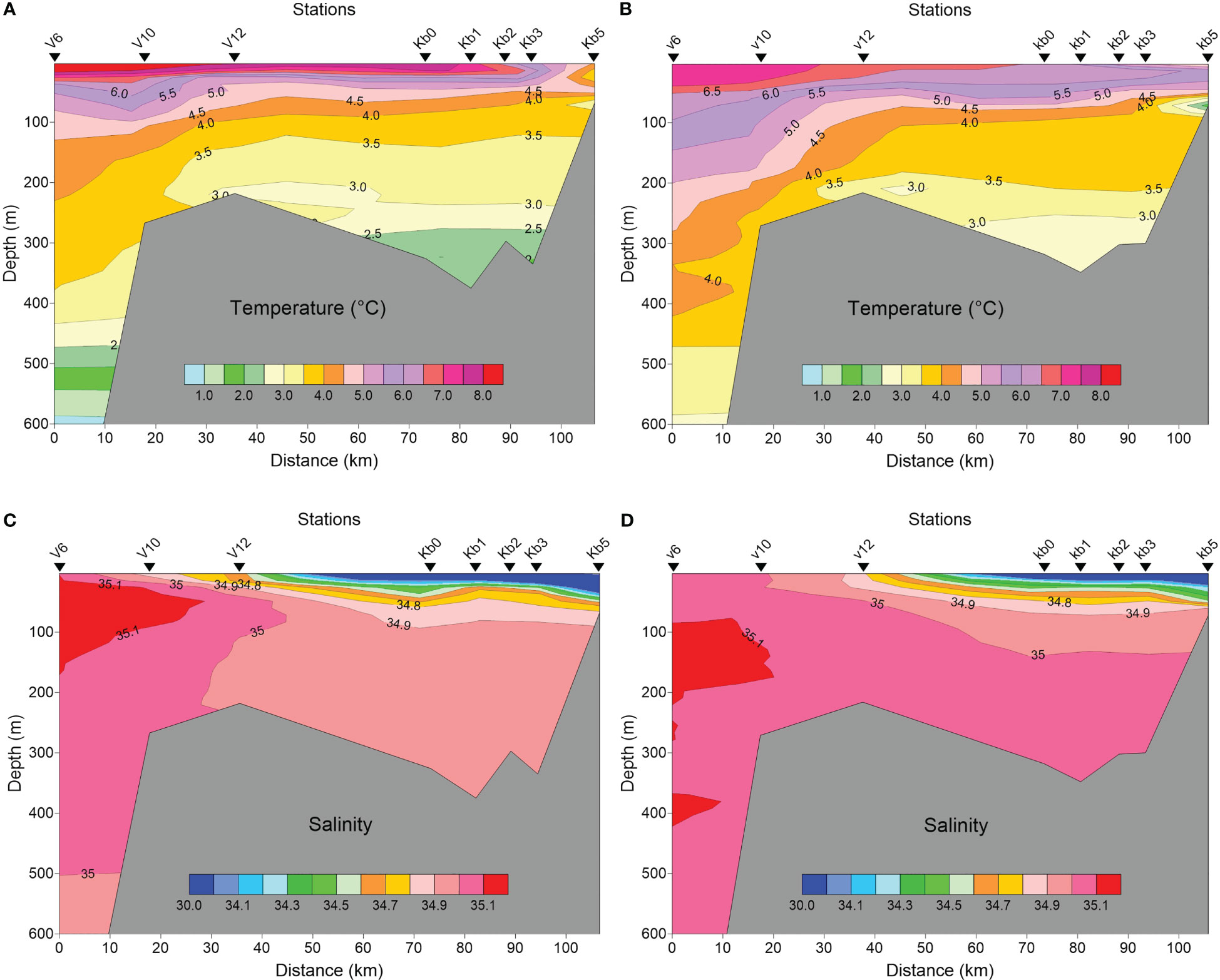
Figure 2 Temperature (A, B) and salinity (C, D) profiles along Kongsfjorden from V6 in Fram Strait to station Kb5 in the inner basin in late July 2016 (A, C), and late July-early August 2017 (B, D).

The water column in the inner part of Kongsfjorden, based on measurements from 2017, was stratified, even behind the inner sill of 50 m depth (Figures 3A–D). The temperature varied from 5.5°C in surface waters to 1.5°C near the bottom at 70 m depth. The glacial effect, including both glacial river discharge and direct ice melting, caused some freshening of the surface layers to <30, but no salinity values below 26 (Figure 4). The glacial effect was not very strong even at the innermost station sampled (KpN5), which was about 1 km from the main glacial water outlet at Kronebreen. The fresher surface water only comprised the upper 5 m of the water column and became further reduced outside the sill. Atlantic water and TAW prevailed in the deeper parts (>50 m depth) in the fjord, and extended to the inner fjord basin and glacial bays (Figure 4).

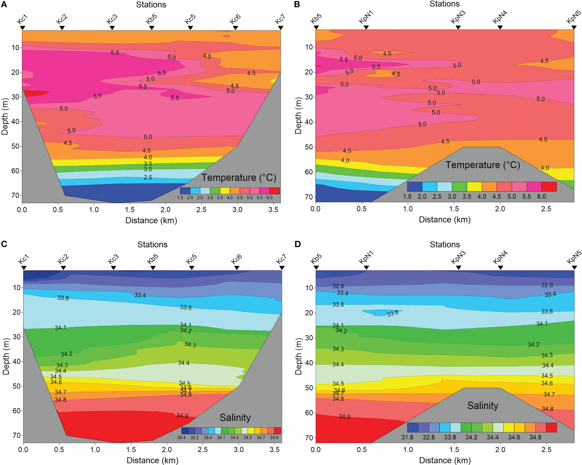
Figure 3 Temperature (A, B) and salinity (C, D) in the glacial bay of Kongsfjorden in late July 2017  across the southern glacier bay (Kc1 via Kb5 to Kc7) (A, C), and from station Kb5 (Figure 1) to the glacial front of Kongsvegen/Kronebreen (station KpN5) (B, D).

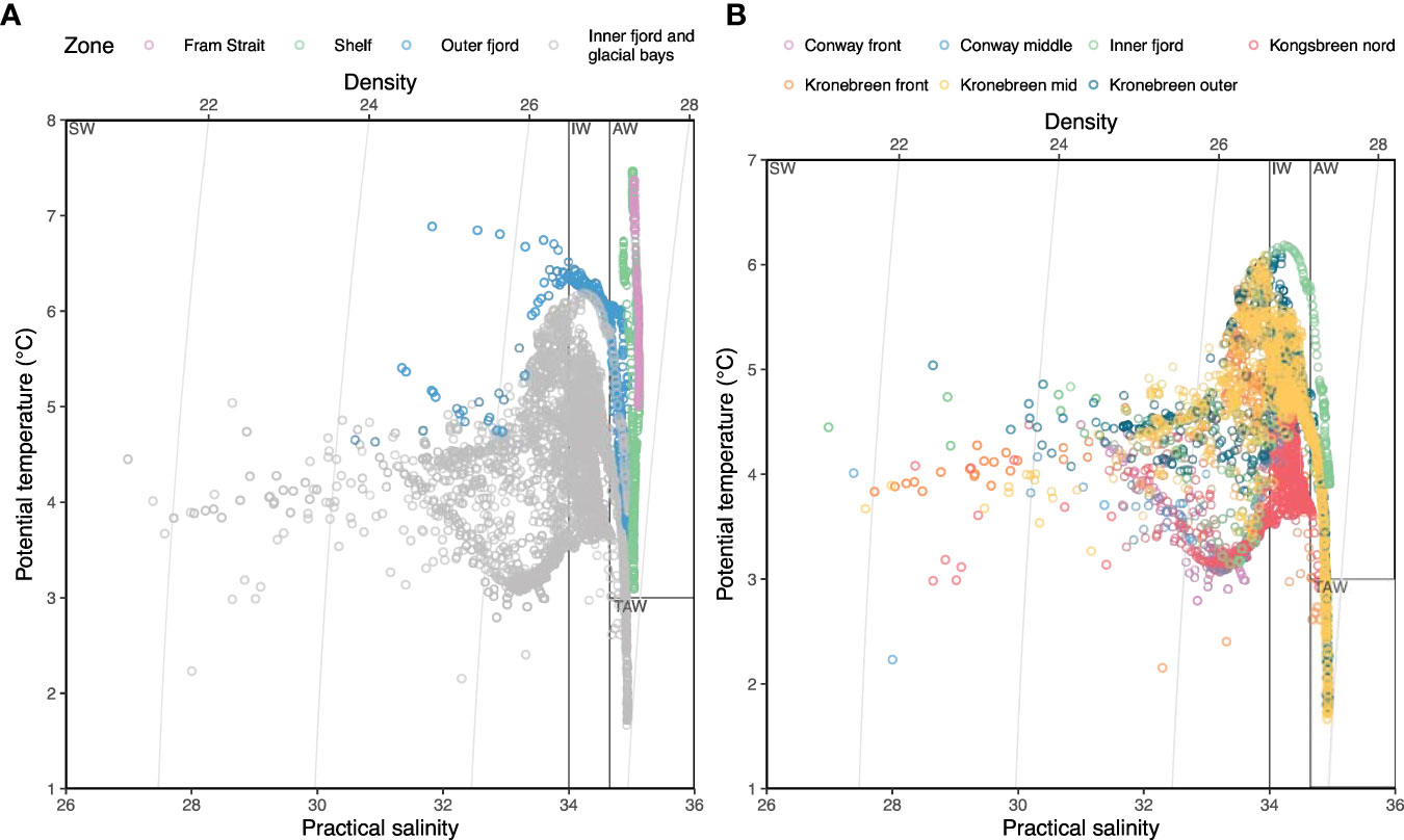
Figure 4 Temperature-salinity plots showing water masses in the upper 200 m in the entire study area (A) and only the inner fjord and glacial bays (B) in 2017. Ten observations with salinity < 5 from Conway-front and Kronebreen-front have been removed to make the plots readable. Water mass classifications follow those of Cottier et al. (2005): SW, surface water; IW, intermediate water; AW, Atlantic water; TAW, transformed Atlantic water.

Zooplankton distribution (in terms of abundance and biomass) at stations along the main fjord transect) is described below, and zooplankton distribution at stations in the inner fjord basin and glacial bays then follows.

The three Calanus species showed variable abundance in the upper 200 m along the transect, with generally higher abundance and biomass in early August 2016 than in late July 2017 (Tables 1A, 1B; Supplementary Figure S1A. One exception was the high abundance (1330 ind. m^-3) of Calanus finmarchicus in the inner fjord station Kb5 in 2017. The biomass of C. finmarchicus was generally high (> 150 ind. m^-3) in 2016 and 2017 both in the inner fjord and at the outer shelf break (V6), where Atlantic water masses prevailed. The Arctic C. glacialis showed variable lower abundance, but higher contribution to biomass within Kongsfjorden, with highest abundance values in the inner fjord basin (140 ind. m^-3) in August 2016, and lower abundance (50-60 ind. m^-3) in the inner fjord in 2017. Calanus hyperboreus was present but contributed little to abundance (generally <10 ind. m^-3) or biomass (Tables 1A, 1B).

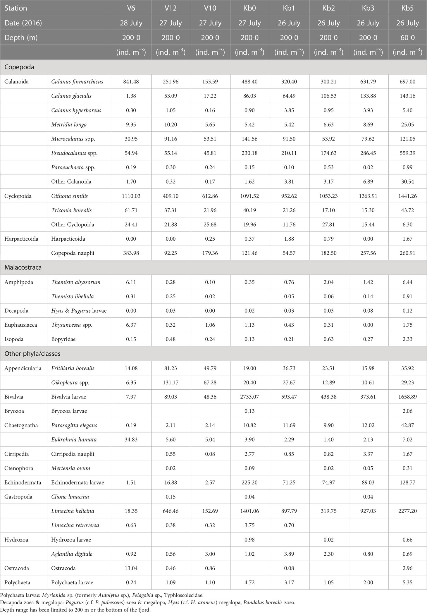
Table 1a Zooplankton abundance (ind. m^-3) at stations in Kongsfjorden, from inner fjord basin to outer fjord in July 2016.

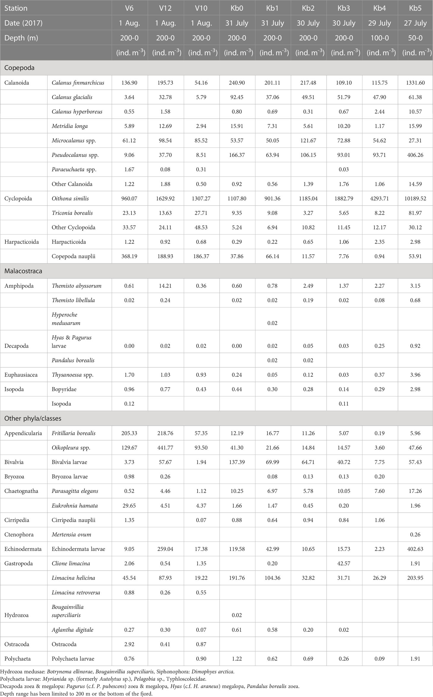
Table 1b Zooplankton abundance (ind. m^-3) at stations in Kongsfjorden, from inner fjord basin to outer fjord in July-August 2017.

The distribution of zooplankton biomass in relation to the distance from the glacier did not show any well-defined statistical trend; it was relatively even (lm log(dist) p = 0.17, gam s(log(dist)) p = 0.33). Despite this, the community differed with the distance showing spatial and annual variation (Figure 5). MultiNet covered a wider range in the PCA space (i.e. contained more species) than WP-2, mainly because there were more MultiNet casts in the dataset (Figure 5B). The results show that in 2017 there were more C. finmarchicus than in 2016, but this was mostly because high biomass of C. finmarchicus was found in samples from Conway- and Kronebreen stations (Table 2A; Supplementary Table S4B), which were collected only in 2017 (Figures 5C, D). As a result, C. finmarchicus showed generally a negative correlation with distance from closest glacier front (Figure 5E). Also C. glacialis demonstrated negative correlation with distance from the closest glacier front. The mean biomass of C. glacialis appeared uniform within Kongsfjorden and decreased on the continental shelf. Calanus hyperboreus showed to some degree negative biomass trends with distance from the closest glacier front. On the contrary, the chaetognath Eukrohnia hamata demonstrated the opposite correlation being more abundant on the shelf than in the fjord and glacial bays, although it also had a high biomass in some Kronebreen front stations (Figures 5D, E).

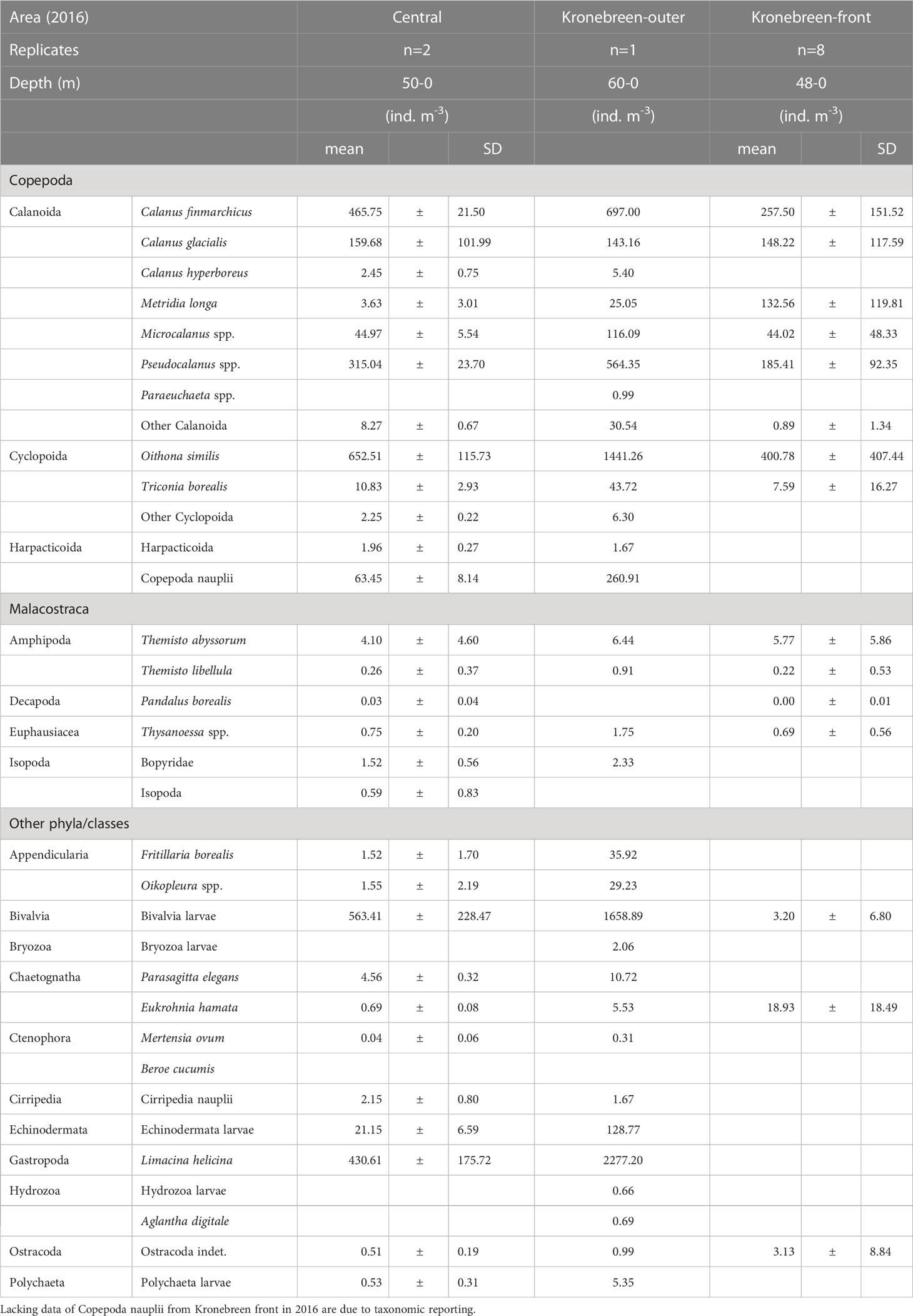
Table 2A Zooplankton abundance (ind. m^-3) in the inner central basin and glacial bay near Kronebreen, early August 2016.

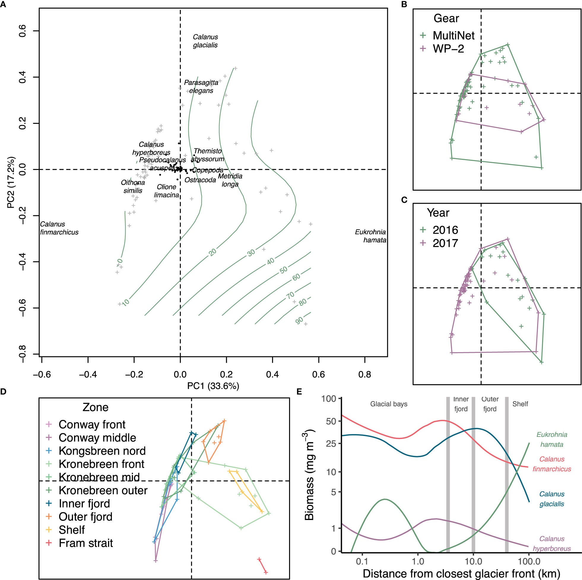
Figure 5 Principal component analysis of Hellinger transformed zooplankton biomass in Kongsfjorden. (A) Main species contributing to variation in biomass. Grey crosses indicate stations and green contour lines distance from the closest glacier front. Envelopes for (B) gear, (C) year and (D) zone in the fjord. Colours refer to the variable. (E) LOESS averages of biomass of most contributing species in (A) related to distance from the closest glacier front. Grey lines give approximate locations in Kongsfjorden. Both axes are logarithmic.

Small zooplankton was dominated by Oithona similis at all stations, with abundance values in the 400-1500 ind. m^-3 range in 2016 (Table 1A; Supplementary Figure S1B). The abundance of this species was generally higher in 2017, increasing towards the inner fjord basin (10,000 ind. m^-3 at station Kb5; Table 2A). Pseudocalanus spp. were the second-most abundant small copepods, both years, with highest density (400-550 ind. m^-3) at the inner basin station Kb5, and <300 ind. m^-3 in the middle and outer reaches of the fjord, with highest abundance in 2016. Copepoda nauplii showed variable abundance, and could be high both at the outer stations (200-400 ind. m^-3) and in the middle to inner part of the fjord (200-260 ind. m^-3). Microcalanus spp. were less abundant (30-120 ind. m^-3) with no clear pattern. The biomass contribution generally reflected the abundance pattern, although with larger contributions of Pseudocalanus spp., particularly at Kb5 in the inner fjord basin in 2016.

Other large copepods were mainly represented by Metridia longa and Paraeuchaeta spp., but also included less abundant species of the genera Aetideopsis and Scaphocalanus present at stations outside the main fjord basin. This group as a whole, however, was most abundant at Kb5 in the inner basin during both years, with 16-25 ind. m^-3 for M. longa and <1 ind. m^-3 for Paraeuchaeta spp. (Supplementary Figure S1C). Other large copepods had considerable biomass in the outer shelf region out to V6, but the highest was recorded for station Kb1 and Kb0 in the outer deep part of Kongsfjorden, and the main contributor to biomass was Metridia longa. Biomass of large copepods was generally higher in 2016 than in 2017.

Meroplankton included mainly larvae of Bivalvia and Echinodermata (Tables 1A, B; Supplementary Figure S1D). Bivalvia veligers and juveniles reached high abundance values (>1600 ind. m^-3) in the glacial bay in 2016 and occasionally also further out in the fjord (2700 ind. m^-3 at station Kb0). A similar pattern can be seen for 2017, although the abundance was much lower (Supplementary Figure S1D). Echinodermata larvae were less abundant with high values in the glacial bay (130-400 ind. m^-3) both years, and also highest abundance (260 ind. m^-3) outside Kongsfjorden on the shelf (station. V12) in 2017.

Other zooplankton were mainly represented by the pteropod Limacina helicina, the appendicularian Oikopleura spp. and the chaetognath Parasagitta elegans (Tables 1A, B; Supplementary Figure S1E). Particularly L. helicina was abundant as veligers in the inner fjord basin (2300 ind. m^-3 at Kb5) and also in the outer reaches of Kongsfjorden and Kongsfjordrenna (1400 ind. m^-3) in 2016. In 2017, the abundance of L. helicina was generally low (<90 ind. m^-3), except for at the inner fjord basin and outer fjord, also for veligers (200 ind. m^-3). Oikopleura spp. were only occasionally abundant at single stations (e.g., 440 ind. m^-3 at V12 in 2017; Table 2A). Parasagitta elegans was generally not abundant, but with some elevated abundance (17-43 ind. m^-3) at the inner station in both years, and lower abundance (10 ind. m^-3) in the outer part of the fjord in 2017. Because of its size, however, its contribution to biomass at the inner basin (Kb5) was relatively large. Less abundant species included Clione limacina, Themisto spp., Thysanoessa spp., and Meganyctiphanes norvegica, but because of their large size, their contribution to biomass could be considerable (Supplementary Figure S1E).

The inner fjord basin and glacial bays near the tidewater glaciers were subject to the most intensive sampling both years. The abundance of both Calanus finmarchicus and C. glacialis was high both near the glacial front and further out into the inner fjord basin (Table 2B; Supplementary Figure S2A). However, C. hyperboreus was mainly present at low abundance away from the glacial front. Of other large copepods, the abundance of small copepods in 2016 was generally high, particularly of Oithona similis and Pseudocalanus spp. (Table 2B; Supplementary Figure S2B). The abundance and biomass were variable, but with similarly high values close to the glacial front and further out into the inner basin. Copepoda nauplii also showed variable abundance, with highest densities in the outer part of the glacial bays. Metridia longa was abundant at the glacial front as well as further out in the glacial bay, but lower in the central part of the inner fjord basin (Supplementary Figure S2C). Meroplankton, represented by Bivalvia and Echinodermata, was abundant in the glacial bay and further out in the fjord basin, but nearly absent at the glacial front (Supplementary Figure S2D). Bivalvia constituted most of the biomass. Limacina helicina showed a similar distribution pattern, with highest abundance away from the glaciers (Supplementary Figure S2E). Other taxa, such as amphipods (e.g., Themisto spp.), were more abundant close to the glacial front.

Table 2B Zooplankton abundance (ind. m^-3) in the inner central basin and glacial bays, late July 2017.

In 2017, the three Calanus species. were homogenously distributed within the glacial bays, with C. finmarchicus and C. glacialis as the most abundant species. Calanus glacialis was more abundant in the glacial front areas than in the outer and central locations, although this was less apparent for biomass (Table 2A; Supplementary Figure S3A). As in 2016, small copepods were omnipresent in 2017, but with no clear pattern regarding the location in glacial bays or distances from the glacial front (Table 2A; Supplementary Figure S3B). As before, the biomass followed the abundance values of these small copepods, with larger contribution of Pseudocalanus spp. Other large copepods, such as Metridia longa, were also more abundant and with higher biomass in the glacial front areas of Kronebreen than further out in the glacial bays and the central part of the inner fjord basin (Supplementary Figure S3C). However, Paraeuchaeta spp. were only found in the middle glacial bay and were not present at the fronts. The meroplankton was variable, with high abundance of Bivalvia at the Conwaybreen front and high abundance of Echinodermata at the Kronebreen front (Supplementary Figure S3D). The biomasses showed the same split for Bivalvia and Echinodermata, but within each location the taxa were more evenly distributed from bay to the glacial front. Other meroplankton, such as polychaetes and gastropod veligers, were occasionally abundant in the glacial bays, with polychaetes contributing with the largest biomass (Supplementary Figure S3D). Limacina helicina and Parasagitta elegans were rather evenly distributed within the glacial bays, with L. helicina as the most abundant species contributing largely to the biomass at the glacial front of Kronebreen (Supplementary Figure S3E). Because of their larger sizes, Parasagitta elegans and other taxa contributed most to the biomasses at the glacial fronts (Supplementary Figure S3E).

In the close vicinity of the glacial front, zooplankton abundance was variable between years (Tables 2A, B). In 2016, the abundance of zooplankton was generally lower close to the glacial front than further out in the glacial bay and in the central basin. The opposite was true for 2017, when there were higher abundances inside the plume close to the glacial front, particularly for Calanus finmarchicus, C. glacialis, Metridia longa and Pseudocalanus spp. The abundance was higher outside of Kronebreen/Kongsvegen and lower outside Conwaybreen/Kongsbreen in 2017. Close to the surface, based on the surface net tow performed close to the glacial front of Kongsbreen, the zooplankton abundance was, nonetheless, not higher than the average for the water column within the plume (Table 2A). It also needs to be remembered that the mean abundance values (ind. m^-3) for the glacial bay stations are based on sampling within shallower depths (40-60 m) than for the mid-fjord stations (upper 200 m). Abundances expressed as ind. m^-2 (Circle plots in Supplementary Figures S1–S3; Supplementary Tables S1, S2) show that some dilution effects are apparent for the deeper samples. Biomass values (mg m^-3) tend upgrade large organisms such as Calanus spp., chaetognaths and other large zooplankton, and downplay smaller forms, such as cyclopoid and harpacticoid copepods, and meroplankton (Supplementary Tables S3, S4).

Neutral Red staining, applied to samples in 2016, showed that most zooplankton were alive both inside and outside the plume (Figure 6). Only a small percentage (< 5%) of dead zooplankton was recorded inside the plume, and none outside. WP-2 catches consisted mainly of Calanus copepods. Calanus glacialis comprised the bulk of biomass both in WP-2 and WP-3 nets, seconded by C. finmarchicus and M. longa. Of other zooplankton, chaetognaths and Themisto spp. contributed with largest biomasses in both nets.

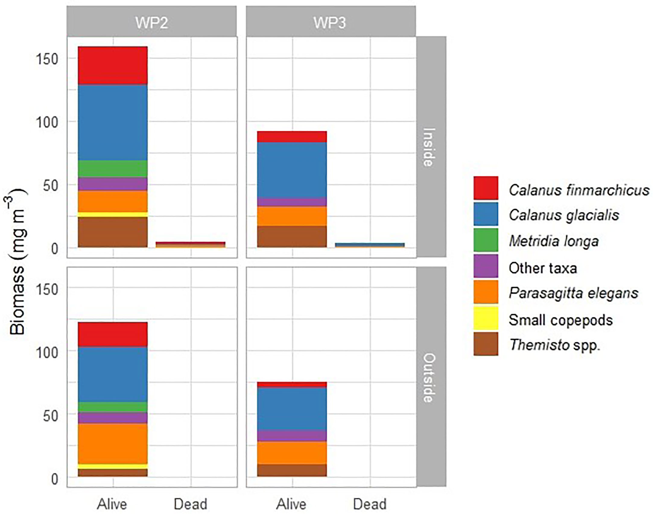
Figure 6 Biomass of alive and dead zooplankton sampled inside and outside the glacial plume from helicopter in July 2016 with WP-2 and WP-3 net.

The composition of dead zooplankton was dominated by Calanus copepods and chaetognaths, whereas amphipods Themisto spp. and Onisimus litoralis, krill Thysanoessa spp., and shrimp Pandalus borealis were less affected (Figure 7). Of copepods, Calanus finmarchicus was more abundant than C. glacialis in the dead zooplankton fraction. Dead zooplankton concentrations were up to 6 mg DM m^-3 in front of Kronebreen, but typically outside the centre of the plume, which had the lowest salinity (Figures 8A, B). The salinity in the upper meter was brackish, but never<30 in the upper meter (Figure 8B). In surface samples taken with a bucket in 2017, the salinity varied between 22.0 and 30.3.

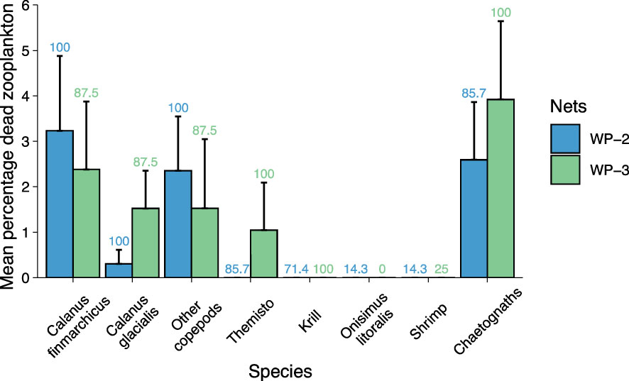
Figure 7 Composition of dead zooplankton as mean percentage (+SE). Numbers above bars are frequency of occurrence of a given group in all helicopter samples from early August 2016.

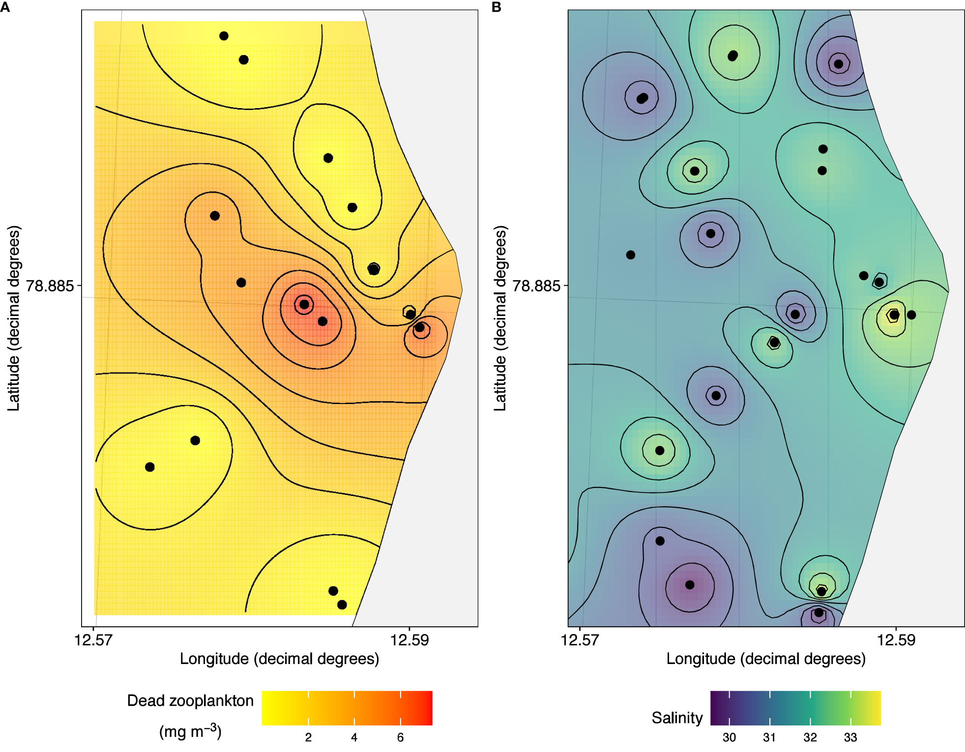
Figure 8 Interpolated distribution of (A) dead zooplankton (dry mass, mg m^-3), (B) salinity in the upper meter of the water column in front of Kronebreen, 1-3 August, 2016. The easternmost point marks the centre of the plume.

Three probable distinct isotopic niches were identified using our Bayesian inference approach. We classified these as the glacial bay, mid-fjord and shelf isotopic niche communities (Figure 9). The glacial bay community showed the widest isotopic niche suggesting a wider source of primary carbon sources to zooplankton compared to the other niches and a different scenopoetic environment. The composition of zooplankton and fish in our samples were also different (Supplementary Table S5).

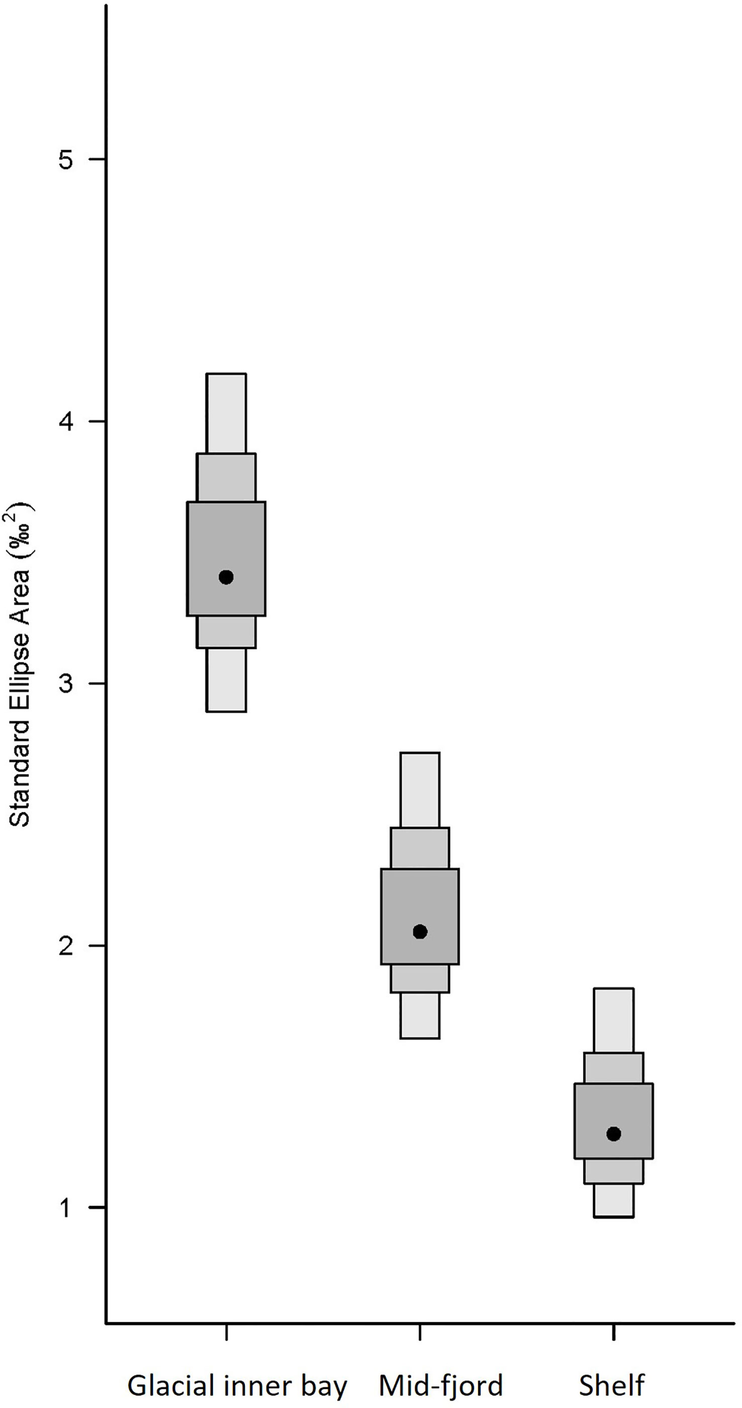
Figure 9 Isotopic niche width based on analyses with Bayesian inference. Shaded boxes represent the 25%, 75% and 95% confidence intervals (from dark to light grey) and black dots represent centre of mass of each community centroid. Isotope scatter plot of the raw data overlaid with ellipses the Bayesian Standard Eclipse Area for each community group (glacial bay, mid-fjord and shelf) is in Supplementary Figure S2.

Benthic scavengers, Onisimus caricus and Anonyx nugax, caught in baited traps were present and relatively abundant at and near the brown plume with daily catches of 10 animals per trap (Figure 10). However, the highest abundance was further out in the glacial bay, with up to 50 animals per trap per day, with 75% share of Anonyx spp. and 25% or less O. caricus.

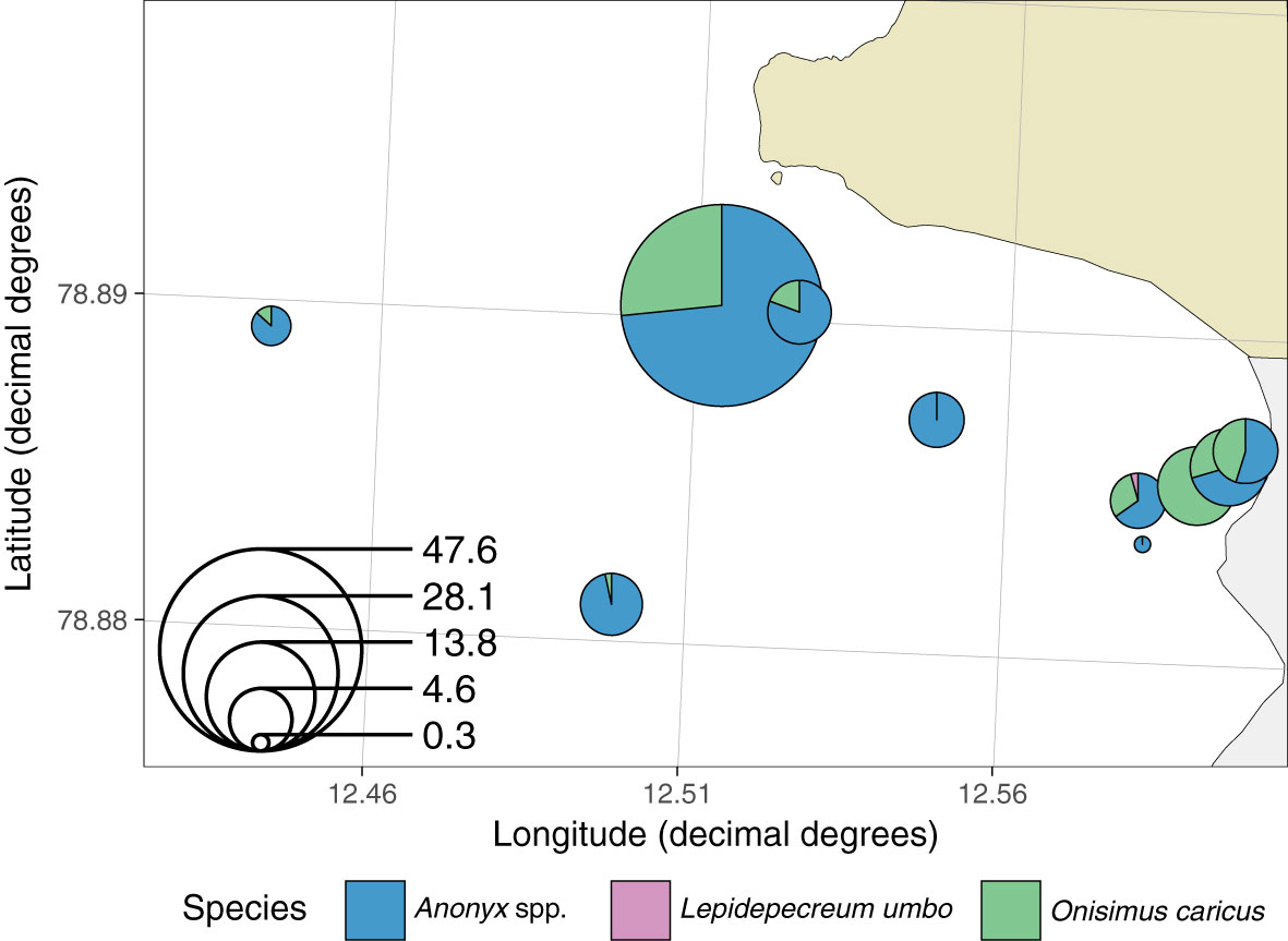
Figure 10 Amphipods caught in baited traps in the glacial bay in front of Kronebreen, 2017. Pie size indicates catch per unit of effort (CPUE as ind. per trap day), and the colours in pies indicate shares of different scavengers in the unit catch, their relative abundance.

Discussion

We found that zooplankton mortality in the “death trap”, indicated by Weslawski and Legezynska (1998), was not high as measured by neutral red staining of dead zooplankton. Thus, the studied glacial run offs did not appear to induce high zooplankton mortality, at least based on our snapshot-observations. Zooplankton is supposedly killed or stunned by osmotic shock, but our transect towards the glacier did not indicate very low salinity levels at the surface, certainly not at the brackish levels (salinity 9) used in experiments by Zajaczkowski and Legezynska (2001). The surface water salinity we observed in the glacial bay in front of Kronebreen was 30-33 in the upper 5 m, which is similar to seal-collected CTD data from the terminus of Kronebreen (Everett et al., 2018). Thus, the salinity near the surface in the inner glacial bay was not close to that causing zooplankton mortality in low-salinity experiments (Zajaczkowski and Legezynska, 2001), and the duration of exposure to fresher water deeper in the plume was likely short. The study by Everett et al. (2018) suggests continued mixing of glacial discharge water with ocean water between 40 and 0 m, which brings the water at the surface back to near-marine salinity conditions. The mixing during summer with dispersion of salinity is further elaborated by Torsvik et al. (2019). The prevailing down-fjord katabatic winds enhance this vertical mixing of the glacier discharge and fjord waters near the glacier front and contribute to the outflow of fresher surface water along the northern shore.

Seasonally, the mortality of zooplankton is much greater during the winter than in summer, when our study was conducted. Even if non-consumptive mortality in zooplankton is rarely reported, a few studies have detected high percentages of dead zooplankton in samples from the winter season. Daase et al. (2014) caught zooplankton in the southern Nansen Basin north of Svalbard in January 2012, of which 94% were dead. A wider study with seasonal sampling at several locations in Svalbard, found 11-35% dead copepods during winter, and 2-12% during spring and summer (Daase and Søreide, 2021). The spring/summer estimates are comparable to the 0-6% found in this study. Calanus spp. contributed most to this mortality, particularly during winter. Mortality was also observed in smaller copepods, such as Pseudocalanus spp., Microcalanus spp. and Oithona similis, whereas other zooplankton contributed little. Daase and Søreide (2021) did not sample close to glacier fronts and could not link mortality to osmotic shock. They rather suggested that insufficient energy stores to sustain activities throughout winter contributed mostly to the non-consumptive mortality.

Abundance and biomass of zooplankton generally increased in the inner fjord basin compared to most transect stations in middle and outer fjord. This particularly applied to Arctic species, such as Calanus glacialis and Limacina helicina, but also older life stages of Atlantic species, which showed high biomass in the basin and glacial bay. This is in line with previous work by Kwasniewski et al. (2003), who related the abundance and biomass to stage development of Calanus spp. and fjord circulation patterns. Some of the zooplankton species, such as C. finmarchicus and Limacina helicina, showed large variations between years, which may be reflected in their 2-year life cycles (Kwasniewski et al., 2003; Gannefors et al., 2005) or related to annual differences in water-mass advection to Kongsfjorden (Tverberg et al., 2019).

We suggest that advection is the dominant process for the observed pattern in zooplankton distribution. The sampling in 2016 and 2017 indicates similar spatial variations in zooplankton distribution, within the circulation pattern and upwelling of “deep” waters with high zooplankton abundance of older stages between the 20 m deep sill before the inner fjord basin and the 50 m deep sill before the glacial front. The largest zooplankton concentrations of C. finmarchicus in 2016 were recorded 1-3 km away from the glacial front, in the inner fjord basin (at Kb5), whereas in 2017 this species was more evenly distributed in the glacial bay. Calanus glacialis showed the opposite pattern in 2017 and was most concentrated close to the glacial front and in the bay near the glacier, but with lower concentrations in the inner fjord basin. The annual hydrographic conditions in Kongsfjorden seemed rather similar for 2016 and 2017, both on an increasing trend of temperature (0.13°C y^-1; Feldner et al., 2022). Thus, the years of sampling were not extremely warm or cold with resulting influence on the composition of Atlantic vs. Arctic zooplankton.

The younger zooplankton stages are mostly associated with surface waters and may have originated on the shelf outside the fjord. They are advected in surface and subsurface waters into the fjord and subsequently into the inner fjord basin as they develop (Basedow et al., 2004; Willis et al., 2006). Thus, a combination of ontogenetic growth and advection result in increased abundances of older stages (CIV-CV) and adult females in the inner basin. The oldest copepodid stages (CV) of C. glacialis were mostly deep in the inner basin whereas C. finmarchicus stages were more evenly distributed in the water column (Basedow et al., 2004). The advection of C. finmarchicus is higher than C. glacialis, which may be more locally produced (Basedow et al., 2004). By descending the zooplankton prevent being transported out of the inner basin by the outgoing surface currents. Also, descending, especially in late summer by older, wintering life stages, may be a way to avoid increasing water temperature (Kosobokova, 1999; Kwasniewski et al., 2003). The entrance to the inner basin is mainly along the southern shore, whereas the exit is along the northern side of the glacial bay where subglacial discharges release freshwater and sediments in front of the tidewater glaciers (Halbach et al., 2019) and this flow continues further out into the fjord basin and the transitional zone of the main fjord (Hop et al., 2002).

The abundance and biomass of the zooplankton in the glacial bays may also be a consequence of the glacial run-off, which contributes nutrients to the inner glacial bays (Halbach et al., 2019). The seasonal run-off from glaciers, with associated nutrients, are expected to fuel the summer blooms of mixed communities, involving diatoms, the prymnesiophyte Phaeocystis pouchetii and particularly smaller flagellates (Piwosz et al., 2009; Calleja et al., 2017; Halbach et al., 2019; Assmy et al., 2023). Some studies have documented massive blooms near the glacier front, in the inner basin, prior to the main run-off season in spring (Calleja et al., 2017), whereas others have documented later blooms in the middle or outer fjord (Hegseth and Tverberg, 2013). Where and when blooms are occurring are important for feeding and development of zooplankton populations (Daase et al., 2013).

Our stable isotope analysis revealed that the glacial bay houses a separate and wider isotopic niche than communities outside the sill to the inner fjord basin. As the isotopic niche is defined by δ¹⁵N and δ¹³C, this does imply different primary carbon and nitrogen sources for this zooplankton community (Santos-García et al., 2023). It is unknown to us at present if the community of zooplankton and fish represents a different trophic niche as isotopic niche is not necessarily correlated to the trophic niche (Jackson et al., 2011). More extensive sampling for stable isotopes than what was possible within the time frame of our study could help better interpreting such results. Thus, further work on the trophic structure of the glacial bays vs. the main parts of the fjord is required.

The physics of subglacial plumes with impact on fjord circulation is well established (e.g. Everett et al., 2018), and the entrainment of ambient water with subsequent transport of zooplankton to the surface is likely a direct consequence of these plumes. The glacial plumes in front of tidal glaciers are highly buoyant, raising to the surface while entraining ambient water and its organisms (Cowton et al., 2015). This “elevator effect”, combined with advection of later-stage zooplankton to the inner fjord basin, supports the potential increasing importance of the glacial plume and glacial bay as “climate refugia” for foraging seabirds. Some marine mammals, particularly ringed seals and white whales that forage close to glacial fronts, may also benefit from this effect (Lydersen et al., 2001; Everett et al., 2018). The direct evidence for this in our study was the higher biomass of zooplankton, particularly of Calanus spp. and Themisto spp., inside the plume near Kronebreen glacier in 2017.

With the “elevator effect” even a low mortality of zooplankton can become substantial when multiplied by daily entrainment rates during 100 days of melt season. The mortality rate can be estimated as follows:

M = W * E * 0.05, where M is the mortality rate in mg DM d^-1, W is the total zooplankton biomass concentration at the Kronebreen front in mg DM m^-3, E is the entrainment rate in m³ d^-1 and 0.05 the measured fraction of dead zooplankton. We used a plume entrainment rate from late July 2017 of 33×10⁶ m³ day⁻¹ reported in Halbach et al. (2019).

Extrapolated over the 100-day melt season, this amounts to 21.3 tonnes of dead zooplankton DM or 12.8 tonnes of carbon based on conversion factors in Postel et al. (2000). Our estimate is similar to the 85 tonnes of dead zooplankton wet weight, equivalent to 10.2 tonnes carbon, estimated by Zajaczkowski and Legezynska (2001). Thus, the carbon input to the glacial bay in Kongsfjorden because of the seasonal “elevator effect” is likely substantial.

In addition, the glacial “elevator effect” brings the zooplankton to the surface in turbid waters, where they can be easily picked up by surface-feeding predators. Pelagic fishes are also present in the glacial plumes, since polar cod were caught in the plankton nets during helicopter sampling (Appendix Table S5). Predation of zooplankton by seabirds, particularly black-legged kittiwakes, northern fulmars and Arctic terns, can be substantial, and sometimes large aggregations of these seabirds are observed foraging in front of tidewater glaciers (Lydersen et al., 2014; Bertrand et al., 2021a). However, the availability of food in glacial bays is variable and dependent on the glacial outflow (Everett et al., 2018). There is not necessarily more food in the entire water body for the birds in the glacial bays, but it is periodically brought to the surface and thus readily available to large aggregations of surface-feeding birds foraging at the same time.

The surface-feeding seabirds prey on a variety of zooplankton as well as fish. In glacial bays with turbid water, they can only see prey that are brought to the surface and movements of live prey in murky water would presumably enhance foraging activity. Indeed, turbid waters can have a detrimental effect on surface feeding seabirds. An unusual bloom of the coccolithophore Emiliania huxleyi that turned waters into milky colour caused mass mortality in short-tailed shearwaters in Bering Strait in 1997 (Baduini et al., 2001). Black-legged kittiwakes often feed in flocks on organisms close to the water surface, where they feed on both invertebrates and fish (Vihtakari et al., 2018). Stomach samples may contain amphipods, euphausiids, polychaetes and polar cod or other pelagic fishes (Mehlum and Gabrielsen, 1993; Vihtakari et al., 2018). Northern fulmars also aggregate to feed on a variety of zooplankton, including amphipods, krill, copepods and pteropods, and also fish, squid and jellyfish (Hartley and Fisher, 1936; Camphuysen, 1993). They generally feed close to the surface, but can dive to a few metres to obtain fish they see from the surface (Hobson and Welch, 1992). Arctic terns are also surface feeders and often seen picking prey near glacial fronts. In Svalbard they feed on both crustaceans and fish, generally in shallow waters along the shore (Anker-Nilssen et al., 2000). Large aggregations of the black guillemot, which is a diving seabird, have also been observed in the inner glacial area of Kongsfjorden (Varpe and Gabrielsen, 2022). They mostly feed on fish, but amphipods and euphausiids can be an important part of the diet in coastal areas (Mehlum and Gabrielsen, 1993).

If not preyed upon by seabirds and marine mammals, zooplankton and organic matter from seabird feeding activities, including prey damage, regurgitates, and faecal matter, will sink to the bottom, where they are utilized by benthic necrophagic amphipods and other soft-bottom fauna (Legeżyńska et al., 2000; Legeżyńska, 2001). This is supported by the relatively high abundances of the benthic scavenging amphipods Onisimus caricus and Anonyx nugax in the glacial bay. These amphipods likely represent a food source for diving seals, e.g. ringed seals (Labansen et al., 2007).

With “climate warming”, we suggest that while the front of tidewater glaciers may not be a “biological hotspot”, its importance lies in advection and “elevator effect” of prey to foraging seabirds, which sometimes may be very efficient. In that context, they do represent potentially important “climate refugia” for zooplankton-dependant food webs, especially with regard to surface feeders.

Conclusions and outlook

In conclusion our study provided evidence that glacial plumes may be important as “climate refugia” for prey availability due to the continuous “elevator effect” of supplying near-surface zooplankton to foraging seabirds during the glacial meltwater season. Even though the zooplankton “death trap” by osmotic shock was rather inefficient, causing <5% direct mortality, the “elevator effect” during 100 days was substantial with 12.8 tonnes of zooplankton carbon, which was similar to the estimate by Zajaczkowski and Legezynska (2001). The zooplankton mortality associated with the rising plume, glacially-released stored carbon and seabird feeding activities also support a continuous flux of organic matter into the glacial bays, supporting benthic scavengers. The contradictory results between 2016 and 2017 with higher/lower values outside/inside the plume near the glacial front and lower abundances in surface tow net samples suggest that the “elevator” in the plume is highly variable in space and time. Our data did not have the spatial and temporal resolution to properly detect the highly stochastic bursts of subglacial discharges arising at the surface, even though we observed the surface expressions of these in plumes from the helicopter. Thus, future studies should aim for longer sampling campaigns to address the temporal variability in the glacial discharge and its associated zooplankton concentrations. Seabirds feed when there is food to eat, otherwise they fly to other “hotspots” for feeding in the fjord system or on the shelf. A key question that remains is whether the carbon flux in glacial plumes with the associated supply of zooplankton would be sufficient to maintain a “climate refugium” for foraging seabirds in the future. Tidewater glaciers are currently retreating because of climate warming and their enhanced mixing effect on the marine system becomes reduced once they become land-terminated with freshwater discharge only at the surface. This climate-related transition will potentially cause negative effects on the production and energy transfer within the marine food web of glacial fjords.

Data availability statement

The original contributions presented in the study are included in the article/Supplementary Materials. Data are available at the Norwegian Polar Data Centre: Oceanography (CTD): Doi: 10.21334/npolar.2023.62247dad Mesozooplankton diversity: Doi: 10.21334/npolar.2023.cb059b78 Stable isotope of zooplankton and fish: Doi: 10.21334/npolar.2023.e8d95fe0 Amphipods: Doi: 10.21334/npolar.2023.852a5138. Further inquiries can be directed to the corresponding author.

Author contributions

The project design and sampling campaigns were led by HS, HH, PA and MV. Sampling campaigns by ship and helicopter in Kongsfjorden were carried out by HH, AW, MV, PA, PK, GG, OP, PD and HS. Zooplankton analyses at IO PAN was managed by SK. Data processing and figures were performed by AW, MV, GG, and OP. HH led the writing with input from all co-authors, all of which approved the final version of the manuscript. All authors contributed to the article and approved the submitted version.

Funding

This study was supported by the former Centre of Ice, Climate and Ecosystems (ICE) at the Norwegian Polar Institute and the Research Council of Norway (TIGRIF project #243808 and Boom or Bust project #244646).

Acknowledgments

We thank assistants and crews of RV Lance and helicopter that contributed to this research. Analyses of zooplankton taxonomy were performed by personnel at the Institute of Oceanology (IO PAN), Sopot, Poland.

Conflict of interest

The authors declare that the research was conducted in the absence of any commercial or financial relationships that could be construed as a potential conflict of interest.

Publisher’s note

All claims expressed in this article are solely those of the authors and do not necessarily represent those of their affiliated organizations, or those of the publisher, the editors and the reviewers. Any product that may be evaluated in this article, or claim that may be made by its manufacturer, is not guaranteed or endorsed by the publisher.

Supplementary material

The Supplementary Material for this article can be found online at: https://www.frontiersin.org/articles/10.3389/fmars.2023.1161912/full#supplementary-material

Supplementary Figure 1 | Abundance and biomass (mean, ± SD) of zooplankton in the upper 200 m along transect from the shelf break (V6) to inner basin (Kb5) in 2016 (upper panel) and 2017 (lower panel). (A) Calanus spp., (B) Small copepods, (C) Other large copepods, (D) Meroplankton, (E) Other zooplankton taxa. Note different scales on y-axes for abundance (ind. m^-3) and biomass (mg m^-3). Circle plots show locations of samples with abundance as ind. m^-2. Values of abundance and biomass are in Tables 1A, B and Supplementary Tables.

Supplementary Figure 2 | Abundance and biomass (mean, +SD) of zooplankton at stations sampled in the inner basin and glacial bay of Kongsfjorden, early August 2016. (A) Calanus spp., (B) Small copepods, (C) Other large copepods, (D) Meroplankton, (E) Other zooplankton. Note different scales on y-axes for abundance (ind. m^-3) and biomass (mg m^-3). Circle plots show locations of samples with abundance as ind. m^-2. Values of abundance and biomass are in Tables 2A, B and Supplementary Tables.

Supplementary Figure 3 | Abundance and biomass (mean, +SD) of zooplankton at stations sampled in the inner basin and glacial bays of Kongsfjorden, late July 2017. (A) Calanus spp., (B) Small copepods, (C) Other large copepods, (D) Meroplankton, (E) Other zooplankton. Note different scales on y-axes for abundance (ind. m^-3) and biomass (mg m^-3). Circle plots show locations of samples with abundances as ind. m^-2. Values of abundance and biomass are in Table 2 and Supplementary Tables.

Supplementary Figure 4 | Depth (m) from fjord basin to glacial bay and fronts of Kronebreen and Kongsvegen.

Supplementary Figure 5 | Isotope scatter plot of the raw data overlaid with ellipses the Bayesian Standard Eclipse Area (SEA) for each community for each community group (glacial bay, mid-fjord and shelf). The SEAs encompass the posterior estimates using 95% of the data points. The inner eclipses represent the 95% confidence interval of the bivariate mean.

References

Anker-Nilssen T., Bakken V., Strøm H., Golovkin A. N., Bianki V. V., Tatarinkova I. P. (2000). The status of marine birds breeding in the Barents Sea Region (Tromsø: Norwegian Polar Institute). Report No. 113.
Assmy P., Kvernvik A. C., Hop H., Hoppe C. J. M., Chierici M., David T D., et al. (2023). Plankton dynamics in Kongsfjorden during two years of contrasting environmental conditions. Prog. Oceanogr. 213, 102996. doi: 10.1016/j.pocean.2023.102996
Baduini C. L., Hyrenbach K. D., Coyle K. O., Pinchuk A., Mendenhall V., Hunt Jr. G.L. (2001). Mass mortality of short-tailed shearwaters in the south-eastern Bering Sea during summer 1997. Fish. Oceanogr. 10, 117–130. doi: 10.1046/j.1365-2419.2001.00156.x
Barber D. G., Hop H., Mundy C. J., Else B., Dmitrenko I. A., Tremblay J. -É., et al. (2015). Selected physical, biological and biogeochemical implications of a rapidly changing Arctic marginal ice zone. Prog. Oceanogr. 139, 122–150. doi: 10.1016/j.pocean.2015.09.003
Basedow S. L., Eiane K., Tverberg V., Spindler M. (2004). Advection of zooplankton in an Arctic fjord (Kongsfjord, Svalbard). Estuar. Coast. Shelf Sci. 60, 113–124. doi: 10.1016/j.ecss.2003.12.004
Bertrand P., Bêty J., Yoccoz N. G., Fortin M., Strøm H., Steen H., et al. (2021b). Fine−scale spatial segregation in a pelagic seabird driven by differential use of tidewater glacier fronts. Sci. Rep. 11, 222109. doi: 10.1038/s41598-021-01404-1
Bertrand P., Strøm H., Bêty J., Steen H., Kohler J., Vihtakari M., et al. (2021a). Feeding at the front line: interannual variation in the use of glacier fronts by foraging black-legged kittiwakes. Mar. Ecol. Prog. Ser. 677, 197–208. doi: 10.3354/meps13869
Calleja M. L., Kerhervé P., Bourgeois S., Kędra M., Leynaert A., Devred E., et al. (2017). Effects of increase glacier discharge on phytoplankton bloom dynamics and pelagic geochemistry in a high Arctic fjord. Prog. Oceanogr. 159, 195–210. doi: 10.1016/j.pocean.2017.07.005
Cottier F., Tverberg V., Inall M., Svendsen H., Nilsen F., Griffiths C. (2005). Water mass modification in an Arctic fjord through cross-shelf exchange: the seasonal hydrography of Kongsfjorden, Svalbard. J. Geophys. Res. 110, C12005. doi: 10.11029/12004JC002757
Cowton T., Slater D., Sole A., Goldberg D., Nienow P. (2015). Modeling the impact of glacial runoff on fjord circulation and submarine melt rate using a new subgrid-scale parameterization for glacial plumes. J. Geophys. Res. Oceans 120, 796–812. doi: 10.1002/2014JC010324
Daase M., Falk-Petersen S., Varpe Ø., Darnis G., Søreide J. E., Wold A., et al. (2013). Timing of reproductive events in the marine copepod Calanus glacialis: a pan-Arctic perspective. Can. J. Fish. Aquat. Sci. 70, 871–884. doi: 10.1139/cjfas-2012-0401
Daase M., Søreide J. E. (2021). Seasonal variability in non-consumptive mortality of Arctic zooplankton. J. Plankton Res. 43, 565–585. doi: 10.1093/plankt/fbab042
Daase M., Varpe Ø., Falk-Petersen S. (2014). Non-consumptive mortality in copepods: occurrence of Calanus spp. carcasses in the Arctic Ocean during winter. J. Plankton Res. 36, 129–144. doi: 10.1093/plankt/fbt079
Dallmann W. K. (2015). Geoscience atlas of Svalbard (Tromsø: Norwegian Polar Institute). Report 148.
De Rovere F., Langone L., Schroeder K., Miserocchi S., Giglio F., Aliani S., et al. (2022). Water masses variability in inner Kongsfjorden (Svalbard) during 2010–2020, front. Mar. Sci. 9. doi: 10.3389/FMARS.2022.741075
Elliott D. T., Tang K. W. (2009). Simple staining method for differentiating live and dead marine zooplankton in field samples. Limnol. Oceanogr. Methods 7, 585–594. doi: 10.4319/lom.2009.7.585
Everett A., Kohler J., Sundfjord A., Kovacs K. M., Torsvik T., Pramanik A., et al. (2018). Subglacial discharge plume behaviour revealed by CTD instrumented ringed seals. Sci. Rep. 8, 13467. doi: 10.1038/s41598-018-31875-8
Feldner J., Hübner C., Lihavainen H., Neuber R., Zaborska A. (2022). “SESS report 2021,” in The State of Environmental Science in Svalbard - and annual Report(Svalbard Integrated Arctic Earth Observing System (SIOS) Longyearbyen).
Gannefors C., Böer M., Kattner G., Graeve M., Eiane K., Gulliksen B., et al. (2005). The Arctic sea butterfly Limacina helicina; lipids and life strategy. Mar. Biol. 147, 169–177. doi: 10.1007/s00227-004-1544-y
Geyman E. C., van Pelt W. J. J., Maloof A. C., Aas H. F., Kohler J. (2022). Historical glacier change on Svalbard predicts doubling of mass loss by 2100. Nature 601, 374–379. doi: 10.1038/s41586-021-04314-4
Hagen J. O., Eiken T., Kohler J., Melvold K. (2005). Geometry changes on Svalbard glaciers: mass-balance or dynamic response? Annal. Glaciol. 42, 255–261. doi: 10.3189/172756405781812763
Halbach L., Vihtakari M., Duarte P., Everett A., Granskog M. A., Hop H., et al. (2019). Tidewater glaciers and bedrock characteristics control the phytoplankton growth environment in a fjord in the Arctic. Front. Mar. Sci. 6. doi: 10.3389/fmars.2019.00254
Hartley C. H., Fisher J. (1936). The marine food of birds in an inland fjord region in West Spitsbergen. J. Anim. Ecol. 5, 370–389.
Hegseth E. N., Tverberg V. (2013). Effect of Atlantic water inflow on timing of the phytoplankton spring bloom in a high Arctic fjord (Kongsfjorden, Svalbard). J. Mar. Syst. 113, 94–105. doi: 10.1016/j.jmarsys.2013.01.003
Hobson K. A., Welch H. E. (1992). Determination of trophic relationships within a high Arctic marine food web using δ13C and δ15N.analysis. Mar. Ecol. Prog. Ser. 84, 9–18.
Hop H., Falk-Petersen S., Svendsen H., Kwasniewski S., Pavlov V., Pavlova O., et al. (2006). Physical and biological characteristics of the pelagic system across Fram Strait to Kongsfjorden. Prog. Oceanogr. 71, 182–231. doi: 10.1016/j.pocean.2006.09.007
Hop H., Pearson T., Hegseth E. N., Kovacs K. M., Wiencke C., Kwasniewski S., et al. (2002). The marine ecosystem of Kongsfjorden, Svalbard. Polar Res. 21, 167–208.
Hop H., Wold A., Vihtakari M., Daase M., Kwasniewski S., Gluchowska M., et al. (2019). “Zooplankton in Kongsfjorden, (1996–2016) in relation to climate change,” in The ecosystem of Kongsfjorden, Svalbard. Eds. H. Hop and C. Wiencke, C. (Cham: Springer). Adv. Polar Ecol. 2, 229–300. doi: 10.1007/978-3-319-46425-1_7
Hopwood M. J., Carroll D., Browning T. J., Meire L., Mortensen J., Krisch S., Achterberg E. P. (2018). Non-linear response of summertime marine productivity to increased meltwater discharge around Greenland. Nat. Commun. 9, 3256. doi: 10.1038/s41467-018-05488-8
Jackson A. L., Inger R., Parnell A. C., Bearhop S. (2011). Comparing isotopic niche widths among and within communities: SIBER-stable isotope Bayesian ellipses in r. J. Anim. Ecol. 80, 595–602. doi: 10.1111/j.1365-2656.2011.01806.x
Kohler J., James T. D., Murray T., Nuth C., Brandt O., Barrand N. E., et al. (2007). Acceleration in thinning rate on western Svalbard glaciers. Geophys. Res. Lett. 34, L1850210. doi: 10.1029/2007GL030681
Kosobokova K. N. (1999). The reproductive cycle and life history of the Arctic copepod Calanus glacialis in the White Sea. Polar Biol. 22, 254–263. doi: 10.1007/s003000050418
Kwasniewski S., Hop H., Falk-Petersen S., Pedersen G. (2003). Distribution of Calanus species in Kongsfjorden, a glacial fjord in Svalbard. J. Plankton Res. 25, 1–20. doi: 10.1093/plankt/25.1.1
Kwasniewski S., Walkusz W., Cottier F. R., Leu E. (2013). Mesozooplankton dynamics in relation to food availability during spring and early summer in a high latitude glaciated fjord (Kongsfjorden), with focus on Calanus. J. Mar. Syst. 111-112, 83–96. doi: 10.1016/j.jmarsys.2012.09.012
Labansen A. L., Lydersen C., Haug T., Kovacs K. M. (2007). Spring diet of ringed seals (Phoca hispida) from northwestern Spitsbergen, Norway. ICES J. Mar. Sci. 64, 1246–1256. doi: 10.1093/icesjms/fsm090
Layman C. A., Arrington D. A., Montana C. G., Post D. M. (2007). Can stable isotope ratios provide for community-wide measures of trophic structure? Ecology 88, 42–48. doi: 10.1890/0012-9658(2007)88
Legeżyńska J. (2001). Distribution patterns and feeding strategies of lysianassoid amphipods in shallow waters of an Arctic fjord. Polish Polar Res. 22, 173–186.
Legeżyńska J., Węsławski J. M., Presler P. (2000). Benthic scavengers collected by baited traps in the high Arctic. Polar Biol. 23, 539–544. doi: 10.1007/s003000000118
Legendre P., Gallagher E. D. (2001). Ecologically meaningful transformations for ordination of species data. Oecologia 129, 271–280. doi: 10.1007/s004420100716
Lydersen C., Assmy P., Falk-Petersen S., Kohler J., Kovacs K. M., Reigstad M., et al. (2014). The importance of tidewater glaciers for marine mammals and seabirds in Svalbard, Norway. J. Mar. Syst. 129, 452–471. doi: 10.1016/j.jmarsys.2013.09.006
Lydersen C., Martin A. R., Kovacs K. M., Gjertz I. (2001). Summer and autumn movements of white whales Delphinapterus leucas in Svalbard, Norway. Mar. Ecol. Prog. Ser. 219, 265–274.
Mehlum F., Gabrielsen G. W. (1993). The diet of high-arctic seabirds in coastal and ice-covered, pelagic areas near the Svalbard archipelago. Polar Res. 12, 1–20. doi: 10.1111/j.1751-8369.1993.tb00417.x
Meire L., Mortensen J., Meire P., Juul-Pedersen T., Sejr M. K., Rysgaard S., et al. (2017). Marine-terminating glaciers sustain high productivity in Greenland fjords. Global Change Biol. 23, 5344–5357. doi: 10.1111/gcb.13801
Meire L., Mortensen J., Rysgaard S., Bendtsen J., Boone W., Meire P., et al. (2016). Spring bloom dynamics in a subarctic fjord influenced by tidewater outlet glaciers (Godthåbsfjord, SW Greenland). J. Geophys. Res. Biogeosci. 121, 1581–1592. doi: 10.1002/2015JG003240
Newsome S. D., Martınez del Rio C., Bearhop S., Phillips D. L. (2007). A niche for isotopic ecology. Front. Ecol. Environ. 5, 429–436. doi: 10.1890/060150.01
Nishizawa B., Kanna N., Ohashi Y., Sakakibara D., Asaji I., Abe Y., et al. (2020). Contrasting assemblages of seabirds in the subglacial meltwater plume and oceanic water of Bowdoin Fjord, northwestern Greenland. ICES. J. Mar. Sci. 77, 711–720. doi: 10.1093/icesjms/fsz213
Nygård H., Vihtakari M., Berge J. (2009). Life history of Onisimus caricus (Amphipoda: Lysianassoidea) in a high Arctic fjord. Mar. Ecol. Prog. Ser. 5, 63–74. doi: 10.3354/ab00142
Oksanen J., Simpson G. L., Blanchet F. G., Kindt R., Legendre P., Minchin P. R., et al. (2022) Vegan: community ecology package. Available at: https://CRAN.R-project.org/package=vegan.
Østby T. I., Vikhamar Schuler T., Hagen J. O., Hock R., Kohler J., Reijmer C. H. (2017). Diagnosing the decline in climatic mass balance of glaciers in Svalbard over 1957-2014. Cryosphere 11, 191–215. doi: 10.5194/tc-11-191-2017
Pebesma E. (2018). Simple features for r: standardized support for spatial vector data. R J. 10, 439. doi: 10.32614/RJ-2018-009
Piwosz K., Walkusz W., Hapter R., Wieczorek P., Hop H., Wiktor J. (2009). Comparison of productivity and phytoplankton in a warm (Kongsfjorden) and a cold (Hornsund) Spitsbergen fjord in mid-summer 2002. Polar Biol. 32, 549–559. doi: 10.1007/s00300-008-0549-2
Postel L., Fock H., Hagen W. (2000). “Biomass and abundance,” in ICES zooplankton methodology manual. Eds. Harris R., Wiebe P., Lens J., Skjoldal H. R., Huntley M. (San Diego: Academic Press), 83–192.
R Core Team (2022). “R: a language and environment for statistical computing,” in Version 4.2 (Vienna, Austria: R Foundation for Statistical Computing). Available at: http://www.r-project.org.
Santos-García M., Ganeshram R. S., Tuerena R. E., Debyser M. C. F., Husum K., Assmy P., et al. (2023). Stable nitrogen isotopic studies reveal future impacts of climate change on nitrogen inputs and cycling in Arctic fjords: Kongsfjorden and Rijpfjorden (Svalbard). Biogeosci. 19, 5973–6002. doi: 10.5194/bg-19-5973-2022
Søreide J. E., Hop H., Carroll M. L., Falk-Petersen S., Hegseth E. N. (2006a). Seasonal food web structures and sympagic-pelagic coupling in the European Arctic revealed by stable isotopes and a two-source food web model. Prog. Oceanogr. 71, 59–87. doi: 10.1016/j.pocean.2006.06.001
Søreide J. E., Tamelander T., Hop H., Hobson K. A., Johansen I. (2006b). Sample preparation effects on stable C and N isotope values: a comparison of methods in Arctic marine food web studies. Mar. Ecol. Prog. Ser. 328, 17–28.
Stempniewicz L., Goc M., Gluchowska M., Kidawa D., Weslawski J. M. (2021). Abundance, habitat use and food consumption of seabirds in the high−Arctic fjord ecosystem. Polar Biol. 44, 739–750. doi: 10.1007/s00300-021-02833-4
Stempniewicz L., Goc M., Kidawa D., Urbanski J., Hadwiczak M., Zwolicki A. (2017). Marine birds and mammals foraging in the rapidly deglaciating Arctic fjord - numbers, distribution and habitat preferences. Clim. Change 140, 533–548. doi: 10.1007/s10584-016-1853-4
Sund M., Eiken T., Rolstad Denby C. (2011). Velocity structure, front position changes and calving of the tidewater glacier Kronebreen, Svalbard. Cryosph. Disc. 5, 41–73. doi: 10.5194/tcd-5-41-2011
Svendsen H., Beszczynska-Møller A., Hagen J. O., Lefauconnier B., Tverberg V., Gerland S., et al. (2002). The physical environment of Kongsfjorden–Krossfjorden an Arctic fjord system in Svalbard. Polar Res. 21, 133–166.
Szeligowska M., Trudnowska E., Boehnke R., Dąbrowska A. M., Dragańska-Deja K., Deja K., et al. (2021). The interplay between plankton and particles in the Isfjorden waters influenced by marine- and land-terminating glaciers. Sci. Tot. Environ. 780, 146491. doi: 10.1016/j.scitotenv.2021.146491
Torsvik T., Albretsen J., Sundfjord A., Kohler J., Sandvik A. D., Skarðhamar J., et al. (2019). Impact of tidewater glacier retreat on the fjord system: modeling present and future circulation in Kongsfjorden, Svalbard. Estuar. Coast. Shelf Sci. 220, 152–165. doi: 10.1016/J.ECSS.2019.02.005
Tverberg V., Skogseth R., Cottier F., Sundfjord A., Walczowski W., Inall M., et al. (2019). “The Kongsfjorden transect: seasonal and inter-annual variability in hydrography,” in The ecosystem of Kongsfjorden, Svalbard. Eds. \Hop H., Wiencke C. (Cham: Springer). Adv. Polar Ecol. 2, 49–104. doi: 10.1007/978-3-319-46425-1_3
Urbanski J. A., Stempniewicz L., Węsławski J. M., Dragańska-Deja K., Wochna A., Goc M., et al. (2017). Subglacial discharges create fluctuating foraging hotspots for sea birds in tidewater glacier bays. Sci. Rep. 7, 43999. doi: 10.1038/srep43999
Varpe Ø., Gabrielsen G. W. (2022). Aggregations of foraging black guillemots (Cepphus grylle) at a sea-ice edge in front of a tidewater glacier. Polar Res. 41, 7141. doi: 10.33265/polar.v41.7141
Vihtakari M., Welcker J., Moe B., Chastel O., Tartu S., Hop H., et al. (2018). Black-legged kittiwakes as messengers of Atlantification in the Arctic. Sci. Rep. 8, 1178.1233–1240 doi: 10.1038/s41598-017-19118-8.
Walkusz W., Kwasniewski S., Falk-Petersen S., Hop H., Tverberg V., Wieczorek P., et al. (2009). Seasonal and spatial changes in the zooplankton community in Kongsfjorden, Svalbard. Polar Res. 28, 254–281. doi: 10.1111/j.1751-8369.2009.00107.x
Weslawski J. M., Legezynska J. (1998). Glaciers caused zooplankton mortality? J. Plankton Res 29, 1233–1240.
Willis K., Cottier F., Kwasniewski S., Wold A., Falk-Petersen S. (2006). The influence of advection on zooplankton community composition in an Arctic fjord (Kongsfjorden, Svalbard). J. Mar. Syst. 61, 39–54. doi: 10.1016/j.jmarsys.2005.11.013
Keywords: zooplankton, death trap, meltwater, tidewater glaciers, Kongsfjorden, Arctic
Citation: Hop H, Wold A, Vihtakari M, Assmy P, Kuklinski P, Kwasniewski S, Griffith GP, Pavlova O, Duarte P and Steen H (2023) Tidewater glaciers as “climate refugia” for zooplankton-dependent food web in Kongsfjorden, Svalbard. Front. Mar. Sci. 10:1161912. doi: 10.3389/fmars.2023.1161912
Received: 08 February 2023; Accepted: 19 May 2023;
Published: 30 June 2023.
Edited by:
Antonia Granata, University of Messina, ItalyReviewed by:
Daria Martynova, Zoological Institute (RAS), RussiaLech Stempniewicz, University of Gdansk, Poland
Ivan Pérez-Santos, University of Los Lagos, Chile
Copyright © 2023 Hop, Wold, Vihtakari, Assmy, Kuklinski, Kwasniewski, Griffith, Pavlova, Duarte and Steen. This is an open-access article distributed under the terms of the Creative Commons Attribution License (CC BY). The use, distribution or reproduction in other forums is permitted, provided the original author(s) and the copyright owner(s) are credited and that the original publication in this journal is cited, in accordance with accepted academic practice. No use, distribution or reproduction is permitted which does not comply with these terms.
*Correspondence: Haakon Hop, Haakon.Hop@npolar.no