Numerical studies on internal flow in pipelines of an aquaculture vessel and flow control using a special branch pipe

1 Introduction

During the operation of aquaculture vessels (Aryawan and Putranto, 2018), water with oxygen and nourishment must be carefully supplied by using a large number of pipes and pumps. For example, fresh seawater with saturated oxygen content is continuously needed to satisfy the oxygen requirement from the fish living in farming tanks. A single pump is designed to convert water with oxygen to two tanks via intricate pipelines for higher operating efficiency. It is therefore important to study the dynamic balance of oxygen in the aquaculture tanks for aquaculture vessels.

Compared with the traditional aquaculture systems with net cages, cruising aquaculture vessels have the advantage of mobility, preventing it from coming into contact with rough seas (Hvas et al., 2021). Good growth and survival rates of cultured fish, e.g., Pseudosciaena crocea, can be obtained according to Li et al. (2022). For cruising aquaculture vessels, a higher fish rearing density in tanks than farming in traditional aquaculture cages can be considered and a shortened rearing cycle can be obtained. In addition, a structural form of the vessel shape can decrease the sea loads on aquaculture vessels (Ma et al., 2022). However, the improvement of farming environment is challenged by large-amplitude ship motions in waves (Tello et al., 2011), the phenomenon of violent sloshing (Faltinsen, 2017), and the control of onboard sound levels and vibrations (Mansi et al., 2019). Different from the land-based fish farming systems (Zhang et al., 2011), the large length–width ratio of a ship leads to challenges in arrangement of farming tanks, pipes, and pumps. Therefore, the flow rates from pumps to farming tanks should be designed controllably and efficiently while the development of aquaculture vessels tends to be larger and smarter. Water flow rates (Oca and Masalo, 2013) are being considered as one of the primary factors for the safety of aquatic animals and the sustainability of aquaculture platforms equipped with fish culture tanks and support systems. Pump-driven water flows with different flow rates have an impact on the structural strength of pipeline systems (Costa et al., 2006) and the oxygen-rich environment of farming tanks in aquaculture engineering (Lekang, 2020).

As an example of cruising aquaculture vessels, Guoxin No.1 (or Guoxin 1), the first tanker-sized aquaculture vessel in the world that weighted 100,000 dwt, has been delivered by China (Editorial Staff, 2022). Aimed at producing high-quality farmed fish on a large scale (more than 3,700 tons annually), Guoxin 1 was jointly developed and built in 2020 by Qingdao Conson Development Group, China State Shipbuilding Corporation Limited (CSSC), the National Pilot Laboratory of Marine Science and Technology (Qingdao), and the Chinese Academy of Fisheries Science. A total of 15 aquaculture tanks and numerous pipes were equipped on this 250 by 45 m vessel. According to The Fish Site (2020), Guoxin 1 can sail with a maximum speed of 10 knots to avoid substantial hazards, e.g., typhoons, red tides, and pollution. After beginning operations in the Yellow Sea, Guoxin 1 delivered its first batch of 65 tons of large yellow croaker (Chen et al., 2020), which lives in aquaculture tanks in the deep sea with 100 nautical miles offshore. In the future, the Conson Group desired to build 50 of these mobile aquaculture vessels, each of which is anticipated to generate 200,000 tons of fish annually and have an economic value of more than $1.68 billion. To guarantee the fish output, a steady and healthy living environment in all aquaculture tanks must be created by circulating the seawater to keep an enclosed and controllable aquatic environment. Studies on flow pattern in aquaculture tanks (Duarte et al., 2011) have been extensively carried out, including experimental studies and numerical simulations. For example, particle tracking velocimetry (PTV) techniques were used to evaluate the flow pattern for the design of aquaculture tanks to obtain better culture conditions and improve water use efficiency (Oca et al., 2004; Oca and Masaló, 2007). Oca and Masalo (2013) and Masaló and Oca (2014) studied the influence of flow rate, water depth, and water inlet and outlet on flow field in aquaculture circular tanks. For the recirculating aquaculture system and biofloc technology system, the influences of macro-infrastructure on the microenvironment in 68 aquaculture tanks, e.g., the hydrodynamic characteristics, were reviewed by Zhao et al. (2022). Computational fluid dynamics (CFD) has been employed to study the flow field and pollutant particle distribution in aquaculture fish tanks (Xue et al., 2022). The discrete phase model (DPM) was used to study particle motion within fluid flows. Guo et al. (2020) applied the CFD method to investigate the flow characteristics including residence time and velocity uniformity in a force-rolling aquaculture tank by using the solver FLOW3D.

Complicated flows inside tee pipes have become a hot topic in the offshore and oil industry. For example, Han et al. (2020) studied the laminar flow pattern in blind tee pipes considering the influences of different pipe length and end-structure shapes by using the CFD software ANSYS CFX. The Large eddy simulation (LES) method was adopted by Zhou et al. (2019) to simulate the varied flow rate of the branch pipeline in a T-junction for thermal-mixing pipe flows. For farming systems, a flow driven by pumps in the main pipe with fresh seawater with saturated oxygen can be divided into several flows using tee pipes and flows can also join together in pipes with branches. It is assumed that two identical farming tanks demand the same water flow rate for oxygen balance. Different flow rates will be obtained due to the altitude difference of pipes and tanks. To overcome this problem, the unbalanced flow rates should be eliminated by using flow rate control schemes to improve the efficiency of water supply. Extensive study has been done on flow control in a variety of fields including aquaculture (Edwards and Finn, 2015). In the work of Padala and Zilber (1991), expert systems in aquaculture were reviewed including monitoring and control of feeding, temperature, water quality, flow, oxygen, and water level to optimize production efficiency in tilapia culture. For water level control, Ullah and Kim (2018) applied Kalman filters in a proposed optimization scheme for maintaining target water level fish farm tank to obtain a minimum energy consumption by adjusting pumping flow rate and target filling levels. Li et al. (2019) proposed a hybrid data-driven and model-assisted control strategy for water pump control, namely, modified active disturbance rejection control (MADRC). For the combination between aquatic live and crops, which is called aquaponics, water flow rate control based on pump specification and height was studied to avoid siphon malfunctionality (Romli et al., 2018). Water level management can be carried out to reduce the cost of using pumps with variable speed. Control strategies are of primary importance in conducting flow rate control. Urrea and Páez (2021) investigated four control strategies including classical Proportional–Integral–Derivative (PID), Gain Scheduling (GS), Internal Model Control (IMC), and Fuzzy Logic (FL) for the water level control of an inverted conical tank system. As part of smart and sustainable aquaculture farms, pumps and valves can be used to achieve the optimal flow, and the water and aeration pipe networks were introduced by Kassem et al. (2021).

However, little effort has been made to study the flow control in pipes for cruising aquaculture vessels. In this work, the internal flow field inside a tee pipe and a scheme of using a branch to control flow rates were numerically studied by the solver STAR-CCM+. A special branch with high-speed water was manually installed on the wall of the main inflow segment to change the flow rate on the outlet. The varied flow rates of the two outlet pipes were then evaluated. The influence of the central included angle between the main input pipe and the small branch pipe and that of the branch pipe’s inflow rate were addressed based on three-dimensional simulations. For the development of pipe systems, the distribution of inflow rates in pipes was recognized as a key point to control the outflow rates for pumping seawater to different aquaculture tanks. Other sections of this paper is organized as follows. In Section 2, numerical methods and mathematical models were introduced first. Then, the computational setup including the geometry, computational domain as well as coordinate systems, and boundary conditions are presented in Section 3, which is followed by numerical results and discussions on the flow rate distribution and flow pattern inside the pipe system. Finally, preliminary conclusions of this work are given accordingly.

2 Numerical methods

2.1 Governing equations

The governing equations for the incompressible viscous flow are Reynolds-averaged Navier-Stokes (RANS) equations, i.e., the continuity equation and momentum equation, which can be written as follows:

where u_i (i = 1, 2, and 3) denotes the velocity components along the x-, y-, and z-axis, respectively. p is the pressure, ρ is the density of fluid, μ is the dynamic viscosity of fluid, and $-\rho \overline{{u^{\prime }}_i{u^{\prime }}_j}$ are the terms of Reynolds stresses (Lai et al., 1991).

2.2 Turbulence modeling

The Reynolds stresses can be solved based on the Boussinesq hypothesis using the eddy viscosity turbulence models. Based on the assumptions of eddy viscosity models, the Reynolds stresses are computed by:

where μ_t represents the eddy viscosity, δ_ij is the Kronecker delta, $k=\frac{1}{2}\overline{{u^{\prime }}_i{u^{\prime }}_j}$ is the turbulent kinetic energy that can be solved from the transport equations. As an example of the one-equation eddy viscosity model, the Spalart-Allmaras (SA) model (Spalart and Allmaras, 1992) solves a transport equation for the modified diffusivity, $\tilde{\nu }$, to determine the turbulence eddy viscosity, μ_t. For particular flows, the SA model has good convergence and robustness. However, the turbulence length and time scales are not as clearly defined. In this paper, two-equation eddy viscosity models were employed to solve the Reynolds stresses in RANS equations, in which both the velocity and length scale are solved using separate transport equations. The turbulence length scale is estimated from the kinetic energy and its dissipation rate. The most popular turbulence models include the standard k - ε model (Launder and Spalding, 1983), the standard k - ω model (Wilcox, 2008), and the shear stress transport (SST) k - ω model (Menter, 1994).

In the standard k - ε model (Launder and Spalding, 1983), the turbulent eddy viscosity is calculated as:

where C_μ is a model coefficient, f_μ is a damping function, and T is the turbulent time scale calculated by:

where $T_e=\frac{k}{\epsilon }$ is the large-eddy time scale, C_t is a model coefficient, and v is the kinematic viscosity. The transport equations for the turbulent kinetic energy, k, and the turbulence dissipation rate, ε, are written as:

where σ_k, σ_ε, C_ε1 and C_ε2 are the model coefficients, P_k and P_ε are the production terms, f₂ is a damping function, and S_k S_ε are the source terms.

Different from the standard k - ε model, C_μ is a variable rather than a constant in solving the turbulent eddy viscosity for the realizable k - ε. model (Shih et al., 1994). The transportation of dissipation rate was rewritten. The realizable k - ε model performs better for capturing the mean flow of complex structures and for flows involving rotation. For the present simulations, the realizable k - ε two-layer model (Shih et al., 1994) with an all y⁺ wall treatment (Mockett et al., 2012) was applied.

2.3 Spatial and temporal discretization

2.3.1 Finite volume discretization

In this work, the finite volume method (Moukalled et al., 2016) was employed for the spatial discretization of governing equations. The discretized convective term at a face can be written as:

where ϕ_f is an arbitrary fluid property at the face of a grid cell. ${\dot{m}}_f$ denotes the mass flow rate at the face of a grid cell. A second-order upwind (SOU) scheme was employed, in which the convective flux is calculated as follows.

The minimum and maximum bounds of the neighboring cell values can be obtained and employed to limit the reconstruction gradients. For example, the Venkatakrishnan limiter (Venkatakrishnan, 1995) was used to improve the numerical stability in the present simulations.

The discretized diffusive flux through internal cell faces of a grid cell is written as follows.

where Γ stands for the face diffusivity.

2.3.2 Implicit time integration

In the paper, the Euler implicit scheme (He, 2008) was employed for implicit time integration. The transient term can be discretized by:

where n is the nth time step and Δt is the time step size. Note that the Euler implicit scheme is only a first-order temporal scheme.

3 Computational setups

3.1 Geometries

In Guoxin 1, the number of water pumps was less than that of aquaculture tanks. With the purpose of saving energy, it was assumed that a single water pump was able to supply water to two aquaculture tanks by a flow diverter, which is composed of one main inlet pipe and two outlet pipes. Note that the three pipes are jointed together in a T-type with the same diameters, as shown in Figure 1A. The length and the diameter of the inlet/outlet pipe are L = 3 m and ϕ₁ = ϕ₂ = ϕ₃ = 0.7 m, respectively. The T-type pipe with a special branch pipe for water flow control is shown in Figure 1B. The inlet branch is equipped on the wall of the main inlet pipe, with an angle of inclination a. The length and the diameter of the inlet branch are set as l = 1.5 m and ϕ = 0.15 m, respectively.

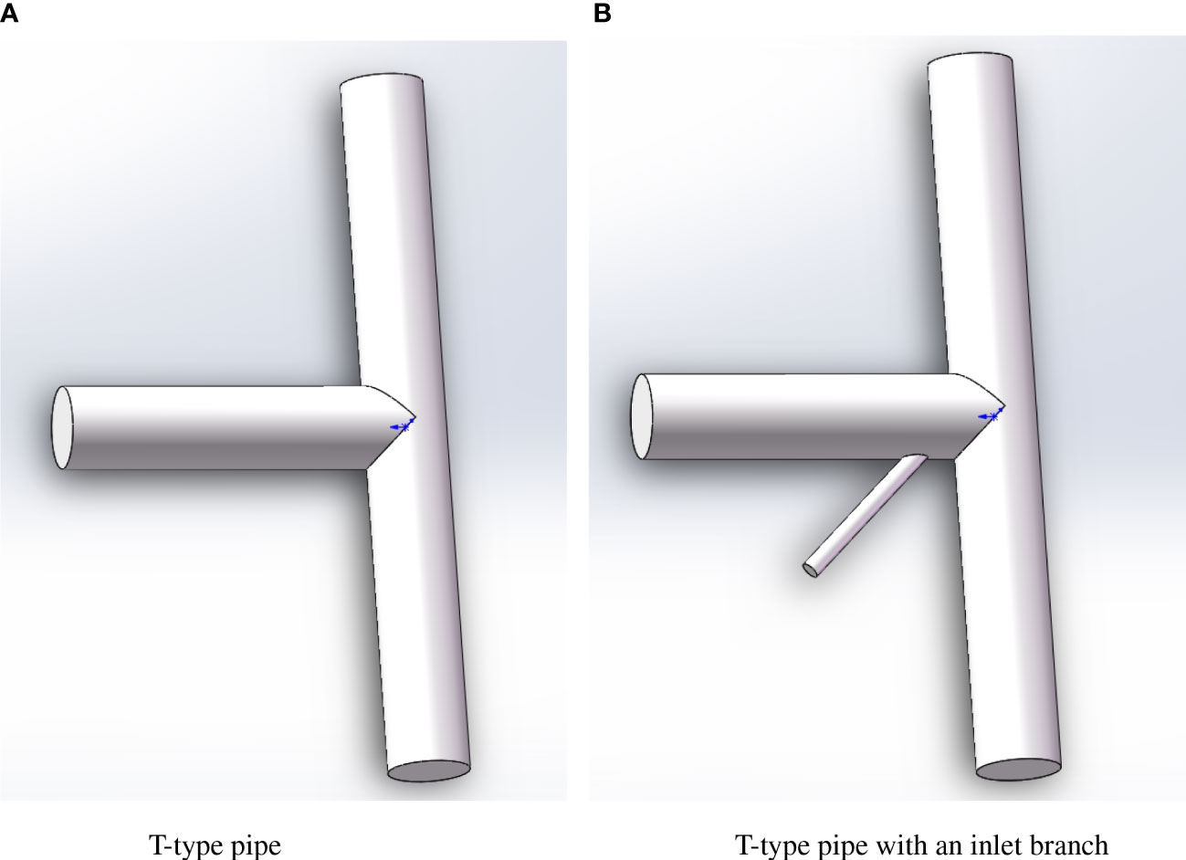
Figure 1 T-type pipes without and with a branch pipe for flow control. (A) T-type pipe. (B) T-type pipe with an inlet branch.

Water flows from the water pump to the main inlet pipe with a given flow rate and is then diverted into the two outlet pipes to two farming tanks with oxygen. Water also flows from the inlet branch and joins in the main inlet pipe to control the flow rate of the two outlet pipes. To simplify the simulations, the thickness and roughness of the pipe walls are neglected. It is also assumed that the oxygen level of seawater can be proportional to the amplitude of flow rate.

3.2 Computational domain and boundary conditions

The computational domain of T-type pipes without and with a branch inlet for flow control is shown in Figure 2. A coordinate system was established in which the origin was located at the center of the lower outlet. Q₁, Q₂, Q₃, and Q represent the flow rate at the main inlet, the upper outlet, the lower outlet, and the branch inlet, respectively. For the boundary conditions, the no-slip wall boundary condition was imposed on the pipe wall. Mass flow inlet and pressure outlet boundary conditions were employed for the inlet and outlet boundaries, respectively. A reference pressure equivalent to one standard atmospheric pressure was exerted on the upper outlet.

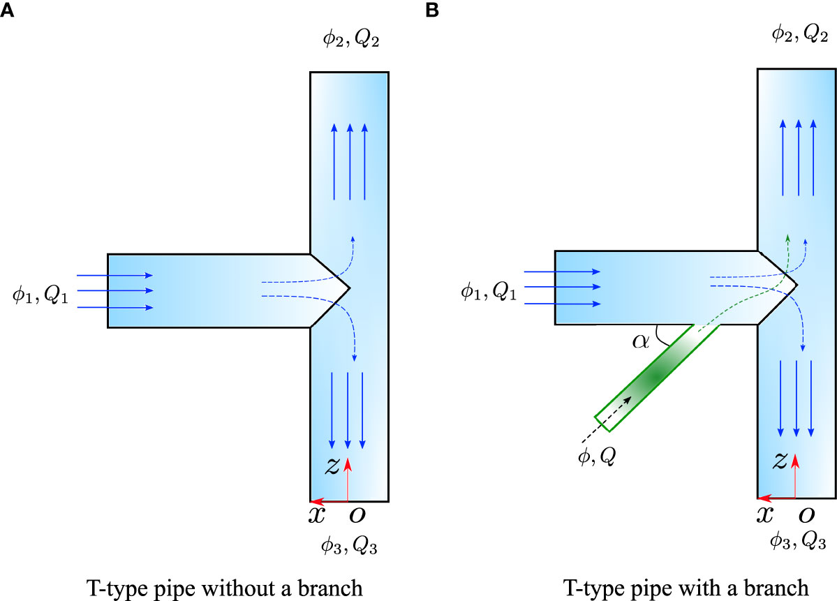
Figure 2 Computational domain of T-type pipes for flow control (A) T-type pipe without a branch (B) T-type pipe with a branch pipe.

3.3 Grid generation

In this paper, a polyhedral meshing model, which utilizes an arbitrary polyhedral cell shape to generate the core mesh with complicated geometries, was taken advantage of in the STAR-CCM+ solver. As an example, the details of grid generation for the T-type pipe with a branch inlet are shown in Figure 3. Five layers of boundary layer mesh were built to deal with the large amplitude of velocity gradient within boundary layers near the wall. The grid growth ratio was 1.5 and the non-dimensional size of the first grid height near the wall, y⁺, can be unified for the internal flows.

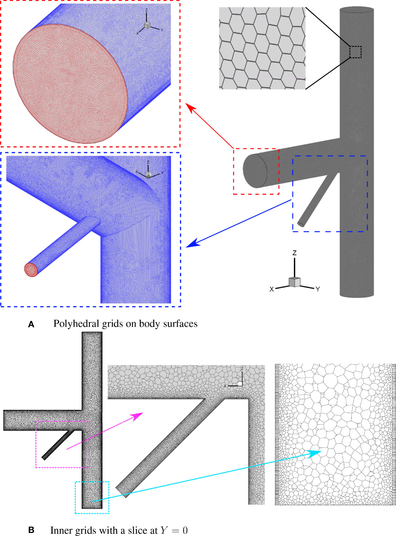
Figure 3 Grid generation for the T-type pipe with a branch (A) Polyhedral grids on body surfaces (B) Inner grids with a slice at Y = 0.

As shown in Figure 3A, the red part represents the polyhedral grids on the inlet and outlet surfaces while the blue part stands for the polyhedral grids on the wall surfaces of the T-type pipe. The grids near the connection between the main inlet pipe and the branch inlet pipe are also smoothed to improve the grid quality and numerical stability. Figure 3B presents the sliced section at the center of Y = 0 and its inner grids of the pipes. The boundary layer mesh can be observed and the inner grids are smoothed adjacent to the wall. Since the diameter of the branch inlet was relatively small, a fine base size was required to solve the flow fields accurately. Finally, the total number of grids in this paper ranges from 278,094 to 4,555,934.

3.4 Case matrix

A case matrix with various geometries, physical models, and detailed operating conditions is summarized below and presented in Table 1. Note that “TBD” is short for “to be determined”, which can be determined by the present simulations.

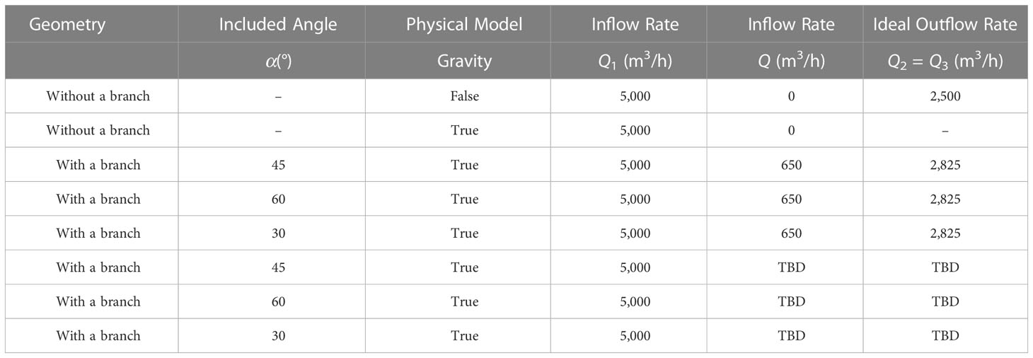
Table 1 Case matrix for 3-D simulations of water flows inside T-type pipes.

In the following studies, simulations on flow rate distributions for the T-type pipe without a branch were firstly carried out. Since the diameters of the main inlet and two outlets are the same, the ideal outflow rate for the outlet can be determined as Q₂ = Q₃ = Q_1/2 based on the conservation of mass. Firstly, the gravitational acceleration was not considered. The numerical methods were verified based on convergence studies. In this case, the result of Q₂ = Q₃ should be satisfied for the numerical simulations. The effect of the gravitational acceleration was then studied by comparing the results of the first two cases listed in Table 1. In this case, Q₂ ≠ Q₃ would be obtained for the numerical results, while the condition Q1 = Q₂ + Q₃ should always be satisfied.

Thereafter, simulations on flow rate distributions for the T-type pipe with a branch were comprehensively investigated. A given inflow rate for the branch inlet with Q = 650 (m³/h) was imposed for the branch with various included angles from 30°C to 60°C. The effect of the branch inlet was addressed. Afterwards, a couple of inflow rates for the branch inlet was tested numerically to understand how the outflow rates in two outlets can be balanced. Note that the ideal outflow rate should be Q₂ = Q₃ = (Q + Q₁)/2, which is dependent on the adjustable inflow rate for the branch inlet.

It should be noted that the Reynolds number, Re, ranged from 1.5 × 10⁶ (branch inlet) to 2.5 × 10⁶ (main inlet).

4 Numerical results and discussions

4.1 Verification for a T-type pipe

Convergence studies with various grid sizes and time steps are provided in Table 2. A total of seven cases were carried out, including five grid sizes and three time steps. The physical model, gravity, was not activated for these simulations.

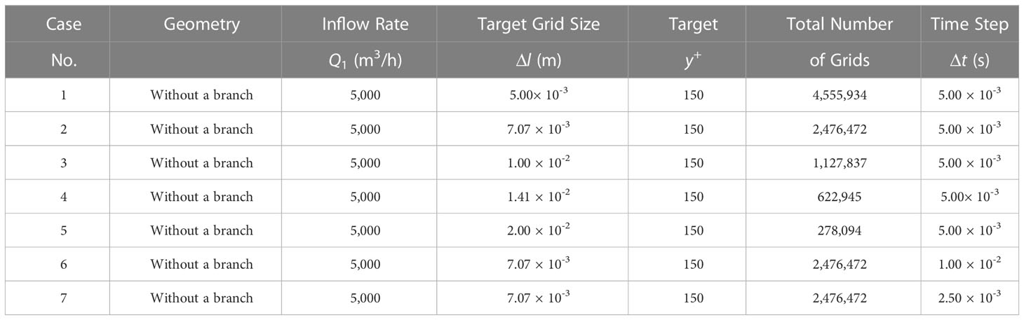
Table 2 Convergence studies of flow rates using T-type pipe without a branch.

For spatial convergence, five cases with different grid sizes in terms of Δl = 5.00 × 10^-3 to 2.00 × 10^-2 m were firstly investigated. Note that for these cases, the time step was kept the same. The convergence of the outflow rates at the upper outlet and lower outlet to Δl is shown in Figures 4A, B. It can be seen that the time histories of Q₂ and Q₃ converged to a constant value with the simulation time increased for all the cases. The final result was obtained by using the average of the results in the range of the last 500 steps. Finally, the converged results of spatial convergence are shown in Figure 5A. It can be seen that numerical results converged with the increase of the total number of grids. To save the computational resources, in the following studies, Δl = 7.07 × 10^-3 m was applied instead of the setting with the finest grids. In comparison to the analytical value of the ideal outflow rate, the discrepancies between the present numerical results and the analytical value were smaller than 1%.

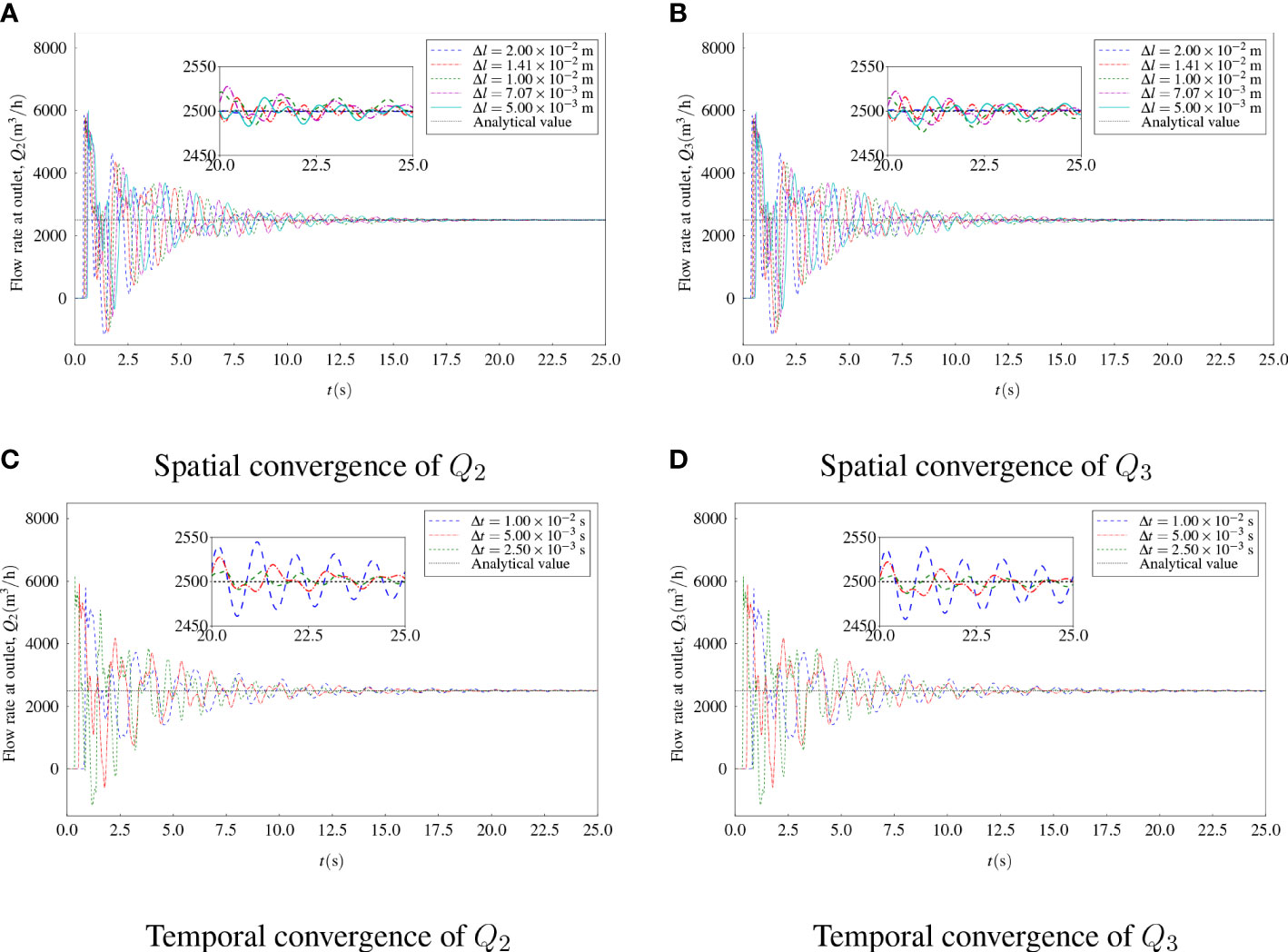
Figure 4 Convergence studies of flow rates on grid size (A) Spatial convergence of Q2 (B) Spatial convergence of Q3 (C) Temporal convergence of Q2 (D) Temporal convergence of Q3.

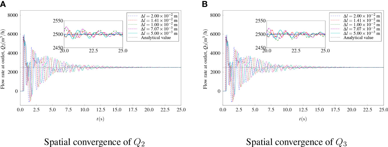
Figure 5 Results of convergence studies of flow rates (A) Results of spatial convergence (B) Results of temporal convergence.

Furthermore, a temporal convergence study was carried out using three time steps. The convergence of the outflow rates at the upper outlet and lower outlet to Δt is presented in Figures 4C, D. Oscillations of the outflow rate were observed if the time step was large. It was found that the time histories converged with the increase of the simulation time. The converged results of temporal convergence are shown in Figure 5B, which are insensitive to the change in time step for implicit simulations. In the following studies, Δt = 5 × 10^-3 s was adopted.

Therefore, a good accuracy was obtained and the numerical simulations were verified based on the convergence studies. The best-practice settings were obtained with a target grid size Δl = 7.07 × 10^-3 m and a time step Δt = 5 × 10^-3 s. The total number of grids was then 2,476,472 for the case of the T-type pipe without a branch inlet. The same settings can be applied for simulations of the T-type pipe with a branch inlet.

4.2 Effect of gravity

In this section, the influence of gravitational acceleration on the flow rate distribution of the two outflows in the T-type pipe without a branch is presented. Qualitatively, the flow rate at the upper outlet would be reduced and that at the lower outlet would be increased due to the effect of gravity. Despite the physical model, the geometry, grids, and operating conditions were kept the same for the cases without and with gravity.

Time histories of the outflow rates Q₂ and Q₃ are compared in Figure 6A and the final converged results are presented in Figure 6B. It can be seen that the convergence speed was higher and the fluctuation of the flow rates was smaller for the case with gravity. Finally, the flow rates Q₂ = 2,340.59m^3/h and Q₃ 2,659.40m³/h were obtained for the case with gravity. The result for Q₁= Q₂ + Q₃ was also obtained with a high accuracy. Therefore, the effect of gravity led to a certain flow rate deduction for the upper outlet and a flow rate increment for the lower outlet. The difference in flow rate between the upper outlet and the lower outlet could be up to 320 m³/h, equivalent to 12.8% of the ideal outflow rate.

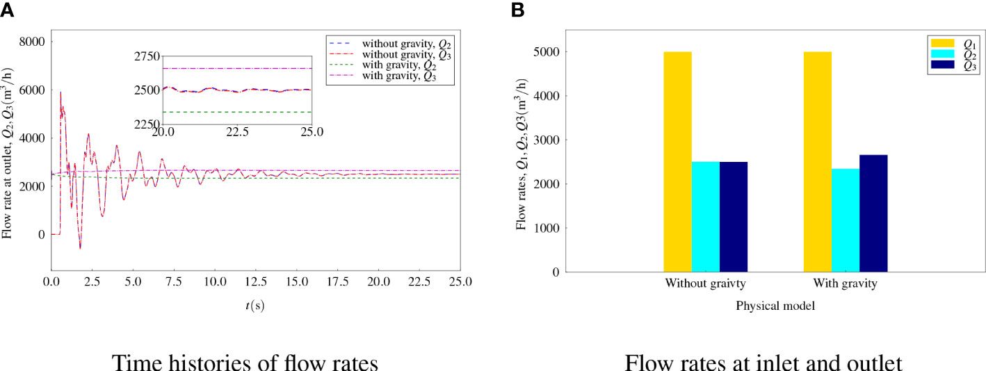
Figure 6 Flow rates for flows without and with gravity (A) Time histories of flow rates (B) Flow rates at inlet and outlet.

The flow patterns for the T-type pipe without and with gravity were obtained by the present simulations. Figure 7 presents the contours of velocity field for the central section of the T-type. In addition, the velocity distributions on the upper and lower outlet surfaces are also compared. For the physical model without gravitational accelerations, the flow pattern indicates a good symmetrical feature for the upper segment and the lower segment of the pipe. The contours of velocity for the upper outlet and the lower outlet are basically the same. It can be seen that the flow velocity in the lower segment is higher than that in the upper segment because of the effect of gravity. Moreover, the velocity contour shows non-symmetry for the result on the upper outlet and that on the lower outlet.

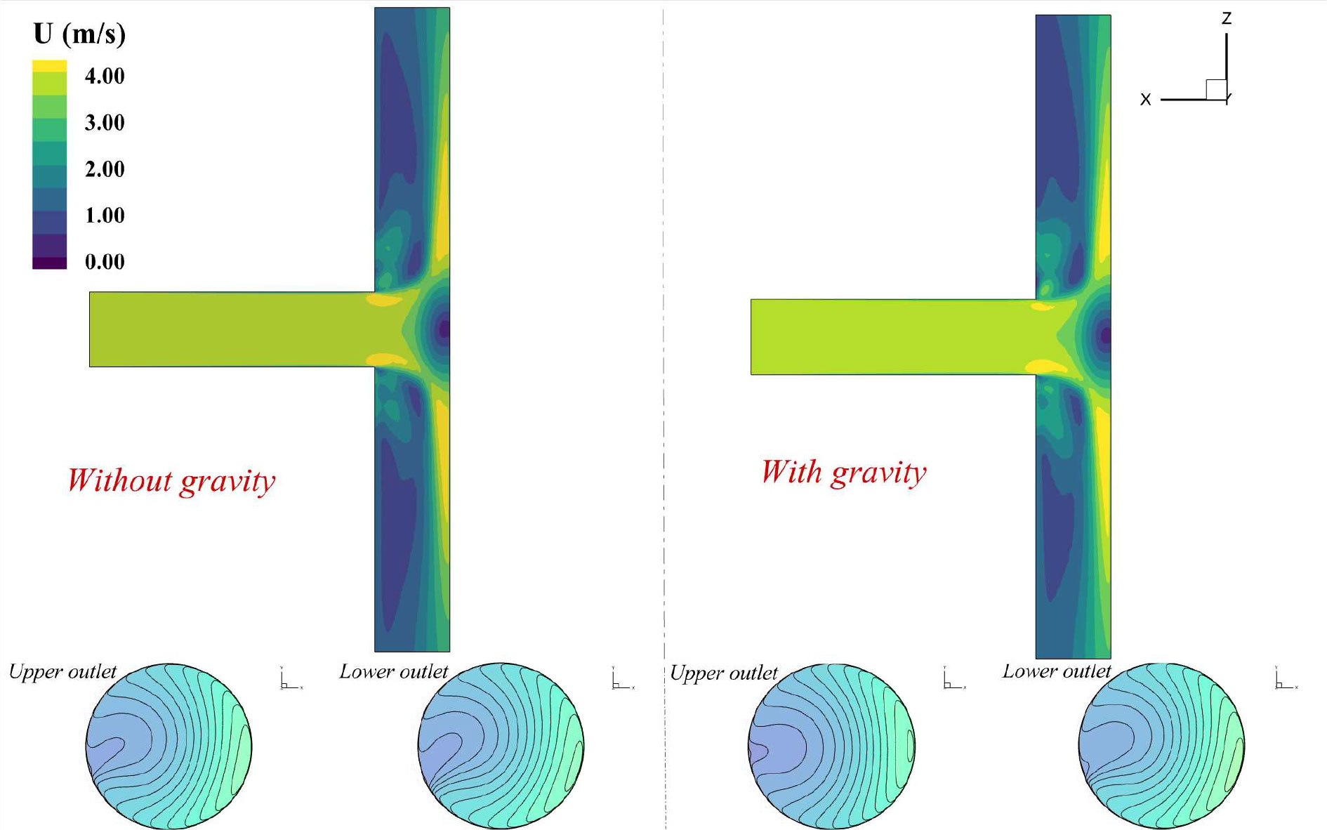
Figure 7 Contours of velocity field for flows without and with gravity.

The pressure contours for the central section of the T-type without and with gravity are shown in Figure 8. Two zones of low pressure can be observed near the perpendicular corners. A range of high pressure represented by red color was found due to the flow affecting the pipe wall. The influence of gravitational acceleration on pressure contours for the central section of the T-type was concluded as trivial.

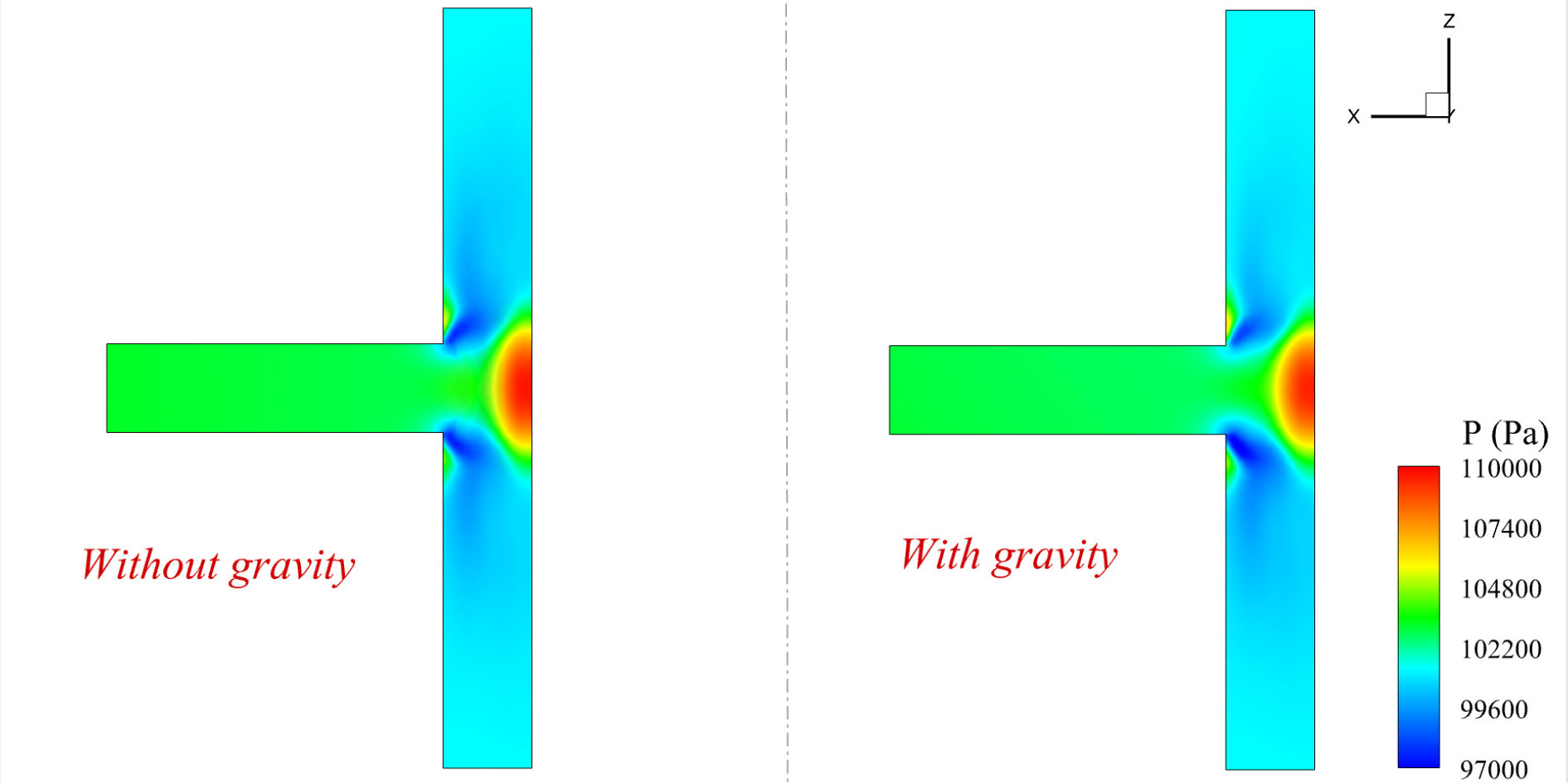
Figure 8 Contours of pressure field for flows without and with gravity.

To clearly show the detailed flow pattern inside the T-type pipe, a Line Integral Convolution (LIC) technology (Cabral and Leedom, 1993) was adopted. Based on the surface LIC algorithm, vectors defined on an arbitrary surface can be projected onto the surface and then from physical space into screen space where an image of LIC is computed. The LIC texture using velocity vectors with vorticity contours for the central section of the T-type is shown in Figure 9. Higher vorticity can be found near the corner at the connection of the inlet pipe and the outlet pipes. The influence of gravity on the flow field reduced the magnitude of vorticity near the upper corner.

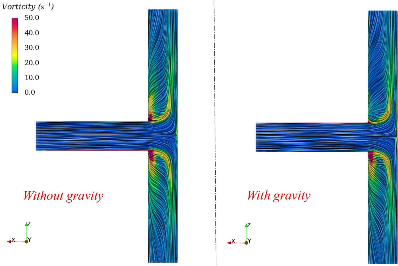
Figure 9 Contours of vorticity field with LIC for flows without and with gravity.

In addition, the three-dimensional streamlines are extracted and presented in Figure 10. The flow fields are contoured by pressures. The streamlines started from the inlet, and laminar flow was found in the inlet segment of the T-type pipe. After the flow affecting the vertical wall surface, the streamlines began to rotate and twist and vortices were generated. With the limitation of the pipe wall, the water flow rotated along the Zz-axis and flushed out at the upper and lower outlet. It can also be observed that the streamlines differed a little for the two cases without and with gravity.

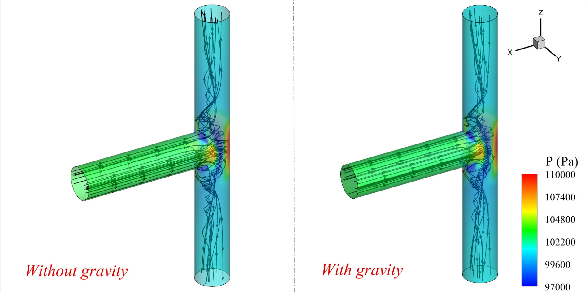
Figure 10 3-D streamlines for flows without and with gravity.

4.3 T-type pipe with a branch

The branch inlet was designed to control the flow rate inside the T-type pipe. Employing the best-practice settings, more studies were carried out to study the flow rates in the T-type pipe with a branch inlet. Two parameters were investigated for flow control, including the flow rate at the branch inlet and the included angle between the branch inlet pipe and the main inlet pipe.

The outflow rates Q₂ and Q₃ for the case without and with a branch inlet were compared. In this case, the included angle was fixed as α = 45°. The flow rate at the main inlet pipe, Q₁, was fixed as 5,000 m^3/h. It was assumed that Q = 500m³/h for flow rate at the branch inlet as an example, and time histories of flow rates at the upper and lower outlets and the final converged values are presented in Figures 11A, B, respectively. It can be concluded that the joint of the branch inlet flow leads to an increase in flow rates at both the upper and lower outlets. A new condition, i.e., $Q_1^{"}=Q+Q_1=Q_2+Q_3$, has been satisfied. However, it is not enough to address the right flow rate at the branch inlet to balance the result of Q₂ and Q₃. Therefore, an interpolation process was carried out to determine the TBD value of Q. Six more cases were studied and the flow rate at the branch inlet Q ranged from 635 to 650 m³/h. As shown in Figure 12, with the increase in flow rate at the branch inlet, the flow rate at the upper outlet tends to increase and that at the lower outlet tends to decrease. The intersection point crossing the curve of the ideal flow rate at each outlet should be the balance point. By using linear interpolation, the intersection point can be found as Q = 641.42m³/h. Therefore, the flow rate Q₂ = 2,820.42m³/h and Q_{3 =} 2,821.00m³/h were obtained, which can be regarded as Q₂ ≈ Q₃ within the error margin, and the ideal outflow rate was Q_t = 2820.71 m³/h.

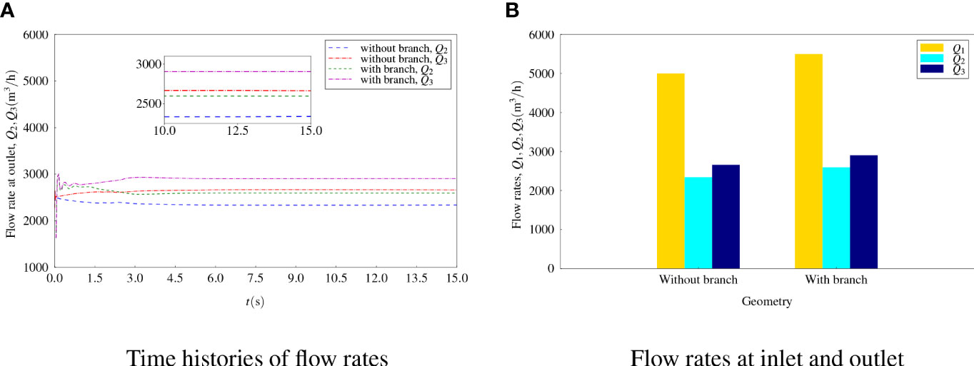
Figure 11 Flow rates for flows without and with a branch with a fixed angle (A) Time histories of flow rates. (B) Flow rates at inlet and outlet

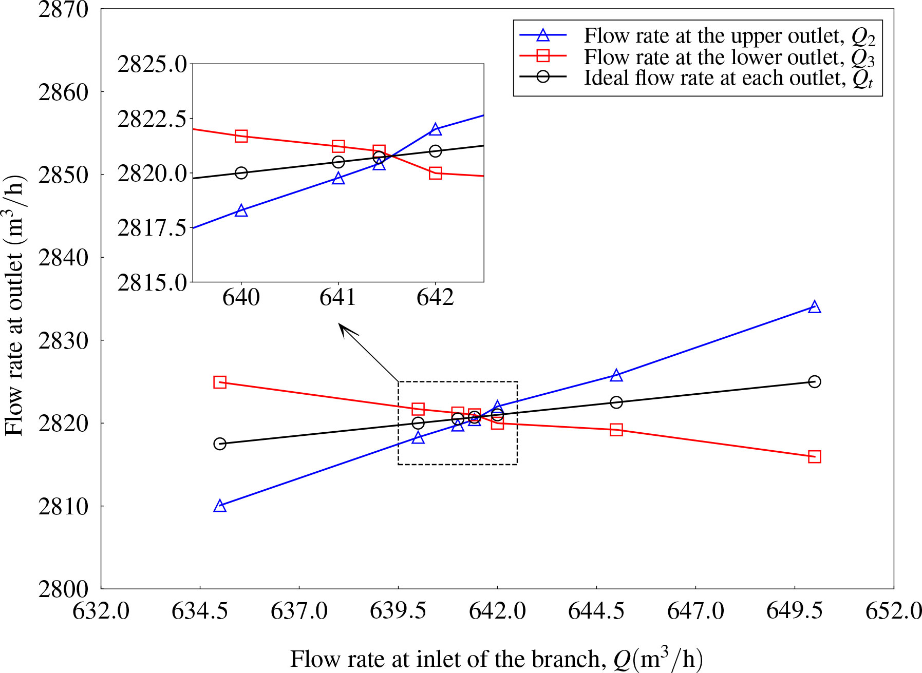
Figure 12 Flow rate at outlet with various flow rates at inlet of the branch (α = 45°).

In the following studies, a change of the included angle of the branch inlet pipe, α, was applied to propose a flow control scheme to balance the outflow rates at the upper and lower outlet. Preliminary studies have been carried out for three included angles, i.e., α = 30°, 45°, and 60°. The same branch inlet flow rate Q = 650m³/h was firstly applied to these cases to address the effect of the included angle of the branch inlet pipe. As shown in Figure 13A, time histories of the outflow rates at the upper and lower outlet converged along with the increase of simulation time. The final converged results as shown in Figure 13B were different for Q₂ and Q₃. Q₂< Q₃ was observed for the results of α = 30°. With the increase of the included angle, the flow rate Q₂ increased but the flow rate Q₃ decreased, while the flow rate of the branch inlet was fixed. For the included angle α = 45°, Q₂ > Q₃. If the angle reached 60°C, the difference between Q₂ and Q₃ was quite large.

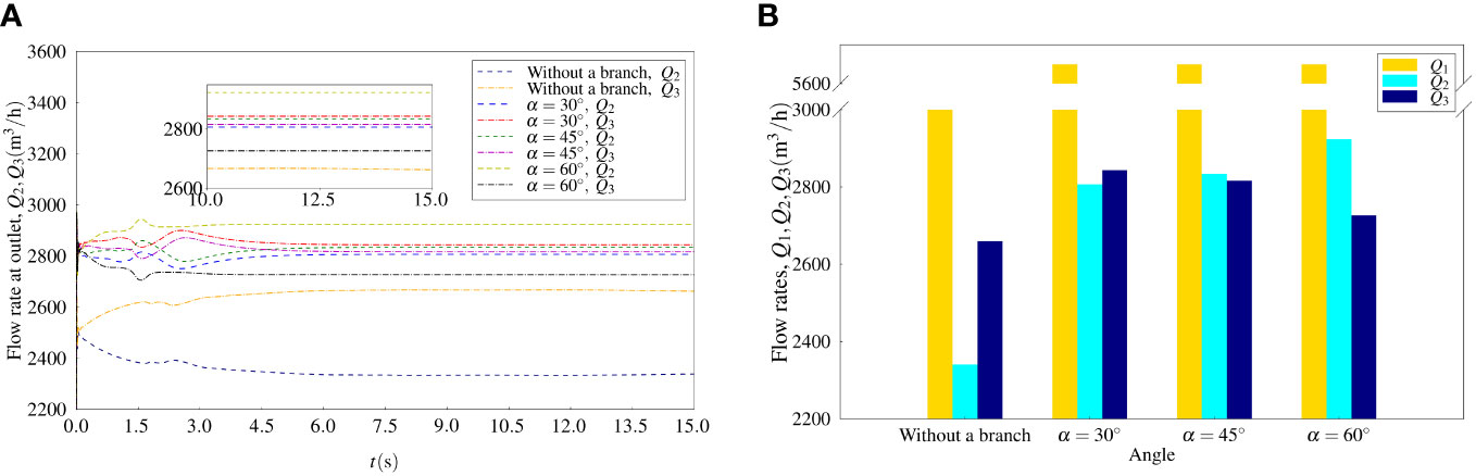
Figure 13 Flow rates for flows without and with a branch with various angles (A) Time histories of flow rates (B) Flow rates at inlet and outlet.

Similarly, interpolations were carried out to find out the balance point for the flow rate at the branch inlet with various included angles. The results for the case with α = 30° and α = 60° are shown in Figures 14, 15, respectively. For example, the error between Q₂ = 2835.06 m³/h and Q₃ = 2835.16 m³/h was less than 0.1\% (the ideal flow rate is 2835.11 m³/h at the outlet as shown in Figure 14. It can be regarded as a balance flow rate at upper and lower outlets was obtained when the flow rate at the branch inlet was Q = 670.21m³/h. Finally, the intersection points can be found as Q = 670.21m³/h and Q = 505.98m³/h for the case with α = 30° and α = 60°, respectively.

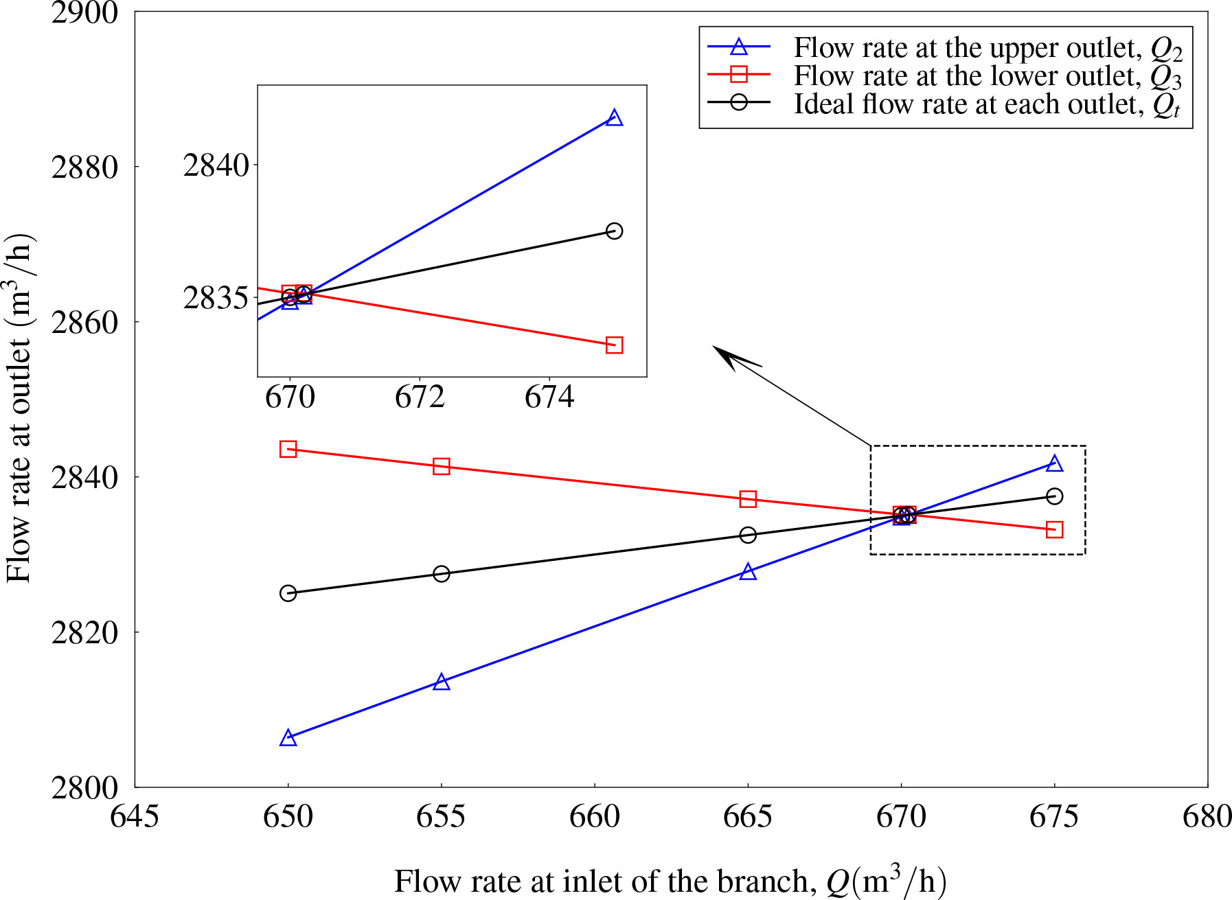
Figure 14 Flow rate at outlet with various flow rates at inlet of the branch (α = 30°).

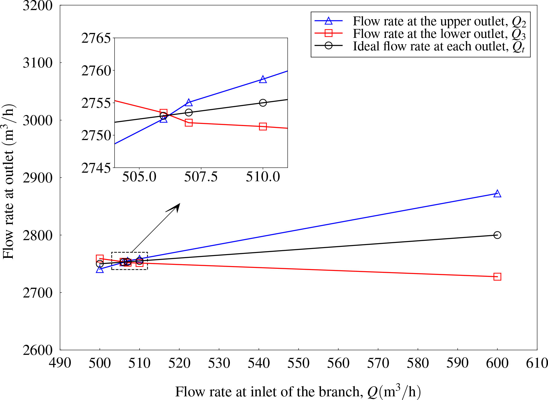
Figure 15 Flow rate at outlet with various flow rates at inlet of the branch (α = 60°).

Detailed flow fields for the T-type pipe with three included angles of the branch inlet pipe were analyzed by the present simulations. Note that the inflow rate at the balance point was presented. The contours of velocity field for the central section of the T-type and for the upper and lower outlet surfaces are shown and compared in Figure 16. For all the three cases, a high-speed inflow from the branch was obtained since the diameter of the branch inlet was much smaller than the diameter of the main inlet pipe. The high-speed inflow entering the main stream was then decelerated and the water flows in the outlet segment pipe became more turbulent. The velocity contours for the upper outlet and the lower outlet were changed due to the introduction of the branch inflow. In terms of the geometry of the branch, it can be seen that the flow velocity was quite asymmetrical for contours on the upper outlet and the lower outlet, especially for the case with an included angle α = 60°.

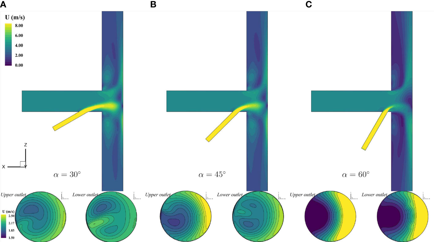
Figure 16 Contours of velocity field for flows with various angles (A) α = 30° (B) α = 45° (C) α = 60°.

The pressure contours for the central section of the T-type with various included angles are shown in Figure 17. Two zones of low pressure can be observed near the perpendicular corners. The smaller the included angle was, the fewer changes in pressure distribution can be observed. For a large included angle, e.g., α = 60, the zone of low pressure was expanded and the original shape of high pressure was affected.

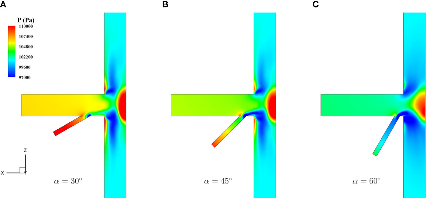
Figure 17 Contours of pressure field for flows with various angles (A) α = 30° (B) α = 45° (C) α = 60°.

The LIC texture using velocity vectors with vorticity contours for the T-type with various included angles is shown in Figure 18. Vortices can be found near the corner at the connection of the inlet pipe and the outlet pipes, and the corner near the branch inlet pipe. The three-dimensional streamlines are extracted and presented in Figure 19, as well as the pressure contours. The streamlines rotated much more violently for the case with a large included angle like α = 60°. Compared with that of the flow in the upper segment pipe, the vorticity of the flow in the lower segment pipe was higher due to the effect of the branch inlet pipe.

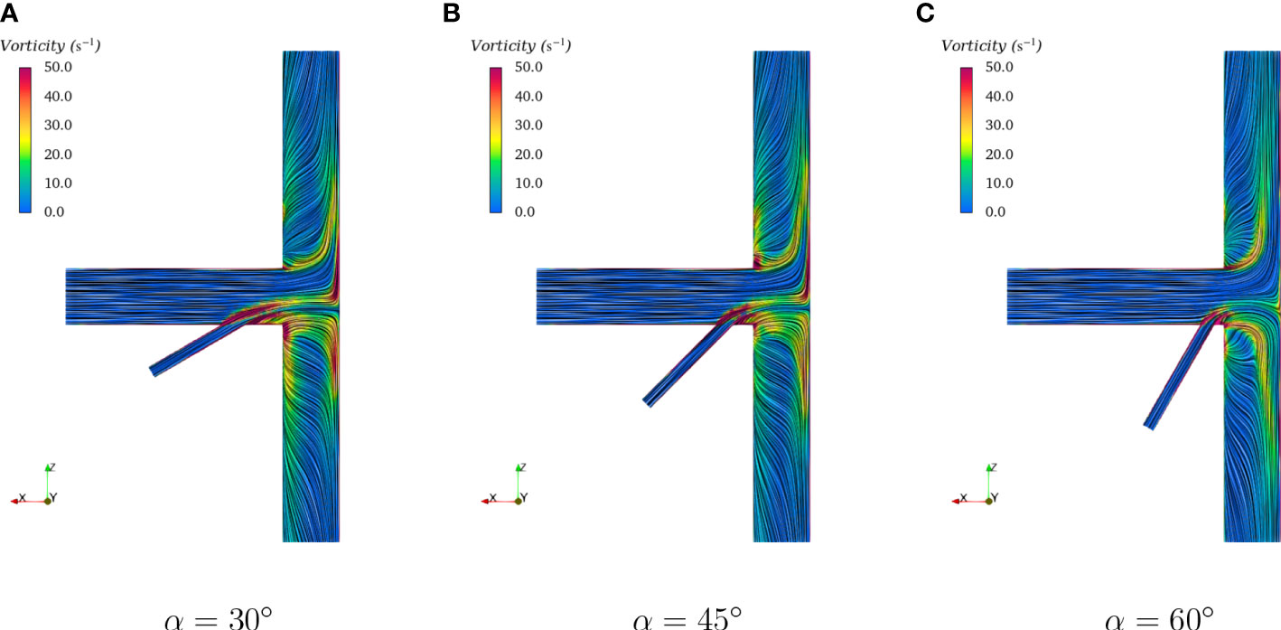
Figure 18 Contours of vorticity field with LIC for flows with various angles (A) α = 30° (B) α = 45° (C) α = 60°.

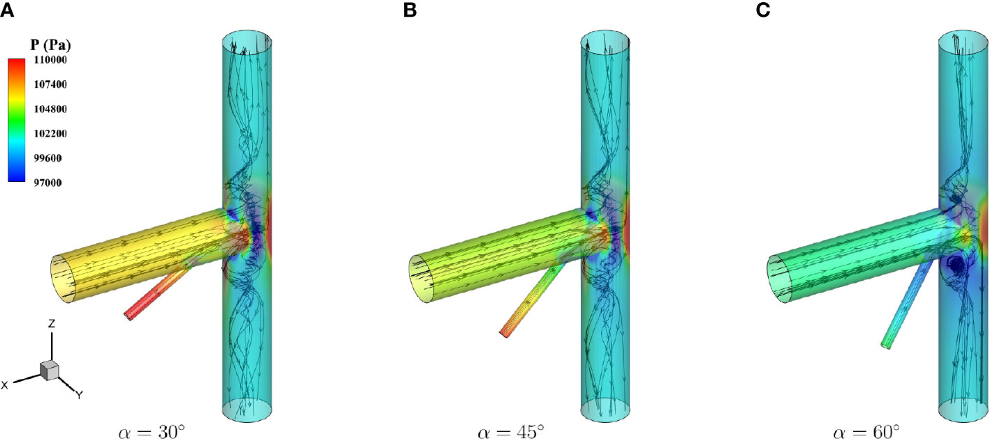
Figure 19 3-D streamlines for flows with various angles (A) α = 30° (B) α = 45° (C) α = 60°.

5 Conclusions

In this paper, we studied the flow rates in a flow diverter, i.e., a T-type pipe, and its flow control using a special branch for water pumping systems in the cruising aquaculture vessel, Guoxin 1. To obtain a balanced oxygen supply for two farming tanks, a balanced water flow rate should be guaranteed if one pump is available. The flow rate at the outlet can be influenced by several factors, e.g., the gravitational acceleration, the flow rate at the branch inlet, and the included angle between the branch inlet pipe and the main inlet pipe. Equilibrium outflow rates were desired to efficiently supply the oxygen to different aquaculture tanks. The following conclusions can be drawn based on the numerical results in this work. The research of this paper can provide a reference for the oxygen supply between aquaculture tanks to maintain a healthy culturing environment.

1. Gravity would affect the unbalanced flow rate due to the altitude difference in multiple farm tanks, especially in cruising aquaculture vessels. According to the present three-dimensional simulations, the difference in flow rate at the upper and lower outlet could be as large as 12.8%.

2. It is reasonable for the flow control in the tee pipe to adopt a branch inlet with a small diameter and a high-speed water inflow. A balance point can be interpolated by adjusting the flow rate at the branch inlet to obtain equilibrium outflow rates in two outlets.

3. The branch inlet for flow control should be equipped with a reasonable included angle with the main inlet pipe. A high inflow rate at the branch inlet is required if the included angle was small. However, the advantage of a small included angle is the low impact of the additional flow on the flow patterns. It can be concluded that a low-speed inflow rate at the branch inlet for the branch with a large included angle is necessary while the flow field is significantly affected by the additional inlet flow.

Data availability statement

The raw data supporting the conclusions of this article will be made available by the authors, without undue reservation.

Author contributions

WH: Conceptualization, writing, reviewing, editing, and data analysis. RZ: Numerical simulations, supervision, writing, reviewing, and editing. All authors contributed to the article and approved the submitted version.

Funding

This work was financially supported by the National Key Research and Development Program of China (Grant No.2022YFD2401101), the Program of Qingdao National Laboratory for Marine Science and Technology (Grant No.2022QNLM030001-3), and the National Natural Science Foundation of China (Grant No. 52201394).

Conflict of interest

The authors declare that the research was conducted in the absence of any commercial or financial relationships that could be construed as a potential conflict of interest.

Publisher’s note

All claims expressed in this article are solely those of the authors and do not necessarily represent those of their affiliated organizations, or those of the publisher, the editors and the reviewers. Any product that may be evaluated in this article, or claim that may be made by its manufacturer, is not guaranteed or endorsed by the publisher.

References

Aryawan W., Putranto T. (2018). The hydrodynamics performance of aquaculture fishing vessel in variation of deadrise angle and sponson. Int. J. Mechanical Production 8, 263–272. doi: 10.24247/ijmperdapr201829
Cabral B., Leedom L. C. (1993). “Imaging vector fields using line integral convolution,” in Proceedings of the 20th annual conference on Computer graphics and interactive techniques. 263–270. Association for Computing Machinery Anaheim, CA, United States
Chen Y., Huang W., Shan X., Chen J., Weng H., Yang T., et al. (2020). Growth characteristics of cage-cultured large yellow croaker larimichthys crocea. Aquac. Rep. 16, 100242. doi: 10.1016/j.aqrep.2019.100242
Costa N., Maia R., Proenca M., Pinho F. (2006). Edge effects on the flow characteristics in a 90 deg tee junction. 128(6), 1204–1217 doi: 10.1115/1.2354524
Duarte S., Reig L., Masaló I., Blanco M., Oca J. (2011). Influence of tank geometry and flow pattern in fish distribution. Aquac. Eng. 44, 48–54. doi: 10.1016/j.aquaeng.2010.12.002
Editorial Staff (2022) China Delivers guoxin 1, world’s first tanker-sized aquaculture vessel that will produce more than 3,700 tons per year. Available at: https://aquaculturemag.com/2022/06/10/china-delivers-guoxin-1-worlds-first-tanker-sized-aquaculture-vessel-that-will-produce-more-than-3700-tons-per-year/.
Edwards K., Finn D. (2015). Generalised water flow rate control strategy for optimal part load operation of ground source heat pump systems. Appl. Energy 150, 50–60. doi: 10.1016/j.apenergy.2015.03.134
Guo X., Li Z., Cui M., Wang B. (2020). Numerical investigation on flow characteristics of water in the fish tank on a force-rolling aquaculture platform. Ocean Eng. 217, 107936. doi: 10.1016/j.oceaneng.2020.107936
Han F., Ong M. C., Xing Y., Li W. (2020). Three-dimensional numerical investigation of laminar flow in blind-tee pipes. Ocean Eng. 217, 107962. doi: 10.1016/j.oceaneng.2020.107962
He Y. (2008). The euler implicit/explicit scheme for the 2d time-dependent navier-stokes equations with smooth or non-smooth initial data. Mathematics Comput. 77, 2097–2124. doi: 10.1090/S0025-5718-08-02127-3
Hvas M., Folkedal O., Oppedal F. (2021). Fish welfare in offshore salmon aquaculture. Rev. Aquac. 13, 836–852. doi: 10.1111/raq.12501
Kassem T., Shahrour I., El Khattabi J., Raslan A. (2021). Smart and sustainable aquaculture farms. Sustainability 13, 10685. doi: 10.3390/su131910685
Lai Y., So R., Anwer M., Hwang B. (1991). “Calculations of a curved-pipe flow using reynolds stress closure,” in Proceedings of the Institution of Mechanical Engineers, Part C: Mechanical Engineering Science, Vol. 205. 231–244. SAGE Publications Sage UK: London, England
Launder B. E., Spalding D. B. (1983). “The numerical computation of turbulent flows,” in Numerical prediction of flow, heat transfer, turbulence and combustion (Elsevier), 96–116. Numerical Prediction of Flow. Heat Transfer, Turbulence and Combustion, 3
Lekang O.-I. (2020). Aquaculture engineering (John Wiley & Sons) Norwegian University of Life Science, Blackwell Publishing.
Li Z., Guo X., Cui M. (2022). Numerical investigation of flow characteristics in a rearing tank aboard an aquaculture vessel. Aquac. Eng. 98, 102272. doi: 10.1016/j.aquaeng.2022.102272
Li G., Pan L., Hua Q., Sun L., Lee K. Y. (2019). Water pump control: A hybrid data-driven and model-assisted active disturbance rejection approach. Water 11, 1066. doi: 10.3390/w11051066
Ma C., Zhao Y.-P., Bi C.-W. (2022). Numerical study on hydrodynamic responses of a single-point moored vessel-shaped floating aquaculture platform in waves. Aquac. Eng. 96, 102216. doi: 10.1016/j.aquaeng.2021.102216
Mansi F., Cannone E. S. S., Caputi A., De Maria L., Lella L., Cavone D., et al. (2019). Occupational exposure on board fishing vessels: Risk assessments of biomechanical overload, noise and vibrations among worker on fishing vessels in southern italy. Environments 6, 127. doi: 10.3390/environments6120127
Masaló I., Oca J. (2014). Hydrodynamics in a multivortex aquaculture tank: effect of baffles and water inlet characteristics. Aquac. Eng. 58, 69–76. doi: 10.1016/j.aquaeng.2013.11.001
Menter F. R. (1994). Two-equation eddy-viscosity turbulence models for engineering applications. AIAA J. 32, 1598–1605. doi: 10.2514/3.12149
Mockett C., Fuchs M., Thiele F. (2012). Progress in des for wall-modelled les of complex internal flows. Comput. Fluids 65, 44–55. doi: 10.1016/j.compfluid.2012.03.014
Moukalled F., Mangani L., Darwish M. (2016). “The finite volume method,” in The finite volume method in computational fluid dynamics (Springer), 103–135. Springer International Publishing
Oca J., Masaló I. (2007). Design criteria for rotating flow cells in rectangular aquaculture tanks. Aquac. Eng. 36, 36–44. doi: 10.1016/j.aquaeng.2006.06.001
Oca J., Masalo I. (2013). Flow pattern in aquaculture circular tanks: Influence of flow rate, water depth, and water inlet & outlet features. Aquac. Eng. 52, 65–72. doi: 10.1016/j.aquaeng.2012.09.002
Oca J., Masaló I., Reig L. (2004). Comparative analysis of flow patterns in aquaculture rectangular tanks with different water inlet characteristics. Aquac. Eng. 31, 221–236. doi: 10.1016/j.aquaeng.2004.04.002
Padala A., Zilber S. (1991). “Expert systems and their use in aquaculture,” in Rotifer and microalgae culture systems. proceedings of a US-Asia workshop, 221–227. Honolulu, HI the publisher is the Oceanic Institute.
Romli M. A., Daud S., Raof R. A. A., Ahmad Z. A., Mahrom N. (2018). Aquaponic growbed water level control using fog architecture. J. Physics: Conf. Ser. 1018, 012014. doi: 10.1088/1742-6596/1018/1/012014
Shih T.-H., Liou W. W., Shabbir A., Yang Z., Zhu J. (1994). A new k-epsilon eddy viscosity model for high reynolds number turbulent flows. Computers & Fluids. (Elsevier) 24(3), 227–238 doi: 10.1016/0045-7930(94)00032-T
Spalart P., Allmaras S. (1992). “A one-equation turbulence model for aerodynamic flows,” in 30th aerospace sciences meeting and exhibit. 439. American Institute of Aeronautics and Astronautics Reno, NV, U.S.A.
Tello M., e Silva S. R., Soares C. G. (2011). Seakeeping performance of fishing vessels in irregular waves. Ocean Eng. 38, 763–773. doi: 10.1016/j.oceaneng.2010.12.020
The Fish Site (2020) Chinese Start construction of 200,000-tonne mobile fish farm. Available at: https://thefishsite.com/articles/chinese-start-construction-of-first-200-000-tonne-mobile-fish-farm.
Ullah I., Kim D. (2018). An optimization scheme for water pump control in smart fish farm with efficient energy consumption. Processes 6, 65. doi: 10.3390/pr6060065
Urrea C., Páez F. (2021). Design and comparison of strategies for level control in a nonlinear tank. Processes 9, 735. doi: 10.3390/pr9050735
Venkatakrishnan V. (1995). Convergence to steady state solutions of the euler equations on unstructured grids with limiters. J. Comput. Phys. 118, 120–130. doi: 10.1006/jcph.1995.1084
Wilcox D. C. (2008). Formulation of the kw turbulence model revisited. AIAA J. 46, 2823–2838. doi: 10.2514/1.36541
Xue B., Zhao Y., Bi C., Cheng Y., Ren X., Liu Y. (2022). Investigation of flow field and pollutant particle distribution in the aquaculture tank for fish farming based on computational fluid dynamics. Comput. Electron. Agric. 200, 107243. doi: 10.1016/j.compag.2022.107243
Zhang S.-Y., Li G., Wu H.-B., Liu X.-G., Yao Y.-H., Tao L., et al. (2011). An integrated recirculating aquaculture system (RAS) for land-based fish farming: The effects on water quality and fish production. Aquac. Eng. (Elsevier) 45 (3), 93–102. doi: 10.1016/j.aquaeng.2011.08.001
Zhao Y., Xue B., Bi C., Ren X., Liu Y. (2022). Influence mechanisms of macro-infrastructure on micro-environments in the recirculating aquaculture system and biofloc technology system. Rev. Aquac. doi: 10.1111/raq.12713
Keywords: offshore fish farming, aquaculture vessel, flow in pipes, flow control, computational fluid dynamics, internal flow
Citation: Huang W and Zha R (2023) Numerical studies on internal flow in pipelines of an aquaculture vessel and flow control using a special branch pipe. Front. Mar. Sci. 10:1140285. doi: 10.3389/fmars.2023.1140285
Received: 08 January 2023; Accepted: 20 February 2023;
Published: 10 March 2023.
Edited by:
Fukun Gui, Zhejiang Ocean University, ChinaReviewed by:
Hung-Jie Tang, National Cheng Kung University, TaiwanHaocai Huang, Zhejiang University, China
Copyright © 2023 Huang and Zha. This is an open-access article distributed under the terms of the Creative Commons Attribution License (CC BY). The use, distribution or reproduction in other forums is permitted, provided the original author(s) and the copyright owner(s) are credited and that the original publication in this journal is cited, in accordance with accepted academic practice. No use, distribution or reproduction is permitted which does not comply with these terms.
*Correspondence: Ruosi Zha, zhars@mail.sysu.edu.cn